Hydra: A Parallel Adaptive Grid Code

F.R.Pearce^,, H.M.P.Couchman

F.R.Pearce@durham.ac.uk, couchman@coho.astro.uwo.ca

Subject headings: methods: numerical – cosmology: theory – hydrodynamical simulation

Abstract

We describe the first parallel implementation of an adaptive particle-particle, particle-mesh code with smoothed particle hydrodynamics. Parallelisation of the serial code, “Hydra”, is achieved by using CRAFT, a Cray proprietary language which allows rapid implementation of a serial code on a parallel machine by allowing global addressing of distributed memory.

The collisionless variant of the code has already completed several 16.8 million particle cosmological simulations on a 128 processor Cray T3D whilst the full hydrodynamic code has completed several 4.2 million particle combined gas and dark matter runs. The efficiency of the code now allows parameter-space explorations to be performed routinely using $64^{3}$ particles of each species. A complete run including gas cooling, from high redshift to the present epoch requires approximately 10 hours on 64 processors.

In this paper we present implementation details and results of the performance and scalability of the CRAFT version of Hydra under varying degrees of particle clustering.

1 Introduction

A key goal of contemporary cosmology is to understand the growth of structure; that is to connect the spectrum of linear fluctuations which exists at the epoch of recombination (at present unknown) with the highly non-linear galaxies and clusters that we observe at present. Simulations of cosmic structure are amongst the most ambitious supercomputer applications: the huge range in observed structures, from sub-galactic to the largest superclusters and voids, perhaps a factor of $10^{9}$ in mass, presents a formidable numerical challenge.

The large range of density contrasts and complicated geometries that arise in cosmological simulations make Lagrangian particle methods popular choices for modelling the growth of structure. Typically, we wish to model a representative volume of the universe (corresponding to $\sim 0.1\%$ of the observable volume) over a period of 10 billion years. A contemporary simulation might use of order 10 million particles to represent the matter density in the universe. Initially these particles are distributed nearly uniformly within a triply periodic cube. The simulations follow the motion of these particles as they move under the influence of self gravity (and short range gas forces if appropriate). The push for ever higher resolution in such simulations has inevitably led to the use of parallel supercomputers, both because of the total processing power available but also, equally importantly, in order to satisfy the huge memory demands of these programs.

The trend towards the use of parallel supercomputers for large-scale cosmological simulations is clear, but is not without problems. We will address many of the issues confronting parallel particle codes in this paper, with emphasis on those of particular importance to particle–grid codes. In general, Lagrangian particle methods are hard to load balance. Static load balancing techniques do not work well because the distribution of particles relative to the necessary underlying Eulerian computational framework changes dynamically, and can become highly non-uniform. Further, the locations at which structures develop are not known accurately beforehand. This causes severe problems even for dynamic load balancing strategies. In this paper we outline our approach to solving these problems through the use of an adaptive grid refinement technique. This reduces the total amount of computational work and allows us to break the problem into many smaller parts which can then be efficiently distributed over the processors. We conclude this part of the introduction with a brief overview of the development of N-body particle techniques. More details can be found in the reviews of Sellwood (1987) and Couchman (1997).

Since the pioneering work of von Hoerner (1960) and Aarseth (1963) significant advances have been made towards numerical solution of the gravitational N-body problem. The early codes used a direct summation (here “particle-particle” or PP) approach, directly accumulating the force on each particle from the contributions of all other particles. The computing time required for this method scales as $O(N^{2})$ and for more than a few thousand particles becomes prohibitively expensive, unless application-specific hardware is used (e.g. GRAPE boards, see Steinmetz 1996).

The limit on particle number imposed by the undesirable scaling properties of PP codes has been circumvented in more recent codes by approximating the gravitational potential. All of these methods correspond in some way to a decomposition of the field due to distant particles in terms of various basis functions. Two general approaches have been popular. The method used first (and from which the method we describe in this paper is derived) was to represent the gravitational field on a mesh of fixed resolution (e.g., Miller 1978, Miller & Smith 1980). Efficient solution methods for Poisson’s equation on regular meshes, such as the FFT convolution, allow an algorithm with computation time which scales as $\sim O(N\log N)$, although the force resolution is limited to roughly two grid separations. These types of methods will be referred to here as Particle–Mesh (PM) codes.

More recently codes have been developed which represent the field via a multipole expansion. The two main variants of this approach are the various “tree codes” (Appel 1985, Jernigan 1985, Barnes & Hut 1986), and the true multipole expansion methods (van Albada & van Gorkum 1977, Villumsen 1982, Greengard & Rokhlin 1987). These methods have an advantage over grid-based codes in that their resolution is not limited by the grid scale. This is desirable in order to be able to correctly model bound objects at fixed physical separation within a simulation cube which is comoving with the universal expansion. It is possible to use a very fine mesh in order to reproduce forces over a wider range of scales but this increases both the storage requirement and computation time, as well as leading to inefficiency in regions of low particle density. An alternative method for overcoming the lack of sub-grid scale forces in conventional grid schemes is to combine these techniques with PP methods. In these hybrid codes the direct sum is performed only over nearby neighbours out to a distance necessary to augment the fixed resolution grid force to the force required overall.

Grid-based codes, in particular particle-particle, particle-mesh, (P³M) codes, have been applied to a variety of problems, ranging from the formation of large scale structure and galaxy clusters to galaxy mergers and galaxy formation (e.g., Efstathiou et al. 1985, 1988, Pearce, Thomas & Couchman 1993, 1994). Several authors (Evrard 1990, Thomas & Couchman 1992) have incorporated Smoothed Particle Hydrodynamics (SPH—Monaghan 1992) to model gas processes. P³M is very efficient in terms of memory use, but in general is very expensive when the amount of clustering becomes high and the number of neighbours in the PP sum increases. The use of adaptive refinement to increase the grid resolution in selected regions (Couchman 1991) has ameliorated this problem and the latest workstations can run simulations with $N\sim 7$ million particles in around a month (Cole & Lacey 1996).

The P³M method does not lend itself easily to parallelisation for a number of reasons. As described above, the mapping from Lagrangian particle space to the Eulerian grid can lead to load balancing problems and difficulties with data decomposition on distributed memory computers. The advantages of grid-based codes in terms of memory usage and the computational simplicity of regular grids are substantially reduced in comparison to the more general data-structure employed by “Tree” codes by these parallelization issues. Efficient parallel PM implementations have been constructed (Ferrell & Bertschinger 1994), and there are parallel PP schemes (Ferrell & Bertschinger 1995), it is difficult, however, to produce a combined method that makes efficient use of memory and has a good communication strategy. We discuss the parallelisation of a grid-based code here; the parallelisation of treecodes has been discussed elsewhere, for example, Dubinski (1996), Salmon (1991), Davé, Dubinski & Hernquist (1997).

The British supercomputing community has invested in a Cray T3D which is installed in Edinburgh. This is a massively parallel, distributed memory MIMD (multiple instruction, multiple data) machine with 512 processors. These processors are linked together in a toroidal network with high speed interconnections designed to minimise the overhead of inter-processor communication. Each node has a 150Mhz DEC Alpha EV4 processor and associated custom hardware, and has 64Mb of memory per node.

In this paper we will describe a parallel implementation of a serial P³M–SPH code, “Hydra” (Couchman, Thomas & Pearce 1995), for the T3D platform using Cray’s proprietary CRAFT software. This code (parallel Hydra) is the first parallel adaptive particle-particle, particle-mesh plus smoothed particle hydrodynamics algorithm. CRAFT has enabled us to quickly modify the serial algorithm for parallel execution.

The paper is laid as follows. In section 2 we describe the serial operation of Hydra and in section 3 deal with the problems of porting the code to parallel machines. In section 4 we look at the code’s performance on the Cray T3D, in particular the load balance and speed for both clustered and unclustered particle distributions.

2 Hydra

Hydra—an implementation of Smoothed Particle Hydrodynamics (SPH) in an adaptive P³M code (Couchman, Thomas & Pearce 1995) is the endpoint of several stages of code development which we describe below before giving a more detailed description of Hydra itself.

The fundamental drawback of the PP method, as noted above, is the rapidly increasing computational cost of the $O(N^{2})$ sum over all particle pairs, which becomes prohibitive for $N$ greater than a few thousand. The most straightforward way of circumventing this problem (borrowed initially from plasma physics) involves smoothing the particles onto a uniform grid. The potential corresponding to the sampled mass distribution is solved for using a fast Fourier transform (FFT) convolution method. The grid potential is then differenced and the forces interpolated back to the particle positions. The computational cost of the “particle-mesh” ($PM$) method scales as $\alpha N+\beta L^{3}\log L$, where $\alpha$ and $\beta$ are constants, $N$ is the number of particles and $L$ is the size of the mesh. Typically $N\sim(L/2)^{3}$, which suggests the familiar $\sim O(N\log N)$ scaling.

The main drawback of this approach is that it cannot reproduce structure on scales less than roughly 2 mesh spacings; the Nyquist wavelength of the grid. In three dimensions improving the resolution by increasing the grid size is problematic due to the rapidly increasing memory requirement: a single grid with $512^{3}$ cells requires $128\,$Mwords of memory. The advantages of FFT-based PM schemes are that they are extremely fast, the speed is independent of the degree of particle clustering and the boundaries are automatically periodic. The latter feature, a by-product of using an FFT potential solver, is a useful means of modelling a section of a very much larger, or infinite, universe.

The next advance, deriving again from plasma physics (Hockney & Eastwood 1981), was to combine the PP and PM methods to produce the hybrid “particle-particle, particle-mesh” (P³M) scheme. This method was first used in Astrophysics by Efstathiou & Eastwood (1981). This method splits the gravitational force into two components, long- and short-range. The PM method is used to solve for the long-range component and, on scales smaller than about two grid spacings the ‘soft’ mesh force is augmented by a direct PP sum over near neighbours. The calculation of the PP part proceeds by binning particles onto a coarse mesh which is then used to search efficiently for near neighbours to include in the short range component of the force calculation.

The cputime for this method scales as;

$$t_{\rm P^{3}M}\sim\alpha N+\beta L^{3}\log L+\gamma\sum_{pp^{\prime}}N_{p}N_{p^{\prime}}$$ (1)

where the first two terms come from the PM scaling from above and $\gamma$ is a constant. $N_{p}$ is the number of particles in the coarse PP mesh cell $p$; the sum over $p$ is over all cells in the mesh, whilst $p^{\prime}$ ranges over the cell $p$ and its 26 neighbour cells. If the particles are uniformly distributed throughout the computational volume and the PM mesh has been chosen such that $L^{3}\mathrel{\hbox{\hbox to0.0pt{\hbox{\lower 4.0pt\hbox{$\sim$}}\hss}\hbox{$>$}}}N$, then $N_{p}$ will be a small constant and the scheme scales roughly as $O(N\log N)$ as with the PM method. This technique produces a scheme with much better spatial resolution than the PM method and much greater speed than the PP method. The difficulty occurs when heavy clustering is present as then the number of neighbours, $\sum N_{p^{\prime}}$ is spatially variable and may become very large. Under these conditions the $O(N^{2})$ nature of the third term of equation (1) begins to dominate and the overall runtime increases rapidly.

This problem was solved by automatically placing higher resolution sections of grid within the original framework of the standard P³M scheme (Couchman 1991). In this case computational “hotspots” are identified where the work of the short-range PP calculation will be high and a finer grid is placed in this region. This reduces the range of the PP interaction and results in a corresponding decrease in $\sum N_{p^{\prime}}$. This lowers the overall computational cost despite an increase in the grid-based work of the first and second terms in equation 1 above.

Finally, smoothed particle hydrodynamics (SPH) was incorporated into the adaptive P³M code to form Hydra. SPH is a hydrodynamic technique in which thermodynamic quantities are carried by particles. Values of these quantities which are required at any point in the fluid are interpolated from neighbouring particles. Since the interactions are short-range, SPH forces are easily computed within the same framework that performs the PP component of the gravitational force.

In practical versions of these algorithms simple timestepping schemes such as leapfrog or low order predictor–corrector-type schemes are used. This is primarily because the cost of the force calculation prohibits many force evaluations per step and storage of quantities for each of $N$ particles must be minimized.

Full details of the techniques used to construct the Hydra code, including consideration of various time-stepping schemes, are described by Couchman, Thomas & Pearce (1995). The serial version of this code is available to the community from either of the following web sites:

• http://coho.astro.uwo.ca/pub/hydra/hydra.html

• http://star-www.maps.susx.ac.uk/~pat/hydra/hydra.html

In the following sub-sections we discuss the three key features of the algorithm; force matching, the organization of particles onto grids and the strategy for placing refinements.

2.1 Force matching

The central idea behind the P³M algorithm is the explicit splitting of the force into a long-range component calculated by a PM technique and a short-range component accumulated by the direct PP sum. Accurate forces demand that these two components be carefully matched. A very significant advantage accrues from using a Fourier technique to calculate the PM force: one is free to adjust the components of the Green’s function in Fourier space to produce any force shape desired (within the limits imposed by the harmonic content that can be handled by the finite Fourier transform). In particular, this permits a force to be used which differs from $1/r^{2}$ only below a fixed radius (which then becomes the PP search radius) and allows a significant reduction in mesh errors, both fluctuation and anisotropy, to be achieved (Hockney & Eastwood 1981). The resulting pairwise grid force may be calculated analytically. The PP contribution is then calculated as the difference between the grid force and the overall force required. As shown in Figure 1, the long range force that results from the FFT is the $r^{-2}$ of gravity but at short range it falls below this. The smoother the grid force the smaller the mesh errors but the larger the PP search radius must become to correctly augment the grid force to the required $r^{-2}$. Hydra sets the PP search length automatically to keep the error below a specified amount. For an input maximum error of 7.7 percent, Hydra searches out for PP neighbours up to 2.16 times the grid spacing, leaving a mean residual error of around 0.5 percent.

Figure 1: Matching the PP force onto the PM force. Hydra adjusts the mesh softening to keep the error below the specified input error and then chooses the PP search length automatically to match the forces.

Refinements are handled in a similar fashion. The key idea is that the force on a particle can now be the sum of several components, the PM, as before, plus the force from a number of refined meshes (several layers of refinements may be stacked recursively one within the other) followed by an appropriate PP contribution. Note that this force accumulation strategy is quite different than in standard mesh-refinement techniques in which the full force is derived directly from the potential on a refined grid. The final PP forces now have a much shorter range (see Figure 2).

Figure 2: Matching the PP force onto the PM force with one refinement. The PP search length (and hence PP work) has been reduced by using a higher resolution mesh in this region.

The errors incurred by using this technique to reconstruct the force are small. In Figure 3 we show the root mean square difference in the forces with and without refinement for a highly evolved position which included up to 4 levels of refinement. As the parameter that controls the accuracy of the force matching is reduced so is the mean error. Particles outside refinements have exactly the same force whether or not refinements are used. Figure 3 also shows that the SPH gas forces are calculated correctly across refinement boundaries. The construction of the code ensures that the recovered gas pressure forces are identical whether or not refinements are present.

Figure 3: RMS force error versus acceleration for two different error tolerances. For a tolerance of 7.7 the mean RMS error is 0.5 percent falling to approximately 0.2 percent for an input tolerance of 3.5.

2.2 Gridding schemes

Hydra uses two independent gridding schemes to partition the particles into local volumes. The first of these is the grid associated with the FFT routine, the PM mesh. This is currently always a power-of-2 in size because of the FFT method we use. The second is the PP cell grid, over which neighbours are searched for by the PP routine. The size of this grid relative to the PM grid is determined automatically by Hydra from the supplied error parameter as described above. Refinement placing is determined by the PP grid; the amount of PP work is directly related to the number of neighbour particles in those cells. One PP cell is typically 2.2 PM mesh separations across, so for a $256^{3}$ mesh there are typically $116^{3}$ (around 1.6 million) PP cells.

2.3 Placing and computing refinements

Gravitational clustering of the particles in the simulation volume inevitably leads to an increase in the number of PP neighbours and hence the cost of searching over these particles. This can lead to a dramatic loss in efficiency. This serious flaw in the standard P³M algorithm has been alleviated in Hydra by replacing regions with expensive PP sums by a finer mesh (or sequence of meshes) followed by a PP sum with a much smaller search radius.

The decision as to which PP cells to refine is made after the PM calculation but before the PP calculation. PP cells are refined subject to the constraint that the refinements cover a whole number of PP cells, are cubic and cannot overlap with other refinements. New refinements are added to a list to be solved in sequence. Once refinements have been placed, the PP calculation for the remaining uncovered cells proceeds by summing over particle pairs in neighbouring PP cells which do not both lie in the same refinement. The effect of this procedure is that after this step only self forces are required on particles within a refinement to complete the force. Refinements are calculated sequentially until none remain by using a new P³M calculation; first a PM cycle with isolated boundary conditions and an appropriately shaped force, followed by the possible addition of new refinements to the list and finally a PP sum.

Refinements are placed to try to minimize the work in PP cells containing many particles. This is achieved by finding peaks in the distribution of particle counts in PP cells and placing refinements there. These refinements are allowed to grow in size and move until a maximum in the cost saving is achieved. A difficulty is that refinements are not allowed to overlap. A small number of iterative sweeps are made of the trial refinement positions so that they can settle into the optimum distribution. A problem may occur when two clusters are moving towards each other. When well separated they may each be covered efficiently by separate refinements. However, because particle pairs must be calculated between PP cells in different refinements, there is a stage when it is more efficient to cover both merging clusters by a singe refinement. To determine if this is the case the distribution of counts in cells is smoothed on a large scale—to artificially merge the peaks—and the refinement placement strategy is repeated to determine if an increased saving can be achieved. A final pass is performed to pick up any remaining cells which may have been missed in the previous steps.

Since all these calculations involve only integer operations on the counts in PP cells, the procedure is fast and takes no more than a few percent of the total cycle time for the serial code.

3 Parallel Hydra

Gravitational simulation codes require care to parallelise because of the long range nature of the pair interaction. In the most straightforward PP code each particle would need to receive information about all others. This requirement makes parallelisation difficult on distributed memory machines where the memory is broken up into blocks each of which is associated with an individual processor. Accessing data which resides in a different processor’s memory requires communication which is generally very slow compared with fetching data from local memory.

At first sight it might appear that the P³M algorithm provides a perfect solution to this long range dilemma: the long range component is cast into Fourier space in which it becomes fully local and the short range part has a spatially limited extent. As will be shown below this optimism is realised to a large extent for unclustered distributions. However, as mentioned in the introduction, as clustering develops, it becomes hard to efficiently distribute the data across the processors and retain a good balance of computation amongst the processors. There is also a more profound problem with these codes in that the communication to computation cost tends to be high; the particle is the fundamental unit and very little computation is performed without reference to other particles. This requires that we must always take care to organise the data efficiently to minimize the communications overhead. This situation is in contrast to that which holds with finite element codes, for example, in which the element is the basic unit and a large amount of calculation is performed within it without reference to other elements.

To save time coding with explicit communication protocols we have used CRAFT, a Cray directive-based language which permits the programmer to address memory as a flat global address space. CRAFT is similar to HPF (High Performance Fortran), but with important extensions. It essentially makes a distributed memory computer look like a shared memory machine. Under CRAFT remote memory addresses can be accessed directly and the necessary communications are hidden, although a time penalty is incurred. Care must still be taken in some aspects of data distribution and program structure in order to obtain the best performance.

Hydra breaks down into 4 distinct parts, the long- and short-range force calculations, building lists and placing the refinements. Each of these tasks is modular in the serial code and this structure has been retained in the parallel code. It is a measure of the utility of CRAFT that we were able to transfer the serial code without major reprogramming or restructuring of the code. This would not have been the case had we employed an explicit message passing scheme. We look at parallelising each of the four main blocks in turn.

3.1 Long-range force calculation (PM)

The long range force calculation involves smoothing the particle masses onto a grid to obtain a sampled density distribution and then performing a convolution to obtain the grid potential. The convolution is efficiently calculated using Fast Fourier Transforms. Forces are obtained in real space by differencing the grid potential. These forces are then interpolated back onto the particles. We can consider each of these operations separately when we try to parallelise them.

Smoothing onto a grid is a well studied but difficult problem to parallelise efficiently in clustered environments because many processors may write to the same data (grid) location simultaneously. It is also difficult to balance data storage and the amount of work each processor has to do whilst simultaneously keeping remote accesses to a minimum (Ferrell & Bertschinger 1994, Pearce et al. 1995).

The ability of CRAFT to make the distributed memory of a MIMD machine look like shared memory makes the task of parallelising the code very much easier. We employ a fixed distribution of the particles and grids among the processors, so that each of the $N_{\rm pes}$ processors stores and operates upon $N/N_{\rm pes}$ particles and holds $L/N_{\rm pes}$ sheets in the $z$ direction of the PM mesh.

Particles are distributed onto the mesh points using the triangular shaped cloud kernel function (Hockney & Eastwood 1981) by using the atomic update facility of CRAFT. The atomic update is a profoundly useful facility available under CRAFT. It is a “lock, fetch, increment, store, unlock” directive that prevents a race condition occurring when two or more processors try to write to the same memory location. Using this directive many processors can simultaneously try to increment the same grid point but must do so in sequence because each processor locks the memory location whilst it is doing the update. The hardware lock on the Cray T3D is very fine grained, allowing one memory word at a time to be locked. In practice the atomic update directive is very efficient. The presence of this directive, for which there is no analogue in HPF for example, is the crucial feature which enables this section of the code to be taken from the serial version and parallelized with relatively little change. An explicit message passing code would require a significant rethinking of the strategy for smoothing particles onto the mesh. Using this locking approach means that the particles do not need to be pre-sorted in physical space before the grid can be loaded and no halo regions are required so there is no final synchronisation phase in which these regions are summed. The lack of sorting makes the load balance very good because there are exactly the same number of particles on every processor (assuming that $N_{\rm pes}$ divides $N$).

Figure 4: PM speed in thousands of particles per second for both clustered and unclustered positions. The raw speed is very high and is almost unaffected by the degree of clustering. The scaling properties are also excellent. The data shown is for a test with $2\times 128^{3}$ particles.

Parallel multi-dimensional FFTs are now readily available for the T3D, but this was not the case when we began to use the machine. We built our parallel 3-dimensional FFT in the standard way by performing a series of short, length $L$, 1-dimensional FFTs in parallel. As the grid to be transformed is arranged in sheets, two dimensions can be transformed entirely locally and require no off-processor communication. In the third dimension a small local array is loaded with the off-processor values, transformed and then the transformed values are written back off-processor.

The convolution involves multiplying the Fourier transformed density field by a Greens function generated from the appropriate force law (see Figures 1 & 2). It is faster to store these Greens functions on disk than to generate them afresh each time they are needed. Each sheet of the convolution is independent of the others (in fact each grid point operation is independent) and so the convolution routine can be parallelised by doing the calculation one sheet at a time. The potential energy of the calculation is accumulated as a simple sum over the transformed grid values.

After inverse transformation the grid potentials are differenced and the forces interpolated back onto the particles. Interpolation is automatically load balanced because the same number of particles reside on each node. No blocking problems occur because we are only reading information about the force values at the nearest grid points, not writing to them and so no locking is required. One problem is that as the simulation proceeds the communication overhead grows because particles will have migrated into another processor’s grid space and so all the force-value requests are off-processor. This is not a problem for CRAFT as within shared arrays local and remote accesses take approximately the same time.

3.2 Building lists

Neighbour lists are required so that the short range force calculation can be done efficiently. A tally of how many particles there are in each PP cell is also required by the refinement placing algorithm. Building a linked list in parallel is difficult because two processors might simultaneously try to update the list for the same box. This is prevented by using an array of locks, one lock for each PP cell so that only one processor can operate on the part of the list pertaining to a particular cell at any one time. Arrays of locks are an undocumented but useful feature of CRAFT.

3.3 Short-range force

The short range forces come in two parts, the direct summation over nearby particles for gravity and the accumulation of the gas forces.

The short range PP part of the gravity calculation is parallelised by getting each processor to do the calculation one PP cell at a time. Before the processing of a cell begins, temporary arrays are loaded with the properties of the particles in the 26 surrounding PP cells creating small, entirely local work arrays. This scheme ignores data locality, (in general the particles being considered will have their properties stored elsewhere), but given that remote accesses are limited to one read and one write per particle this scheme works well in practice. Once a processor has finished a particular cell it finds out which one to do next by examining a shared counter.

This “first come, first served” approach is used to improve load balancing. As Figure 5 shows most of the 1.6 million or so PP cells take much less than a second to complete but a few can take much longer. The very small number of cells taking over 10 seconds all lie at the edge of a refinement and involve neighbouring cells which lie in an abutting refinement. As described earlier, it is only pairs of cells which both lie in the same refinement which benefit from a finer mesh and hence a reduced PP search length. The construction of a good adaptive refinement-placing algorithm is difficult and these expensive cells illustrate instances when the routine should have perhaps placed a single larger refinement to cover these expensive cell-pairs (although, in principle, this may not always be possible given the constraints imposed). It is worth noting that the impact of a “mistake” in placing a refinement in terms of relative speed reduction is far greater when the hydra algorithm is executing in parallel than in serial execution because of the large number of processors which will idle waiting for the expensive cells to finish. Further, the present algorithm minimizes the total work assuming serial execution, and does not take account of the fact that, e.g., 30, ten second refinements may be preferable to one, 100 second refinement in parallel execution on a large number of processors. We are working on an improved refinement-placing algorithm which under nearly all circumstances removes the occurrence of these very expensive cell-pairs. By scattering the work in such a fine grained manner a better load balancing is achieved than if the volume was divided amongst the processors in sheets or blocks because the difficult cells tend to be grouped together. Figure 6 details the load balance for the particle distribution used to produce Figure 5.

The slope of the curve in figure 5 is roughly $t^{-1}$ which indicates that each decade of refinement-completion times contributes roughly equal amounts to the cumulative time. The fact that the slope is not shallower than this is evident in the excellent general load balance shown in figure 6. On the other hand it is clear that the few expensive cells lie just on or above extrapolation of the $t^{-1}$ slope in this case, and are thus in danger of dominating the overall wall clock time, as is clear from figure 6.

Figure 5: Timing distribution for the $116^{3}$ PP cells within a $2\times 128^{3}$ particles combined gas and dark matter simulation at a redshift of 0.5. This distribution of particles is the one used for the timing breakdown shown in table 1

Figure 6: Load balance from the clustered position shown in figure 5, the small number of PP cells taking a long time lead to a large load imbalance.

Parallelising the SPH part of the calculation is not very difficult because the SPH formalism sits completely within the PP part of the algorithm. This automatically returns a nearest neighbour list which is used by SPH to calculate the local density and density gradient from which the gas forces can be derived.

3.4 Placing refinements

Placing refinements in parallel is difficult because they may in general have any size and distribution, subject to the constraints that they are cubic and disjoint. These constraints force the problem to have a non-local character which makes the problem hard to distribute. Any blocking strategy employed to divide up the computational volume between the processors leads to boundary problems: placement of a new refinement is influenced by the distribution of those already placed.

Refinements are placed using the following strategy. The numbers of particles in each of the PP cells is stored into an array. (The particle number gives a good measure of the PP work). Peaks in this field are located by getting each processor to search a section of the array for values above a threshold (typically 40–50 particles per cell). Once a cell containing more than this threshold is found, the processor walks uphill through the array until it finds a local maximum in the array. This walk may take it off-processor, but these segments of the array are, of course, globally visible under CRAFT. Each new peak is tagged with a unique number by using a shared counter visible to all the processors.

Once the positions of the peaks have been found all subsequent operations are carried out on a single processor as detailed in section 2.3 above, but as these involve at most a few thousand refinements this procedure doesn’t incur a significant overhead.

The top-level refinement distribution is calculated only every 10 steps because these refinement positions do not change rapidly. Subsequent levels of refinement are placed every step. With this restriction the time taken to place refinements is less than 2 percent of the total even in difficult highly clustered positions when the refinement placing algorithm is most expensive.

3.5 Parallel refinements

In calculating forces from each refinement we have to perform essentially the same sequence of operations as are carried out at the top-level. The Fourier transform convolution is now no longer periodic, but this is a small complication as the parallel isolated FFTs and convolutions are very similar to the wrapped ones. A further concern is that the PM grid size and the number of particles involved are no longer known a priori.

3.6 Load balancing

Load balancing is crucial for an efficient parallel code. In general, there are two main types of load balancing, fine and coarse grained but Hydra also has an extra type of load balancing that is implicit in the serial method. We try to balance the amount of work spent in the long-range force calculation (PM) against the work spent on the short-range force calculation (PP) by placing refinements. Placing a refinement increases the PM work and decreases the PP work, whilst aiming to decrease the total work.

Fine-grained load balancing usually takes place at the very bottom level of the code and refers to the way in which small units of work are distributed amongst the processors. For it to work efficiently a large number of “work units” are required ($N_{\rm unit}>\!>N_{\rm pes}$). We use this type of load balancing in both the PM and the PP sections of the code. In the PM routine there are two units of work, a particle or a grid point. An equal number of both of these units are distributed to each processor which efficiently balances the work because the amount of work associated with each unit is the same. In the PP routine the unit of work is a PP cell. These are distributed to the processors on a ‘first come, first served’ basis by using a shared counter. The load balance of the PP algorithm for a typical clustered step is shown in figure 6. As noted previously it is hard to achieve a very good load balance because of the small number of outlying PP cells with heavy workload. At this point the load imbalance is a factor of 3, a typical value for the larger runs under heavy clustering.

Coarse-grained load balancing usually takes place at a much higher level. Large sections of work are distributed to each processor, perhaps many subroutines at once. Within Hydra we use this type of load balancing for small refinements because it is much more efficient to do these entirely on a single processor. Once a series of temporary arrays are loaded all accesses are local.

The overall strategy may be summarised as follows. We complete the top level in parallel using the whole machine, then we complete all refinements above a certain size, again using the whole machine and then we employ a task farm approach to complete the small refinements one to a processor. Typically there are 10 big refinements and 1000 small refinements for 4 million particles. Figure 7 shows the load balance for the task farm employed to do the first level refinements on a typical step. Around one quarter to one third of the cpu time is wasted by processors standing idle at this stage.

Figure 7: Distribution of total times per processor spent calculating task-farm refinements at the first level. The distribution of refinements is the same as that used to produce figures 5 & 6 and table 1

4 Performance

4.1 Testing

One of the major advantages of using CRAFT is that the parallel code is immediately portable to a workstation. This considerably eased development by allowing the output to be tested against the original code, tests of which have been published (Couchman, Thomas & Pearce 1995). Once the parallel code was completed we made 3 test runs, each a complete simulation. Two used the new code, on a workstation and the T3D and the third the original serial code. All three runs produced results which were the same up to the accuracy expected due to different execution order. All algorithm development and testing takes place on workstations using the production parallel code.

4.2 Speed

For complex codes, and in particular adaptive codes, the operation count or Mflop rate is not a good measure of efficiency because the programmer’s art lies in reducing the total operation count required to perform a particular task. This often involves increased complexity at the expense of the Mflop rate even though the required cpu time has been reduced. In practice, however, the Mflop rate is a widely used measure of performance and so we present the results here. Under CRAFT Hydra achieves $12\,$Mflops per processor on 256 processors of the T3D. Running a small version of Hydra on a single processor, and hence not under CRAFT, the code achieves a Mflop rate which is nearly 3 times higher. This gives a clear indication of the penalty that is being paid for parallel execution in this implementation of the code. Part of this performance loss is simply because of the nature of the algorithm and the inevitable inefficiencies that occur with parallel programming, a part is the penalty that is incurred by using CRAFT which, by hiding a significant amount of communication and data management, has eased the programming task. In what follows we have chosen to measure code speed in terms of the number of particles which can be computed per second as this, combined with the number of steps required, is ultimately what determines the size of problem that can be addressed and the time in which it will complete.

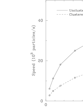
Figure 8: Code speed in thousands of particles per second as a function of number of processors for both smooth and clustered positions for a small $2\times 64^{3}$ particle combined gas and dark matter cosmological simulation

Hydra is extremely fast when the particles are unclustered. As structure forms the mean number of neighbours grows, increasing the work significantly. The amount of communication required for the parallel code also rises sharply because under CRAFT the PP calculation is expensive. The speed and scaling properties of the full code are shown in Figure 8. We plot the number of particles which can be computed per second on various numbers of processors for a small combined gas plus dark matter simulation which contained $64^{3}$ particles of each species. A problem of this size just fits on 4 T3D processors but, as shown in the figure, is too small to scale well above 32 processors. The plot gives timings both for the initial smooth distribution and for a highly evolved position at a redshift of 0.5. Rates for larger gas-plus-dark matter runs with $2\times 128^{3}$ particles on 256 processors have been measured at $6.6\times 10^{4}$ particles per second unclustered, dropping to $1.1\times 10^{4}$ particles per second under very heavy clustering. In runs with only dark matter with $256^{3}$ particles we have achieved peak rates of $3.3\times 10^{5}$ particles per second on 256 processors unclustered, and, under moderate clustering, $6.8\times 10^{4}$ particles per second on 128 processors and $8.4\times 10^{4}$ particles per second on 256 processors.

4.3 Load Balance

Initially the load balance is very good because there is very little PP work and the PM section is well balanced. Once clustering develops we encounter three problems. Firstly, some of the PP cells take a long time to complete and even with the very fine grained balancing employed by the PP routine there is an imbalance while one processor finishes a particularly difficult cell (see Figure 6). Secondly, the large refinements that are done in parallel across the full machine are really too small to be done in this way (but too big for a single processor). The maximum number of processors that should be used for the FFT routine is $L_{\rm mesh}$, the size of the PM grid. In practice, $L_{\rm mesh}=64$ for these refinements and the time taken does not scale well if more than 32 processors are used. CRAFT does not have a facility that would allow the assignment of a subset of the processors to a task, being limited to either using all the processors or just one processor. Finally, a refinement cannot be started before its parent has been completed. This means that the small refinements cannot all be completed as a single task farm but must be done one level at a time. Unfortunately, the time then scales as the sum of the times of the most expensive refinement at each level. As shown in figure 7 this leads to a load imbalance while one processor finishes the most difficult refinement at each level.

Table 1 gives the relative timings for the main sections of the code on a typical clustered step within a $2\times 128^{3}$ particle combined gas and dark matter cosmological simulation. Over half of the time is spent in the PP routine at the top-level. There are four levels of refinement. The single fourth-level refinement takes longer than the 17 third level ones combined because 64 processors are available so these all execute in parallel. The biggest saving in terms of load balance could be achieved in the PP routine where perhaps 100 seconds of the nearly 300 second step could be saved if it was possible to either split up individual PP cells over several processors or to place the refinements so that these cells are avoided.

Routine		Subroutine		Number
Top level	66.8			1
		$PP$	55.9
		$PM$	6.78
		list sort	3.30
		placing refinements	0.81
Big refinements	14.0			3
		1	3.77
		2	5.06
		3	5.17
Small refinements	19.2
		level 1	12.6	358
		level 2	4.66	182
		level 3	0.83	17
		level 4	1.08	1

Table 1: Percentage time required by different coarse grained sections of the code, taken from redshift 0.5 in a $2\times 128^{3}$ particle combined gas and dark matter run

4.4 Memory requirements

The number of words of storage required by Hydra is,

$$N_{\rm words} = 2(L_{\rm max}^{3}+2L_{\rm pmax}^{3}+2N_{\rm pes}L_{\rm rmax})+$$

$$19(N_{\rm max}+N_{\rm pmax}+N_{\rm pes}N_{\rm rmax})+5N_{\rm pes}n_{\rm max},$$

where, $L_{\rm max}$ is the maximum size of the top level PM mesh, $L_{\rm pmax}$ is the maximum size of the parallel refinement meshes, $L_{\rm rmax}$ is the maximum size of the small (task-farmed) refinement meshes, $N_{\rm pes}$ is the number of processors, $N_{\rm max}$ is the maximum number of particles, $N_{\rm pmax}$ is the maximum number of particles within a parallel refinement, $N_{\rm rmax}$ is the maximum number of particles within a small refinement and $n_{\rm max}$ is the maximum number of PP neighbours allowed.

Figure 9: Memory usage of parallel Hydra for several different values of $N$. We are capable of running a 100 million particle gas and dark matter run on a 512 processor T3D.

Typically we set, $L_{\rm max}=2N_{\rm max}^{1\over 3}$, $N_{\rm pmax}=128^{3}$, $L_{\rm pmax}=128$, $N_{\rm rmax}=32^{3}$, $L_{\rm rmax}=32$ and $n_{\rm max}=64^{3}/2$. Figure 9 shows a plot of the memory requirements of the code for various values of $N$ against number of processors. There are $64\,$ Mb of memory available per processor on the T3D in Edinburgh. Equation 2 is a good measure of the memory usage because the 16.8 million particle simulation does in fact run on 128 processors.

These figures are for the full SPH code. Without gas the storage requirement can be reduced substantially. In this case the number of arrays needed to store the particle properties can be reduced from 19 to 13 trivially and even further to 7 if the timestepping scheme is modified.

5 Summary

A parallel adaptive grid code based on Couchman’s (1991) algorithm has been implemented on the Cray T3D using CRAFT. We have incorporated SPH following the prescription of Couchman, Thomas & Pearce (1995). The code, Hydra, is capable of running $2\times 64^{3}$ particle combined cooling gas and dark matter cosmological simulations in $\sim 600$ processor hours. These runs are very useful for exploring parameter space in order to target larger $2\times 128^{3}$ particle runs. We have completed a sequence of these, the results of which will be presented elsewhere (e.g., Pearce et al. 1997).

The parallel version of Hydra can also be used for more traditional dark matter only simulations. We have completed a series of $256^{3}$ (16.8 million) particle models in a variety of cosmologies (Thomas et al. 1997, Jenkins et al. 1997). Parallel Hydra was also used as part of the recent cluster comparison exercise (Frenk et al. 1997) where many different hydrodynamic codes where used to perform the same simulation.

References

Aarseth, S. J., 1963, MNRAS, 126, 223

Appel, A., 1985, SIAM J. Sci. Stat. Comp., 6, 85

Barnes, J. E., Hut, P., 1986, Nat, 324, 446

Cole, S., Lacey, C., 1996, astro-ph/9510147

Couchman, H. M. P., 1997, In Proceedings of the 12th Kingston Meeting on Theoretical Astrophysics, eds. Clarke, D. and West, M.

Couchman, H. M. P., 1991, ApJ, 368, L23

Couchman, H. M. P., Thomas, P. A., Pearce, F. R., 1995, ApJ, 452, 797

Davé, R., Dubinski, J., Hernquist, L., 1997, astro-ph/9701113

Dubinski, J., 1996, NewA, 1, 133

Efstathiou, G., Davis, M., Frenk, C. S., White, S. D. M., 1985, ApJS, 57, 241

Efstathiou, G., Frenk, C. S., White, S. D. M., Davis, M., 1988, MNRAS, 235, 715

Efstathiou, G., Eastwood, J. W., 1981, MNRAS, 194, 503

Evrard, A. E., 1990, ApJ, 363, 349

Ferrell, R., Bertschinger, E., 1994, Int. Jour. Mod. Phys. C, 5, 933

Ferrell, R., Bertschinger, E., 1995, In Proceedings of the 1995 Society for Computer Simulation Multiconference

Frenk, C. S. et al. , 1997, in preparation

Greengard, L., Rokhlin, V., 1987, J. Comp. Phys., 73, 325

Hockney, R. W., Eastwood, J. W., 1981, Computer Simulation Using Particles, McGraw-Hill

Jenkins, A. R., Pearce, F. R., Thomas, P. A., Frenk, C. S., Couchman, H. M. P., White, S. D. M., Colberg, J. M., Hutchings, R., Peacock, J. A., Efstathiou, G. P., Nelson, A. H., 1997, in preparation

Jernigan, J. G., 1985, In IAU Symposium No.127, ed. J. Goodman, P. Hut, pg 275, Dordrecht, Reidel

Miller, R. H., 1978, ApJ, 223, 122

Miller, R. H., Smith, B. F., 1980, ApJ, 235, 421

Monaghan, J. J., 1992, ARA&A, 30, 543

Pearce, F. R., Thomas, P. A., Couchman, H. M. P., 1993, MNRAS, 264, 497

Pearce, F. R., Thomas, P. A., Couchman, H. M. P., 1994, MNRAS, 268, 953

Pearce, F. R., Couchman, H. M. P., Jenkins, A. R., Thomas, P. A., 1995, in Dynamic Load Balancing on MPP Systems

Pearce, F. R., Thomas, P. A., Jenkins, A. R., Frenk, C. S., Couchman, H. M. P., White, S. D. M., Colberg, J. M., Hutchings, R., Peacock, J. A., Efstathiou, G. P., Nelson, A. H., 1997, in preparation

Salmon, J., 1991, PhD thesis, California Institute of Technology

Sellwood, J. A., 1987, ARA&A, 25, 251

Steinmetz, M., 1996, MNRAS, 278, 1005

Thomas, P. A., Couchman, H. M. P., 1992, MNRAS, 257, 11

Thomas, P. A., Pearce, F. R., Jenkins, A. R., Frenk, C. S., Couchman, H. M. P., White, S. D. M., Colberg, J. M., Hutchings, R., Peacock, J. A., Efstathiou, G. P., Nelson, A. H., 1997, in preparation

van Albada, T. S., van Gorkum, J. H., 1977, A&A, 54, 121

von Hoerner, S., 1960, Zeit. Ap., 50, 184

Villumsen, J. V., 1982, MNRAS, 199, 493