A comparison between Fast Multipole Algorithm and Tree–Code to evaluate gravitational forces in 3-D

Abstract

We present tests of comparison between our versions of the Fast Multipole Algorithm (FMA) and “classic” tree–code to evaluate gravitational forces in particle systems. We have optimized the Greengard’s original version of FMA allowing for a more efficient criterion of well–separation between boxes, to improve the adaptivity of the method (which is very important in highly inhomogeneous situations) and to permit the smoothing of gravitational interactions.

The results of our tests indicate that the tree–code is almost three times faster than FMA for both a homogeneous and a clumped distribution, at least in the interval of $N$ ($N\leq 10^{5}$) here investigated and at the same level of accuracy (error $\sim 10^{-3}$). This order of accuracy is generally considered as the best compromise between CPU–time consumption and precision for astrophysical simulation. Moreover, the claimed linear dependence on $N$ of the CPU–time of FMA is not confirmed and we give a “theoretical” explanation for that.

running head: FMA and Tree–Code comparison

send proofs to:

R. Capuzzo–Dolcetta

Istituto Astronomico, Universitá La Sapienza

via G.M. Lancisi 29, I-00161, Roma, Italy

e–mail: dolcetta@astrmb.rm.astro.it

1 Introduction

The availability of fast computers is allowing a huge development of simulations of large $N$–body systems in Astrophysics, as well as in other fields of physics where the behaviour of large systems of particles have to be investigated.

The heaviest computational part of a dynamical simulation of such systems (composed by point masses and/or smoothed particles representing a gas) is the evaluation of the long–range force, such as the gravitational one, acting on every particle and due to all the other particles of the system. Astrophysically realistic simulations require very large $N$ (greater than $10^{5}$), making the direct $\sim N^{2}$ pair gravitational interaction evaluations too slow to perform. To overcome this problem various approximated techniques to compute gravitational interactions have been proposed.
Among them, the tree–code algorithm proposed by Barnes & Hut (hereafter B.H., see [BH ]) is now widely used in Astrophysics because it does not require any spatial fixed grid (like, for example, methods based on the solution of Poisson’s equation). This makes it apt to follow very inhomogeneous and variable in time situations, typical of self–gravitating systems out of equilibrium. In fact its intrinsic capability to give a rapid evaluation of forces allows to dedicate more CPU–time to follow fast dynamical evolution, contrarily to other higher accuracy methods that are more suitable in other physical situations, e.g. molecular dynamics for polar fluids, where Coulomb term is present.

While for the tree–code the CPU–time requirement scales as $N\log_{8}N$, in the recently proposed Fast Multipole Algorithm (hereafter FMA, see [greengard ]) this time is claimed to scale as $N$, at least in quasi–homogeneous 2–D particle distributions. Were this linear behaviour confirmed in 3-D highly non–uniform cases, FMA would really be appealing for use in astrophysical simulations.
In this paper, we compare CPU times of our own implementations of adaptive 3-D FMA and tree–code to evaluate gravitational forces among $N$ particles in two rather different (uniform and clumped) spatial configurations.

Detailed descriptions of tree–code and FMA can be found in [BH ], [H ] and [greengard ] respectively. For the purpose of this paper (the performance comparison of the two above mentioned methods in astrophysically realistic situations) we built our own computer versions of tree–code and FMA. Our tree–code was written following at most the [HK ] prescription but for the short–range component of the interaction force (see [tesi ]), while our FMA is slightly different from the original proposed by Greengard [greengard ], to make it more efficient in non–uniform situations where adaptivity is important, and to include the smoothing of interactions which is quite useful in astrophysical simulations, as we will describe in Sect. 3.

In Sect. 2 and 3 we briefly review the algorithms and give some details of our implementations, in particular for the FMA, while in Sect. 4 the comparison of FMA and tree–code CPU–time performances is presented and discussed.

2 The tree–code

We have implementated our own version of the “classic” BH tree–code (see [BH ] or [H ]) which is well described in [tesi ] (see also [HK ]); we will give here only a brief discussion of the improvements we have introduced.

In the tree–code the cubic volume of side $\ell$ that encloses all the particles is subdivided in 8 cubic boxes (in 3-D) and each of them is further subdivided in 8 children boxes and so on. The subdivision goes on recursively until the smallest boxes (the so called terminal boxes) have only one particle inside. Moreover the subdivision is local and adaptive in the sense that it is locally as more refined as the density is higher. The logical internal representation of this picture is a “tree data structure”, from that the denomination tree–code.

The gravitational force on a given particle in $\bf r$ is then computed considering the contribution of the “clusters” of particles contained in boxes that are sufficiently distant from the particle, that is in those boxes which satisfy the open–angle criterion:

$$\frac{\ell_{m}}{d}<\theta$$ (1)

with $d$ the distance between the particle and the center of mass of the cluster, $\ell_{m}=\ell/2^{m}$ the box size at level $m$ of refinement and $\theta>0$ a parameter a priori fixed. This contribution is evaluated by means of a truncated multipole expansion that permits to represent the set of $n$ particles contained in the box with a unique “entity” identified by a relatively low number of attributes (the total mass, the center of mass, the quadrupole moment…, that is the set of multipole coefficients), that are stored, in a previous step, in the tree data structure. In this way the evaluation of interactions is speeded–up compared to a direct pair-to-pair evaluation. Usually in tree–codes second order expansions are used, that is up to the quadrupole term, this approximation being sufficient in typical astrophysical simulations. Those boxes that do not satisfy the condition (1), will be “opened” and their children boxes will be considered. This “tree descending” continues until one reaches a terminal box whose contribution to the field will be calculated directly.

The parameter $\theta$ and the order of truncation of the expansion, permit to have some control of the error made in the evaluation of the field in the generic particle position. With the second order of approximation we used and with $\theta$ in the interval $[0.7,1]$ one obtaines a relative error less then about 1%, as we will see in the following.

In our version of the tree–code we considered a gravitational smoothing. This means that each particle is represented by a $\beta$-spline (a polinomial function, with a compact support, differentiable up to the second order) that gives a Newtonian potential outside the sphere centered at the position of the particle and of radius $2\epsilon$, while inside that sphere the field is smoothed; see for example [HK ] and [tesi ]. This smoothing avoids divergence in the accelerations during too close approaches between particles whose trajectories would be not well integrated in time by the usual numerical procedures (like, for example, the leap–frog scheme). In the particular case of our static test, i.e. without considering any time evolution, the smoothing would only be an unnecessary complication; consequently in these tests we fix $\epsilon=0$ for every particle (exactly Newtonian potential).

However because of the presence, in general, of a smoothing of the field we have modified the open–angle criteria in the following way: the box of size $\ell$ with center of mass at $\bf R$ is “sufficiently distant” from the particle in $\bf r$, i.e. its potential can be expandend in a multipole series, if

$$|{\bf R}-{\bf r}|>\max\{\ell/\theta,2\epsilon\}$$ (2)

where $2\epsilon$ is the gravitational smoothing “radius” of the particle in $\bf r$.

3 The Fast Multipole Algorithm

In a way similar to the tree–code, the FMA is based on an approximation of the gravitational field produced by a set of sufficiently distant particles over a generic particle. It uses the same logical “octal tree–structure” of the hierarchical subdivision of the space as the tree–code, with the only difference that instead of stopping subdivision when boxes contain single particles, in this case the recursive subdivision ends up at boxes containing no more than a fixed number $s>1$ of particles. This to reduce the CPU–time required for the calculation. We still call terminal boxes the boxes located at the “leaves” of the logical tree–structure. Also the FMA uses the truncated multipole expansion, but in a different and more complicated form. The advantage is that of a more rigorouse control of the truncation error.

In general the spherical harmonics expansion works for particles interacting via a potential $\Phi({\bf r},{\bf r}^{\prime})\propto 1/|{\bf r}-{\bf r}^{\prime}|$, so, even if we will always speak in terms of gravitational field the treatment is the same in the case of electrostatic field. The only differences are the coupling constant and the attribute of each particle (the mass in the gravitational case, the charge with its sign in the electrostatic case).

The FMA takes advantage of that if we know the coefficients of the multipole expansion that gives the potential in a point $P$, we are able to build a Taylor expansion —the so called local expansion— of the potential in a neighbourhood of $P$ (see Appendix A). This expansion is used to evaluate the acceleration of a particle near $P$, instead of re-evaluating the multipole expansions of the field due to all collections of distant particles as it happens with the tree–code.

Furthermore, besides the interaction particle–particle and particle–box, FMA considers also an interaction box–box which is estimated by a truncated multipolar expansion, if and only if the boxes are sufficiently distant one each other, that is if they satisfy the so called well–separation criterion (which substitutes the open–angle criterion of the tree–code). Boxes which are not well–separated, will be “opened” and their children boxes considered. In this way one can control the error introduced by the truncation of the multipolar expansion, having this error, as we will see, a well defined upper bound.

In fact we know that, if we have a set of $k$ particles at $P_{i}=(\rho_{i},\alpha_{i},\beta_{i})$ (we will use spherical coordinates) having masses $m_{i}$, which is enclosed in a sphere $A$ with center in the origin and radius $a$, and another set of $l$ particles at $Q_{i}=(r_{i},\theta_{i},\phi_{i})$ enclosed in a sphere $B$ centered in $Q_{0}$ with radius $b$, then the approximated potential generated by the set of particles in $A$ at the position of the $i$-th particle in $B$, is given by a multipole expansion truncated at the order $p$:

$$\tilde{\Phi}_{p}(Q_{i})\equiv-G\sum_{n=0}^{p}\sum_{m=-n}^{n}\frac{M^{m}_{n}}{r^{n+1}_{i}}Y^{m}_{n}(\theta_{i},\phi_{i}).$$ (3)

The functions $Y^{m}_{n}(\theta,\phi)$ are the spherical harmonics and

$$M^{m}_{n}\equiv\sum_{i=1}^{k}m_{i}\rho_{i}^{n}Y^{-m}_{n}(\alpha_{i},\beta_{i}).$$ (4)

Now one can show (see [greengard ]) that, for any $p\geq 1$,

$$|\Phi(Q_{i})-\tilde{\Phi}_{p}(Q_{i})|\leq\frac{{\cal A}}{r_{i}-a}\left(\frac{a}{r_{i}}\right)^{p+1},$$ (5)

where $\Phi$ is the exact potential and ${\cal A}\equiv G\sum_{i=1}^{k}m_{i}$. This result gives the possibility to limit the error introduced by approximating $\Phi$ with the expression (3), if the two sets of particles are sufficiently distant.

Let $d$ be the distance between the centers of the two spheres and let us define $\sigma\equiv d-a-b$ the separation between them. Obviously the set of particles in $B$ is such that $r_{i}\geq a+\sigma$ for any $i=1,...,l$. Then from (5) we find:

$$\Delta\Phi\equiv\max_{i=1,...,l}\left\{|\Phi(Q_{i})-\tilde{\Phi}_{p}(Q_{i})|\right\}\leq\frac{{\cal A}}{\sigma}\left(\frac{a}{\sigma+a}\right)^{p+1}.$$ (6)

The maximum error of the truncated multipole expansion depends on two quantities: the order of the expansion $p$ and the separation $\sigma$.

In his original algorithm, Greengard introduced the concept of well–separation between two boxes of the same level of refinement, i.e. with the same size $\ell$, to control the truncation error. Suppose to have two sets of particles in two boxes circumscribed by two spheres $A$ and $B$, with equal radii $a=b=\ell\sqrt{3}/2$: these two boxes are well–separated if, and only if, their separation is such that $\sigma>a$, i.e. $d>3a$. In this way the upper bound on the error will be, from eq. (6),

$$\Delta\Phi\leq\frac{{\cal A}}{a}\left(\frac{1}{2}\right)^{p+1}.$$ (7)

To implement this criterion, Greengard imposed simply that: two boxes of the same level are well–separated if, and only if, there are at least two layers of boxes of that level between them, in such a way to satisfy the inequality $d>3a$ and finally the (7).

Note that Greengard’s well–separation criterion refers exclusively to boxes at the same level of refinement, limiting the efficiency of the algorithm especially in the case of non–uniform distributions of particles.

We have modified this criterion to make it more efficient (in the adaptive form of the algorithm) to face astrophysical typical distributions very far from uniformity.
Let us briefly explain our modification.
First of all, every box is associated to a sphere that is not merely the sphere circumscribing the box but the smallest one containing all its particle. So, for terminal boxes, is the smallest sphere concentric to the box and that contains all its particles and for a non–terminal box of size $\ell$, the sphere is also concentric to the box but the radius $r$ is calculated recursively, knowing the radii $r_{i}$ $(i=1,...,8)$ of the spheres associated to each of its children unempty boxes, via the formula

$$r=\max_{i=1,...,8}\{r_{i}\}+\ell\sqrt{3}/2.$$ (8)

This sphere contains all the spheres associated to the children boxes . The value of the radius of these spheres is stored in the “tree” data structure together with the other data pertinent to the box and it is much more representative of the “size” of the set of particles in the box, than the mere box size $\ell$, for controlling the truncation error.

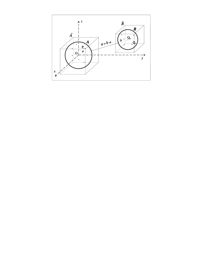
Figure 1: Example of two well–separated boxes, $\hat{A}$ and $\hat{B}$ (see text). $A$ and $B$ are the associated spheres enclosing the two set of particles.

Now consider the box $\hat{A}$ centered in the origin $O$ and containing the collection of $k$ particles belonging to the sphere $A$ seen before. Let this sphere $A$ be its associated sphere with radius $a$ (see Fig. 1). Let the other set of particles at $Q_{i},i=1,..,l$, be enclosed in the box $\hat{B}$ whose associated sphere be the sphere $B$ centered in $Q_{0}$ and with radius $b$. The radii $a,b$ have been evaluated by the (8). Let us suppose that the separation of the two spheres is such that $\sigma>\delta\cdot a$, with $\delta>0$ a fixed parameter (see again Fig.1). Obviously the set of particles in $B$ is such that, from eq. (6),

$$\Delta\Phi\leq\frac{{\cal A}}{\delta\cdot a}\left(\frac{1}{\delta+1}\right)^{p+1}$$ (9)

and we can note that the parameter $\delta$ works in a way similar to $\theta$ in the tree–code.

Hence, our criterion of well–separation is the following: once we fixed the parameter $\delta$, we define two boxes as well–separated, if the distance between their centers $d$ is such that

$$d>a+b+\delta\cdot a,$$ (10)

that is if the separation between their associated spheres is $\sigma>\delta\cdot a$. In this way the evaluation of the interaction between the sets of particles contained into such boxes will be affected by a truncation error which is bounded by the (9).

The implementation of this criterion is very easy because it consists just in verifying the (10) where the radii of the spheres associated to the boxes have been already calculated and stored, together with all the other data of each box, in the phase of the algorithm in which the tree–structure is built.

Our criterion of well–separation is more efficient than the Greengard’s original one, having the following features:

• it depends upon the internal distribution of particles in the box (via the radius of the associated sphere);

• it can involve boxes of different level of refinement, having different sizes, so to improve efficiency in non–uniform situations and to make unnecessary those complicated tricks conceived to shorten the list of the well–separated boxes like, for example, the mechanism of “parental conversion”, (see [board ]);

• it can be tuned in such a way to obtain the desired accuracy, via the parameter $\delta$;

• it can be easily modified in order to allow a gravitational smoothing to be applied to the particles, as we will see below.

Note also, see the (7), that to control the truncation error, Greengard varied $p$ according to the desired accuracy. In our version we have, instead, fixed $p=2$ and achieved varied the parameter $\delta$ in order to obtain the same accuracy that is usually obtained with the tree–code in astrophysical simulations. One has to care with keeping reasonably low the execution CPU–time (be small compared with human time scale!) and this is obtained at a price of a certain loss in accuracy in the evaluation of interactions. In fact the main characteristics of astrophysical simulations of gravitating systems are:

1. they require a great number of particles (usually more than $10^{4}$) for a rather large duration of the simulation and, in particular,

2. due to the intrinsic instability they offer a very wide distribution of time scales.

So while simulating polar fluids in molecular dynamics, one has to face “microscopic” time scales more narrowly distributed (just because molecules tend to repulse each other due to the presence of short–range interactions, like the Lennard–Jones potential) and one can work with expansions truncated up to eighth order or more (although the CPU–time grows as $p^{4}$, see [greengard ]), in astrophysical simulations one prefers to limit the precision at a lower but reasonable level and, on the other hand, to be able to process systems which are highly dynamical. Therefore one usually works with expansions truncated up to the second order (in some cases even the first order) that, in the tree–code, corresponds to consider up to the quadrupole moment.

For the mass density of the single particle we used the same $\beta$–spline profile as we did in our tree–code. In this way the potential is exactly Newtonian outside the sphere of radius $2\epsilon_{i}$ centered in ${\bf r}_{i}$, so it can be expanded in multipole series only in this region. Hence the interaction with a particle inside the sphere of radius $2\epsilon_{i}$ must be necessarily evaluated by means of a direct summation. This requirement, which would be very difficult to incorporate in Greengard’s criterium, has been considered via a little arrangement of our well–separation criterium (10), that is:
two boxes ($\hat{A}$ and $\hat{B}$) are well–separated if, and only if, their spheres ($A$, with radius $a$ and $B$ with radius $b$ respectively) are such that:

$$d\geq a+b+\max\{\delta\cdot a,2\epsilon_{\hat{A}}\}$$ (11)

where $d$ is the distance between the centers of the two spheres.

The smoothing length $\epsilon_{\hat{A}}$ used for the box $\hat{A}$ is another quantity stored in the tree data structure and it is given by this simple recursive scheme: if $\hat{A}$ is terminal, then $\epsilon_{\hat{A}}\equiv\max_{i}\{\epsilon_{i}\}$, where $\epsilon_{i}$ is the smoothing lenght of the particle $i$ contained in $\hat{A}$, otherwise $\epsilon_{\hat{A}}\equiv\max_{\hat{C}}\{\epsilon_{\hat{C}}\}$, with the maximum taken over all the unempty children boxes $\hat{C}$ of $\hat{A}$. Anyway in the following comparison tests, we let $\epsilon=0$ (as for the tree–code) because we are not interested in the dynamical evolution of the system.

For a more detailed description of our own implementaton of FMA see Appendixes A and B.

4 Codes performance comparison

To compare the CPU–time spent by the two algorithms described in the previous Sections, we ran the codes on a IBM R6000 workstation with two different distributions of particles. In the first case $N$ particles have been distributed a uniformly at random in a sphere of unitary radius. In the second case a set of $N$ particles has been distributed, with a Monte–Carlo method, in a unitary sphere in such a way to discretize the density profile:

$$\rho(r)=\frac{\rho_{0}}{\left[1+\left(\frac{r}{r_{c}}\right)^{2}\right]^{5/2}},$$ (12)

with $r_{c}=0.2$ (obviously $\rho=0$ for $r>1$). This latter is known as Schuster’s ([schuster ]) profile; it corresponds to a polytropic sphere (of index 5) at equilibrium (see [Binney ]) and represents a good approximation to the density distribution of various stellar systems. In both the uniform and clumped case all the particles are assumed to have the same mass.

The order of accuracy chosen was the same for both the tree–code and the FMA. For accuracy we mean how close, in modulus, the evaluated forces are to those calculated “exactly” by a direct, Particle–Particle (PP) method, which is affected only by the numerical error of the computer (due to the finite number of digits). Consequently we define as relative error of the calculation $\varepsilon$:

$$\varepsilon\equiv\frac{1}{N}\sum_{i}^{N}\frac{|a_{i}-a^{PP}_{i}|}{a^{PP}_{i}},$$ (13)

where $a_{i}$ is the modulus of the acceleration of the $i$-th particle estimated by each of the two algorithms and $a^{PP}_{i}$ that computed by the PP method. The error on the direction of the forces is much lower then the error on the modulus we have defined above, and, as it is usual in N–body numerical method, it is not considered at all in performance tests being negligible.

Figure 2: Averaged relative error vs. number of particles for both algorithms.

Figure 3: CPU–time (on an IBM R6000 machine) vs. number of particles for both the algorithms and for the direct Particle–Particle method.

Figure 2 gives the relative error of the tree–code and of the FMA in the uniform and “clumped” case. The error is almost the same for both the algorithms. An averaged (on all the particles) relative error less than 1% (this is the order of magnitude of the error generally admitted in astrophysical simulations), is obtained fixing

$$\theta = 0.7\mbox{ for the tree--code,}$$ (14)

$$\delta = 2.5\mbox{ for the FMA},$$ (15)

and considering, as we have said, up to the quadrupole term in the tree–code and to the same order term in the multipole expansion ($p=2$) of the FMA. Moreover we chose $s=10$ in the FMA as the best compromise between accuracy and computational speed, as we checked.

The CPU–time spent to calculate the accelerations vs. the number $N$ of particles is shown in Fig.3. The CPU–time for the Particle–Particle method is also shown as reference. Both the algorithms are slower to compute forces in the non–uniform model than in the uniform one, and for the tree–code this is more evident. This is clearly due to the more complicated and non-uniform spatial subdivision in boxes that affects mostly the tree–code due to the finer and deeper subdivision of the space it uses. Anyway the tree–code shows to be faster than the FMA for both the distributions and for $N$ varying in the range we tested. As expected, the behaviour of the CPU–time vs. $N$ for the tree–code is well fitted by the logaritmic law

$$t_{cpu}=\alpha N\log N+\beta,$$ (16)

where $\alpha$ and $\beta$ are given in Table 1. In our opinion, this law must be followed by the FMA too, as we will explain in Section 4.1.

However, let us observe the CPU–time for the uniform case: it is not easy to distinguish at a first sight a logarithmic behaviour from a linear one, furthermore we can presume, as we can observe in Figure 3, that the FMA must show a more complicated behaviour due to the presence of the parameter $s$ (the maximum number of particles leaved in terminal boxes) and to that $s$ was kept fixed. Hence for a certain range of $N$ this $s$ could have been chosen as optimum, but could have not been so for other values of $N$ (in those ranges in which the CPU–time shows to grow excessively with a slope larger than that of the tree–code and comparable to that of the PP method). Blelloch and Narlikar [BN ] have obtained similar “undulations” in the behaviour of the CPU–time of their version of FMA, while the behaviour of tree–code was much “cleaner”, as in our tests.

Coming back to the accuracy, note that for $N>8192$, the rel. error of the FMA exceeds that of the tree–code (see Fig.2). In the same range of $N$ the CPU–time of the FMA grows less rapidly than that of the tree–code. This follows the obvious gross rule by which the faster the calculation the lower the precision in the results. So for $N>8192$ the value $s=10$ fixed is likely too small and consequently the percentage of direct (PP) calculation is decreased, so that FMA loses precision. On the contrary, for $N<4096$ we observe, especially in the Schuster case, that $\varepsilon_{FMA}<\varepsilon_{tc}$; in the same region the CPU–time for FMA grows more rapidly than for the tree–code, so in this case $s$ seems to be too high.

Uniform	Schuster
Algorithm $\alpha$ $\beta$ tree–code $1.1\cdot 10^{-3}$ $-1.1$ FMA $4\cdot 10^{-3}$ $-7.4$	Algorithm $\alpha$ $\beta$ tree–code $1.6\cdot 10^{-3}$ $-1.7$ FMA $4.9\cdot 10^{-3}$ $-10$

Table 1: Values obtained for the parameter, fitting the behaviour of the CPU–time for both algorithms with the law: $t_{cpu}=\alpha N\log_{8}N+\beta$.

It is interesting to note that the relative error of the tree–code shows a decrease at increasing the number of particles. This is probably due to the large fraction of direct, particle–particle calculations, because of the growing density of particles (the volume occupied by the system remains the same). This explains also the lower error in the clumped case than in the uniform one at a given $N$, because in the Schuster’s profile the central density of particles is clearly higher than in the uniform case.

Finally we can see that our FMA becomes faster than the PP method for $N>18,000$ in the Schuster’s model, and for $N>16,000$ in the uniform case.
To make a comparison with codes of other authors, let us consider the FMA implemented in 3-D by Schmidt and Lee [SL ] (although this code is not adaptive) following the original Greengard’s algorithm and, in particular, his well–separation criterion. Their FMA is vectorized and it runs on a CRAY Y-MP, but anyway we do not make a direct comparison, but rather compare our “CPU–time ratio” (that is the ratio between the CPU–time consumed by FMA and that consumed by the direct PP method), with the same ratio as obtained by the codes of Schmidt and Lee, at the same order of magnitude of the error on the forces.

So we can note (see [SL ]) that for $N=10^{4}$ uniformly distributed particles, a truncation of eighth order ($p=8$) and five levels of refinement (a priori chosen), they obtain a CPU–time of 418 sec. for their FMA, against 11 sec. spent by the direct PP method, with a relative error on the forces of about $1.4\cdot 10^{-3}$. Thus they obtain a ratio $t_{cpu}^{(FMA)}/t_{cpu}^{(PP)}\sim 40$, while with our codes we see that for the uniform distribution with $N=10^{4}$, we have an error on the forces that is $\sim 3\cdot 10^{-3}$ (see Fig.2) with a CPU–time ratio $t_{cpu}^{(FMA)}/t_{cpu}^{(PP)}\sim 1$, i.e. about the same CPU–time spent by the PP method (see Fig.3).

This seems a very good result.

4.1 Scaling of CPU–times versus $N$

Greengard and other authors ([greengard ], [board ],[salmon ]) assert that FMA would exhibit a linear scaling of CPU–time vs. $N$. We tried to fit $t_{cpu}^{(FMA)}$ as function of $N$, with various laws, the linear included. The result is that a logarithmic behaviour like that of eq. (16), gives the best fit, as for the tree–code.

The values obtained for $\alpha$ and $\beta$ in Table 1 show that $\alpha_{FMA}/\alpha_{tc}\sim 3$: the tree–code is roughly three times faster than the FMA. Note how this difference of performances reduces slightly passing to the Schuster clumped profile; this because, as we have said, our FMA adaptive code is less sensitive to the degree of uniformity of the distribution of the particles than the tree–code which uses a finer subdivision of the space in boxes (as it corresponds to $s=1$).

The higher speed of the tree–code respect to the FMA is easily understood, at least in 3-D, since while in theory the FMA is more efficient and less “redundant” in managing informations (remember the use of Taylor expansion of the potential on near bodies), in practice this “potential” greater efficiency pays the price of a certain quantity of computational “complications”. This carries the method to a negative total balance in terms of speed respect to the competing tree–code.

How can we interpret the CPU–time scaling?
The logarithmic behaviour of the tree–code is explained by a simple estimate of the number of operations needed by the various steps of the algorithm (see e.g. [BH ],[H ] and [tesi ]). It is roughly given by the product between the number of particles $N$ by the number of “bodies” (boxes or particles), about $\log_{8}N$, which contribute to the force on each particle. Hence $t_{cpu}^{(tr)}\sim N\log_{8}N$.

The logarithmic behaviour of the FMA can be similarly understood when one reconsiders carefully the cost of each step of the algorithm.
It can be estimated (see [greengard ]) that

$$t_{cpu}^{(FMA)}\sim aN+bN_{ter}+cN_{ne},$$ (17)

that is the CPU–time is a linear function of $N$, $N_{ter}$ (the number of all terminal boxes) and $N_{ne}$ (the number of all non–empty boxes). Greengard [greengard ] in his final considerations on the scaling of the FMA in the adaptive 2-D version (the 3-D case is similar), estimates the number of this types of boxes (see lemmas 2.6.4 and 2.6.5 in [greengard ]) to be

$$N_{ter} \sim 4\cdot L\cdot\frac{N}{s}$$ (18)

$$N_{ne} \sim 5\cdot L\cdot\frac{N}{s}$$ (19)

where $L$ is the total number of subdivisions needed to reach terminal boxes. This $L$ is identified by Greengard with $L\sim\log_{2}(1/\Delta)$, where $\Delta$, a priori fixed, is the spatial resolution that one wants to reach in the simulation. Being $\Delta$ fixed, $L$ would be independent of $N$, thus $N_{ter}$ and $N_{ne}$, in eq. (17), are quantities linear in $N$. Then the FMA CPU–time estimated by the eq. (17) results linear in $N$ too.

The crucial point is that a constant $\Delta$ (and $L$) allows to manipulate only those distribution of particles such that $\Delta<r_{min}$, with $r_{min}$ the minimum distance between a pair of particles (see observation 2.5.1 in [greengard ]).

Obviously, in 3-D, $r_{min}\sim N^{-1/3}$, so that $\Delta<r_{min}$ implies

$$L\mathop{\vtop{\halign{#\cr$\hfil\displaystyle{>}\hfil$\crcr\kern 1.0pt\nointerlineskip\cr\hbox{$\hfil\sim\hfil$}\crcr\kern 1.0pt\cr}}}\frac{1}{2}\log_{2}N=\log_{8}N$$ (20)

Substituting this inequality in the expressions (18) and (19) for $N_{ne}$ and $N_{ter}$, one obtains from eq. (17) that $t_{cpu}^{(FMA)}\mathop{\vtop{\halign{#\cr$\hfil\displaystyle{>}\hfil$\crcr\kern 1.0pt\nointerlineskip\cr\hbox{$\hfil\sim\hfil$}\crcr\kern 1.0pt\cr}}}N\log_{8}N$, that is the same “natural” scaling of the tree–code.

5 Conclusions

Realistic astrophysical simulations are characterized by the large amount of computations required by the evaluation of gravitational forces. Many codes which give performant approximation of the force field have been proposed in the literature. In this paper we compare two of these codes: one (the BH tree–code) has been largely used in astrophysics for ten years, the other (the Greengard’s FMA [greengard ]) has given promising results in the field of molecular dynamics.
We have so implemented our own optimized serial versions of both the tree–code and adaptive, 3-D, FMA.

The results of our comparison tests indicate the tree–code as faster than FMA over all the interval of total number of particles ($N\leq 10^{5}$) allowed by the central memory capacity of a “typical” workstation. This maximum value of $N$, which could appear low respect to modern parallel simulations (up to $N\sim 10^{7}$), is anyway meaningful because even fully parallel codes are limited by an individual processor charge of that order of magnitude. The problems in the parallelization of the two codes are comparable due to their similar structure, thus the higher speed of the tree–code, here verified in a serial context, should be confirmed in the parallel implementation and it seems a valid reason to concentrate efforts for the most efficient parallelization of the tree–code.

At the end of this paper we have discussed the dependence of the FMA CPU–time on $N$ and given explanation of why its behaviour is similar to that of the classic tree–code.

Appendix A Manipulation of Multipole Expansions in the FMA

Here we briefly describe the three theorems, due to Greengard [greengard ], that permits the manipulation, in 3-D, of the various series expansions used in the algorithm, and that are useful for the deeper and formal description of our own implementation that follows in the next Appendix B.

We have said that one can “transform” the multipole expansion (3) into a local expansion useful to evaluate the field about a given point $P$. More precisely, given the set of $k$ particles at $P_{i}$ in the sphere $A$ (associated to the box $\hat{A}$, see the Fig. 1) which produce the gravitational potential $\Phi(Q_{i})$ over the set of particles in the sphere $B$ (box $\hat{B}$) with center $Q_{0}$, then one can show that in the vicinity of $Q_{0}$ the approximated potential

$$\Psi_{p}(Q_{i})=-G\sum_{j=0}^{p}\sum_{k=-j}^{j}L_{j}^{k}Y_{j}^{k}(\theta^{\prime}_{i},\phi^{\prime}_{i})(r^{\prime}_{i})^{j},$$ (A1)

where $Q_{i}-Q_{0}=(r^{\prime}_{i},\theta^{\prime}_{i},\phi^{\prime}_{i})$, differs from the exact $\Phi(Q_{i})$ of an amount bounded by the same expression that appears in the r.h.s. of the eq. (9). In this truncated local expansion the coefficients are given by:

$$L_{j}^{k}=\sum_{n=0}^{p}\sum_{m=-n}^{n}S_{j,k,n,m}^{(1)}M_{n}^{m}Y_{j+n}^{m-k}(\alpha_{i},\beta_{i})(\rho_{i})^{-j-n-1},$$ (A2)

$M_{n}^{m}$ being the same that appears in the expression (3) and $S^{(1)}$ a matrix of coefficients (see Appendix C).

Another theorem allows us to calculate $M_{n}^{m}$ in a recursive manner. Let us consider the partition of the set of $k$ particles in the box $\hat{A}$, in the $q\leq 8$ sub–sets each of them enclosed in the spheres associated to the children boxes of $\hat{A}$ and with centers in $(\rho^{(1)},\alpha^{(1)},\beta^{(1)}),...,(\rho^{(q)},\alpha^{(q)},\beta^{(q)})$. Let ${M_{n}^{m}}^{(1)},{M_{n}^{m}}^{(2)},...,{M_{n}^{m}}^{(q)}$ be the multipole coefficients calculated for each of the sub–sets of particles. If all these spheres are enclosed in the sphere $A$ (this is automatically satisfied because of the eq. (8)), the coefficients $M_{j}^{k}$ given by:

$$M_{j}^{k}=\sum_{n=0}^{j}\sum_{m=-n}^{n}S_{j,k,n,m}^{(2)}{M_{j-n}^{k-m}}^{(q)}Y_{n}^{-m}(\alpha^{(q)},\beta^{(q)})(\rho^{(q)})^{n},$$ (A3)

(see the Appendix C for the matrix $S^{(2)}$) give a potential

$$\tilde{\Phi}_{p}(P)=-G\sum_{n=0}^{p}\sum_{m=-n}^{n}\frac{M^{m}_{n}}{r^{n+1}}Y^{m}_{n}(\theta,\phi)$$ (A4)

(where $P=(r,\theta,\phi)$ is a generic point outside the sphere $A$), which well approximates the exact potential $\Phi(P)$ generated by all the $k$ particles in the sphere $A$. In fact if $P$ is the position of a particle in the well–separated box $\hat{B}$, then one can show that:

$$|\tilde{\Phi}(P)-\Phi(P)|\leq\left(\frac{G\sum_{i}^{k}m_{i}}{r-a}\right)\left(\frac{a}{r}\right)^{p+1}<\frac{G\sum_{i}^{k}m_{i}}{\delta\cdot a}\left(\frac{1}{\delta+1}\right)^{p+1},$$ (A5)

the truncation error has the same upper bound given by (9).

So we can compute $M_{j}^{k}$ associated to the box $\hat{A}$ containing the total set of particles knowing only those pertinent to the $q$ sub–sets in each children box. In the tree–code the same happens, but there the analogous theorem—the “quadrupole composition theorem”—has been developed specifically for the quadrupole moment by Goldstein [Goldstein ] (those for the monopole and the dipole are obvious). In the FMA this theorem works for coefficients of any order and it has an upper error bound.

Thus, once $M_{n}^{m}$ have been calculated for all terminal boxes using the definition (4), by means of (A3) we can compute recursively the coefficients of parent boxes ascending the tree–structure. This coefficients will be transformed, when needed, in the local expansion coefficients (as we will see in more details in Appendix B) necessary to calculate forces by (A1). In this way, we will be sure that the error made in approximating the “true” potential with the various expansions, will always be bounded by the (A5).

The last theorem concerns with the translation and composition of the local expansion coefficients (briefly Taylor coefficients). In this case the rules of composition works, in a certain sense, inversely. That is, given the coefficients $L_{j}^{k}$ relative to the set of $k$ particles in the sphere $A$, such that the potential $\Psi_{p}(P)$ ($P=(r,\theta,\phi)$ is a point inside $A$) given by the truncated local expansion about the origin $O$:

$$\Psi_{p}(P)\equiv-G\sum_{j=0}^{p}\sum_{k=-j}^{j}L_{j}^{k}Y_{j}^{k}(\theta,\phi)r^{j},$$ (A6)

is such that

$$|\Psi_{p}(P)-\Phi(P)|<\frac{G\sum_{i}^{k}m_{i}}{\delta\cdot a}\left(\frac{1}{\delta+1}\right)^{p+1},$$ (A7)

then at the same point but with another origin $Q\in A$, we have the equality

$$\Psi_{p}(P)=-G\sum_{j=0}^{p}\sum_{k=-j}^{j}{L^{Q}}_{j}^{k}Y_{j}^{k}(\theta^{\prime},\phi^{\prime})(r^{\prime})^{j}$$ (A8)

where $P-Q=(r^{\prime},\theta^{\prime},\phi^{\prime})$ and where the new translated coefficients are:

$${L^{Q}}_{j}^{k}=\sum_{n=j}^{p}\sum_{m=-n}^{n}S^{(3)}_{j,k,n,m}L_{n}^{m}Y_{n-j}^{m-k}(\alpha,\beta)\rho^{n-j}$$ (A9)

being $O-Q=(\rho,\alpha,\beta)$ (for the matrix $S^{(3)}$ see Appendix C).

Thus given the $L_{j}^{k}$ for a box, we can compute the Taylor coefficients for all the unempty children boxes using the above formula, with the new origin $Q$ at the center of each children boxes. The process has to be recursively iterated until we reach terminal boxes. But how can we obtain the coefficients $L_{j}^{k}$ of a box $B$ “the first time” (not knowing those of its parent box)? Obviously they will be calculated by means of the (A2), transforming the multipole coefficients of sufficiently distant boxes. That is of boxes that are well–separated from $B$.

Appendix B Formal description of the FMA algorithm

Here we describe in deeper detail our version of the FMA algorithm that is sligthly different from the original Greengard’s algorithm in the adaptive implementation. The differences regard mainly the way interactions between distant boxes and the set of particles in a terminal box are calculated. Moreover, as we have said, we have modified the Greengard’s well–separation criterion to take into account the presence of a smoothing of the interaction that in astrophysical simulations, contrarily to molecular dynamics, is unavoidable to include.

Let us first introduce some useful definitions: in the following $s$ indicates the maximum number of particles in the terminal boxes and the “calligraphic” letters refer to collections of boxes while simple capitals letters refer to single box.

• $l_{max}$ is the maximum level of refinement reached in the space subdivision;

• $l_{A}$ indicates the level of box $A$, whereas the level of the root box $R$, that is the box containing all the particles, is $0$;

• ${\cal B}(l)$ is the set of all boxes at level $l$ of refinement;

• $M(A)$ is the parent box of box $A$;

• ${\cal C}(A)$ is the set of all children boxes of box $A$;

• ${\cal C}({\cal S})\equiv\cup_{A\in{\cal S}}{\cal C}(A)$ is the set of all children boxes of each box in the set $\cal S$;

• ${\cal X}(A)$ indicates the set of boxes, of level $l_{A}$ or $l_{A}+1$, that are NOT well separated from box $A$. The set contains all the brothers of box $A$, but not $A$ itself;

• $\cal T$ is the set of terminal boxes, that is such boxes that have no children because they contain less than $s+1$ particles, so they have not been subdivided;

• $n_{A}$, with $A\in{\cal T}$, is the number of particles inside the terminal boxes $A$ (obviously $n_{A}\leq s$);

• $d_{AB}$ represents the distance between the geometrical centers of boxes $A$ and $B$;

• $\epsilon_{A}$ is the length of the gravitational smoothing relative to the box $A$;

• $r_{A}$ is the radius of the sphere that contains all the particles in the box $A$ and that is concentric to it (see text).

The notation ‘do $n=a,b$’ (with $b>a$ integers) means that all passages included between this statement and the correspondent ‘end do’, are repeated $b-a+1$ times and every time the integer variable $n$ takes the values: $a,a+1,...,b-1,b$, like in the Fortran, while the notation ‘do $A\in{\cal S}$’ means, in this case, that every time the loop is executed the box $A$ represents one of the various boxes in the set $\cal S$. So the statements between ‘do’ and the related ‘end do’ are repeated Card$\{{\cal S}\}$ times and each time with a different box $A\in{\cal S}$. For example, if ${\cal S}=\{A_{1},A_{2},A_{3},...,A_{n}\}$, the box $A$ is $A_{1}$ the first time the loop is executed, $A_{2}$, the second time and so on. However, the order the boxes have in the set $\cal S$ has no importance in the algorithm. On the contrary in the first case of ‘do … end do’, the order in the values that $n$ takes everytime is important. Another notation is ‘do while condition’, meaning that it will be executed the statements between this ‘do while …’ and the correspondent ‘end do’, while the logical condition keeps true.

Calculate recursively the multipole coefficients for all the boxes of each level, starting from the terminal boxes. This procedure is the same that in the tree–code, but with the difference that in the FMA the multipole expansion is calculated with the origin in the geometrical center of the boxes, so the first order coefficient (the dipole moment) does not vanish. Another complication is that in the FMA this coefficients are necessarily complex quantities. For terminal boxes use the eq. (4), while for the others use eq. (A3).

Calculate the radius $r$ of the sphere that contains all the particles in each box. If a box is terminal then $r\equiv\max_{i}\{|{\bf r}_{i}-{\bf R}|\}$, where ${\bf r}_{i}$ is the position of the particle $i$ in the box and $\bf R$ is its center. If it is not a terminal box the radius is calculated by means of (8).

let ${\cal X}(R)=\O$

do $l=1,l_{max}$

do $C\in{\cal B}(l)$

let ${\cal X}(C)=\O$

if $l>1$ then translate, if they exist, the coefficients of the local expansion of the parent box $M(C)$ about the center of box $C$ using eq. (A9).

if $C\not\in{\cal T}$ then [the box $C$ isn’t terminal]

do $B\in{\cal X}(M(C))$

if $d_{BC}\geq\max\{2\epsilon_{B},\delta\cdot r_{B}\}+r_{B}+r_{C}$ then

convert the multipole coefficients of box $B$ to Taylor coefficients about the center of box $C$ with eq. (A2), because it is well separated from $C$ and the sphere where the field generated by the masses in $B$ is smoothed, does not intersect the sphere associated to $C$. Sum the Taylor coefficients to the pre-existent ones.

else

do $B_{1}\in{\cal C}(B)$

if $d_{B_{1}C}\geq\max\{2\epsilon_{B_{1}},\delta\cdot r_{B_{1}}\}+r_{B_{1}}+r_{C}$ then

convert the multipole coefficients of box $B_{1}$ to Taylor coefficients of box $C$ with eq. (A2), because it is well separated from $C$ and the the sphere where the field generated by the masses in $B_{1}$ is smoothed, does not intersect the sphere associated to $C$. Sum the Taylor coeff. to the pre-existent ones.

else

put $B_{1}$ into the collection ${\cal X}(C)$.

end if

end do

end if

end do

else [the box $C$ is terminal]

let ${\cal A}={\cal X}(M(C))$

do while ${\cal A}$ not empty

do $B\in\cal A$

if $B\in{\cal T}$ then [the box $B$ is terminal]

eliminate $B$ from the set $\cal A$

do $i=1,n_{C}$

do $j=1,n_{B}$

Sum directly (i.e. without any expansion) to the grav. field on the particle $i$ that due to the particle $j$ taking into account the grav. smoothing

end do

end do

else [the box $B$ isn’t terminal]

if $d_{BC}\geq\max\{2\epsilon_{B},\delta\cdot r_{B}\}+r_{B}+r_{C}$ then [the box $C$ is well–sep. from the box $B$ and it is outside its smoothing sphere]

eliminate $B$ from the set $\cal A$

Sum to the Taylor coefficients of the box $C$ those obtained transforming the multipole coefficients of the box $B$ by means of (A2).

end if

end if

end do

let ${\cal A}={\cal C}({\cal A})$ [Now indicate with $\cal A$ the collection of all the children boxes of each box in the precedent set $\cal A$. This means that we are descending the tree to the next level]

end do

do $i=1,n_{C}$

Calculate the local expansion of the grav. field in the position of the particle $i$, using the (A1) and the coefficients pertinent to the box $C$, summing to the accelerations calculated up to now.

end do

end if

end do

end do

Note that we have simplified the way forces on the particles in terminal boxes are evaluated. In Greengard’s adaptive algorithm this is made by means of complicated passages and classifications of boxes into many several collections that are computationally expensive to build up.

In our opinion this complication is unnecessary, because when one has to consider a terminal box for wich one has the long–range component of the potential in terms of Taylor coefficients (translated from those of its parent box), one has only to calculate the short–range forces on the $n$ particles (with $n<s$) inside the terminal box, due to a certain set of near boxes and this can be done in the most efficient way by means of the same kind of passages that in the tree–code are used to evaluate the force on a single particle.

Suppose we have to evaluate forces on $n_{C}$ particles in the terminal box $C$. When we deal with a non–terminal box $B$ and this box is not well–separated from $C$, then it will be subdivided considering its children boxes and the subdivision is recursively repeated until we reach either terminal or well-separated boxes. The contribution due to terminal boxes will be calculated directly, that is summing particle–particle interactions. The contibution due to well–separated boxes will be evaluated converting their multipole expansion coefficients into Taylor ones, summing them to the pre–existent cofficients of the box $C$ and then, in a following passage, using these coefficients and the Taylor expansion to evaluate gravitational forces at the points occupied by the particle in $C$. This is done in the last statements of the above description (from the ‘do while …’ forward).

Appendix C The matrices of coefficients

Defining $A_{j}^{k}\equiv(-1)^{j}\left[(j-k)!(j+k)!\right]^{-1/2}$, we have:

$$S^{(1)}_{j,k,n,m} \equiv B_{k,n}^{m}A_{n}^{m}A_{j}^{k}/A^{m-k}_{j+n}$$ (C1)

$$S^{(2)}_{j,k,n,m} \equiv C_{m}^{k-m}A_{n}^{m}A_{j-n}^{k-m}/A^{k}_{j}$$ (C2)

$$S^{(3)}_{j,k,n,m} \equiv D_{n-j,m-k}^{m}A_{n-j}^{m-k}A_{j}^{k}/A^{m}_{n}$$ (C3)

where

$$B_{k,n}^{m} \equiv (-1)^{n}\left\{\begin{array}[]{lr}(-1)^{\min\{|m|,|k|\}}&\mbox{if ~{}~{}$m\cdot k>0$}\\ 1&\mbox{otherwise}\end{array}\right.$$ (C6)

$$C_{r}^{s} \equiv \left\{\begin{array}[]{lr}(-1)^{\min\{|r|,|s|\}}&\mbox{if ~{}~{}$r\cdot s<0$}\\ 1&\mbox{otherwise}\end{array}\right.$$ (C9)

$$D_{n,m}^{s} \equiv (-1)^{n}\left\{\begin{array}[]{lr}(-1)^{m}&\mbox{if ~{}~{}$m\cdot s<0$}\\ (-1)^{s-m}&\mbox{if ~{}$m\cdot s>0$ and $|s|<|m|$}\\ 1&\mbox{otherwise}\end{array}\right.$$ (C13)

References

- (1) 1. Barnes, J. & Hut, P. 1986,Nature, 324, 446.
- (2) 2. Binney, J. & Tremaine, S. 1987, Galactic Dynamics, ed. Princeton Univ. Press (Princeton, USA).
- (3) 3. Blelloch, G. & Narlikar, G. A Practical Comparison of N–body Algorithms, 1995
- (4) 4. Board Jr., J.A. & Leathrum, J.F. 1992 The Parallel FMA in Three Dimension, Technical Report, Duke University (USA), Dept. of Electrical Engineering.
- (5) 5. Eastwood, J.W. & Hockney, R.W. 1988, Computer Simulation using Particles ed. Adam Hilger (Bristol, UK).
- (6) 6. Goldstein, H. 1980, Classical Mechanics (ed. Addison–Wesley).
- (7) 7. Greengard, L. 1987, The Rapid Evaluation of Potential Fields in particle Systems, PhD Thesis, MIT Press (Cambridge, MA, London, UK)
- (8) 8. Hernquist, L. 1987, Ap.J. Suppl.S. 64, 715.
- (9) 9. Hernquist, L., Katz, N. 1989, Ap.J. Suppl. S. 70, 419.
- (10) 10. Miocchi P. 1994, Graduation Thesis, University of L’Aquila (Italy), Dept. of Physics.
- (11) 11. Salmon , J.K. & Warren, M.S. 1992, Astrophysical N-body simulations using hierarchical tree data structures, in Supercomputing ’92 (IEEE Comp. Soc., Los Alamitos)
- (12) 12. Schmidt, K. & Lee, M.A. 1991 Journ. Stat. Phys. 63 (5/6), 1223
- (13) 13. Schuster, A., 1883 British Assoc. Report, 427.