06. (02.08.1; 02.19.1; 02.23.1; 06.03.1; 06.15.1)
11institutetext: Institut für Theoretische
Astrophysik der Universität
Heidelberg, Tiergartenstr. 15,
D–69121 Heidelberg, Germany
22institutetext: Center for Space Plasma and Aeronomic Research (CSPAR),
EB 136M, University of Alabama in Huntsville,
Huntsville, AL 35899, USA
Acoustic wave propagation in the solar atmosphere
Abstract
We study the response of the solar atmosphere to excitations by large amplitude acoustic waves with radiation damping now included. Monochromatic adiabatic waves, due to unbalanced heating, generate continuously rising chromospheric temperature plateaus in which the low frequency resonances quickly die out. All non-adiabatic calculations lead to stable mean chromospheric temperature distributions determined by shock dissipation and radiative cooling. For non-adiabatic monochromatic wave excitation, a critical frequency Hz is confirmed, which separates domains of different resonance behaviour. For waves of , the resonances decay, while for waves of persistent resonance oscillations occur, which are perpetuated by shock merging. Excitation with acoustic frequency spectra produces distinct dynamical mean chromosphere models where the detailed temperature distributions depend on the shape of the assumed spectra. The stochasticity of the spectra and the ongoing shock merging lead to a persistent resonance behaviour of the atmosphere. The acoustic spectra show a distinct shape evolution with height such that at great height a pure 3 min band becomes increasingly dominant. With our Eulerian code we did not find appreciable mass flows at the top boundary.
keywords:
hydrodynamics – shock waves – waves – sun: chromosphere – sun: oscillations1 Introduction
A pronounced signal of velocity and temperature fluctuations in the solar chromosphere, seen in the Ca II H and K, H and the Ca II infrared triplet lines, are the 3 min ( mHz) oscillations. For detailed reviews of the 3 min oscillations see Deubner (1991), Fleck & Schmitz (1991), Rutten & Uitenbroek (1991), Rossi et al. (1992), Carlsson & Stein (1994) as well as Rutten (1995, 1996).
Fleck & Schmitz (1991) were the first to show that the 3 min oscillations can be explained as the basic cut-off frequency resonance of the chromosphere. This view has been confirmed both analytically and numerically by Kalkofen et al. (1994) as well as by Sutmann & Ulmschneider (1995a,b; henceforth called Papers I, II, respectively). For extended recent analytical work see also Sutmann et al. (1997; Paper III). The atmospheric resonance is due to a local oscillation of gas elements around their rest positions in hydrostatic equilibrium.
Previously, Leibacher & Stein (1981) in the wake of the very successful interpretation of the photospheric 5 min oscillations had explained the 3 min oscillations as a cavity mode. It is now universally accepted that the 5 min oscillations are acoustic waves trapped in a subphotospheric cavity between the temperature minimum and a refracting temperature rise in the solar interior. Leibacher & Stein suspected that the chromospheric 3 min oscillation might be likewise explained by a chromospheric cavity, acting between the temperature minimum and the temperature rise of the chromosphere-corona transition layer.
In our previous work, we have argued against a chromospheric cavity explanation, because the effect and viability of the 3 min oscillation as a local resonance both by the above mentioned analytical work and by time-dependent numerical calculations is now well established. Nonetheless, it is highly likely that a chromospheric cavity resonance might occur in addition to the local resonance. Observationally, the phase jump in the Na I D line points to such a cavity (Fleck & Deubner 1989). Theoretical work by Fleck & Schmitz (1991), Kalkofen et al. (1994), Carlsson & Stein (1994), Papers I & II as well as by Cheng & Yi (1996), however, has only been one-dimensional (1-D) and often did not even include the existence of the transition layer in the analysis. It can easily be seen in 1-D simulations that acoustic waves will not be reflected by a steep temperature gradient. But this is only the case because of the very special geometry of purely vertical wave propagation. As soon as the wave propagation is inclined to the vertical, the temperature gradient acts to refract the acoustic wave field and the transition layer becomes a reflecting boundary.
A third way to simulate the 3 min oscillation phenomenon is to avoid dwelling on mechanisms and simply excite the solar atmosphere with velocity fluctuations derived from Doppler shift observations from a low lying Fe I line (Lites et al. 1993). Impressive work using this approach aimed to explain the chromospheric bright point phenomenon has been carried out by Carlsson & Stein (1994). Similar work using the Lites et al. observations but employing a different numerical code has recently been reported by Cheng & Yi (1996). These latter authors argue that the power in the 3 min band is already included in the observed signal and that high frequency acoustic wave power will not appreciably contribute to the 3 min band. This claim has to be taken with some caution as the code of these authors, different from that of Carlsson & Stein, does not have an adaptive mesh capability and thus does not allow to treat shocks accurately. Consequently, the code is not able to describe basic acoustic wave properties like the limiting shock strength behaviour and shock merging. Therefore, the code cannot correctly describe the transfer process of high frequency wave power into lower frequencies via shock formation and shock merging.
It is precisely this process of shock merging and the resulting transfer of high frequency acoustic wave power into the low frequency range, which we want to study in greater detail in the present work. We continue here the work of Paper II. The reason for this interest is that in recent years it became clear that the acoustic energy generation in late-type stars is strongly tied to the Kolmogorov type turbulent cascade generated by the surface convection zones of these stars, which has an extensive high frequency tail (Musielak et al. 1994). It is thus of fundamental importance to understand the evolution of the acoustic wave spectrum with atmospheric height. It should be noted, however, that it is inherently difficult to observe the high frequency acoustic wave power because the line contribution functions extend over several pressure scale heights (Judge 1990) and one consequently has small modulation transfer functions (e.g. Deubner et al. 1988, Ulmschneider 1990). Another important issue is the role of the high and low acoustic wave frequencies in the chromospheric heating. Finally there is the problem of how the observed prominent 3 min spectral component is to be related to a relatively flat acoustic spectrum produced by the Kolmogorov type turbulence in the convection zone obtained by Musielak et al. (1994).
It has been recognized for some time (Rammacher & Ulmschneider 1992, Fleck & Schmitz 1993, Kalkofen et al. 1994) that for adiabatic waves the process of shock merging can greatly modify the atmospheric response and will eventually lead to a complete transformation of high frequency power into low frequency power. In Paper II, confirming work by Kalkofen et al. (1994), it was shown that the spectrum of adiabatic acoustic waves continuously changes towards longer wavelengths with increasing atmospheric height, and that this is due to the process of shock merging by which short–period shock waves are converted to long–period waves. In Paper II we found that for monochromatic wave excitation, a critical frequency exists, below which the monochromatic waves stay dominant and above which monochromatic waves are completely obliterated by the generation of resonances through shock merging. Cuntz (1987), calculating time–dependent wave models for Arcturus, also considered radiative damping. He found that short–period waves are converted to long–period ones via shock merging. In this work, however, fully developed shocks are already inserted at the inner boundary of the atmospheric shell and the development of photospheric acoustic waves into shocks is not calculated explicitly.


In the present work we ask whether the theoretical results of Paper I and II persist when more realistic non-adiabatic wave calculations are performed and the time span of the calculations are extended. We also want to increase the spectral resolution to make more accurate predictions about the height evolution of the frequency spectra. Additionally, we want to investigate the behaviour of monochromatic waves of much higher frequency. In Sect. 2 we briefly outline our numerical methods. Section 3 presents the results and Sect. 4 gives our conclusions.
2 Wave calculation method, Fourier analysis, atmosphere model
The method of wave computation has been described in Papers I and II and we refer to these papers for further details. The time–dependent hydrodynamic equations are solved using the method of characteristics. However, different to Papers I and II we now use an Eulerian description (Cuntz & Ulmschneider 1988). We follow the development of the originally linear wave (introduced at the bottom of the atmosphere by a piston) to the point of shock formation and beyond. The shocks are treated as discontinuities and are allowed to grow to arbitrary strength. They are also permitted to merge with each other. We consider an atmospheric slab with a height of 2220 km and use a total of 593 grid points with a grid spacing of 3.75 km. In addition to the fixed number of regular grid points, there is an arbitrary number (typically 30) of shock points, which are allowed to move between the regular grid points according to the speed of the shocks. Since we solve the hydrodynamic equation in Eulerian form, our computational domain does not move with height and artificial net outflows are avoided.
Different from Papers I and II, we now consider radiation damping (see also Rammacher & Ulmschneider 1992, and Ulmschneider et al. 1992). The radiative transfer and statistical equilibrium equations are solved for the H- continua and the Mg II and Ly lines. The lines are treated considering complete redistribution and using an operator splitting method (Buchholz et al. 1994). The radiative emission by the Mg II line is scaled such as to simulate a realistic total chromospheric radiation loss. The usage of Fourier analysis and the evaluation of velocity power spectra is the same as described in Papers I and II, and we refer the reader to these papers for details. The atmosphere models are discussed in Paper II. For our calculations we take a combined H-, Mg II and Ly radiative equilibrium model as initial atmosphere.
3 Results
To investigate the properties of monochromatic waves we excited our H-, Mg II and Ly radiative equilibrium model by a piston at the bottom with waves of various periods and an acoustic flux of erg cm-2 s-1. Compared to Paper II we now calculate our models with a 2.5 times higher spatial resolution. As our time step is largely determined by the Courant condition, this increases the temporal resolution by the same factor.
3.1 Monochromatic adiabatic wave excitation
Because the wave calculation with s in Fig. 2 of Paper II was carried out with a low spatial resolution, we first calculate the adiabatic case again, using now about 25 points per wavelength. Figure 1 shows the power spectra both at the bottom km (dotted) and at Euler height km (left panel) together with the velocity at the latter height (right panel). The Fourier spectrum was computed for the time span 500 to 2548 s with the same sampling rate of 1 s as in the models of Paper II. Comparison with Fig. 2a of Paper II shows that, while that power spectrum is strongly peaked at about 8 mHz, our present spectrum has extended power between 3 and 30 mHz. This indicates that by decreasing the resolution a much narrower resonance oscillation is obtained, which can be explained by the fact that with higher spatial resolution the shock merging process is more individualistic, leading to a more pronounced low frequency spectrum.
3.2 Effect of the generated chromosphere model, adiabatic case
In Paper II we did not discuss the important effect that, different from the linear waves in Paper I, non-linear waves will lead to significant heating, which considerably modifies the initial atmosphere and produces a dynamical chromosphere model. Figure 2 shows temperatures as function of height for adiabatic wave calculations with periods of and 30 s and an energy flux of erg cm-2 s-1. The waves are displayed at times , 2000 and 3500 s. It is seen that shock formation occurs in both models at heights near km. Within a short distance above this height, the waves attain a sawtooth profile with limiting shock strength and produce significant heating.

An interesting feature visible in Fig. 2 is that a chromospheric temperature plateau is formed which continuously rises as function of time. In the 15 s wave case the mean chromospheric temperature increases at a rate of 800 K every 500 s, from 5000 K at s to 10000 K at s. For the 30 s wave the increase is even faster with 2500 K per 500 s, from 6000 K at 500 s to 21000 K at 3500 s. The reason for this continuously rising chromospheric temperature plateau is that despite of a perpetual heat input, the atmosphere has no way of cooling as the waves are treated adiabatically. At a given height in the chromosphere each passing shock deposits an entropy jump per wave period which continuously increases the entropy. As for a given mass element the gas pressure stays roughly constant, the entropy increase leads directly to a temperature increase in the element.
Let us now discuss the effect of the atmosphere on the resonance oscillations. As discussed in Paper II and as seen in Fig. 1 the initial switch-on effect dies out after about 1200 s at the height of 2000 km. Yet in Fig. 1 and in the non-adiabatic cases in Fig. 4 with periods , 20, 30 s, there is a lot of low frequency power at times s. This is due to the generation of resonances by shock merging events. Note that, as discussed in Paper II and by Rammacher & Ulmschneider (1992), resonance oscillations are both the cause and the result of shock merging events. This is because shocks, riding on the high temperature part of the low frequency resonant wave profile, catch up with shocks propagating with lower speed on the low temperature part of that wave. The shock merging events kick on new transients, which leads to a prolongation of the resonances to times far beyond the decay time of the switch-on effect.
We find that the atmospheric model strongly affects the shock merging properties. The continuously increasing chromospheric temperature plateau causes shock merging to occur at progressively greater heights. This is because (see Fig. 2) when two shocks of relatively similar strength move up a steep temperature rise, the second shock cannot easily catch up with the first as it moves with greater speed. Only when the temperature plateau is reached, can the second shock catch up. The persistently growing temperature of the plateau leads to an ever increasing height where the plateau starts (see Fig. 2) and thus where the merging events can take place. As the shock merging disturbance occurs in a progressively thinner atmosphere it generates weaker and weaker resonance oscillations, which in turn decreases the number of shock merging events with time.
Figure 3 depicts the shock merging heights as function of time for two adiabatic wave computations with s (diamonds) and s (plus signs). As in the 30 s case the wavelength is much larger than in the 15 s case, it is seen that only 4 shock merging events happen in our computational domain, which extends to 2220 km, and even then, shock merging occurs only in the initial switch-on phase at times s. This allows the resonances to die out completely. In the 15 s case there are 108 shock merging events, but it is seen that with time these merging events occur at increasingly greater height. As discussed before, there will be a time when shock merging no longer occurs in the computational domain. Thus in the 15 s case the resonances will die out as well.


In summary we conclude that for adiabatic monochromatic waves, smaller wave periods lead to more shock merging events which generate resonance oscillations. But the unrestricted heating in the adiabatic case modifies the atmospheric structure in such a way that eventually, at a given height, further shock merging is prevented and the resonance oscillations die out. Thus for adiabatic non-linear monochromatic wave excitations, regardless of the wave period, the resonances will eventually die out and the forced oscillations will prevail.
3.3 Monochromatic non-adiabatic wave excitation
We now consider wave calculations with radiation damping. Figure 4 (left two columns) depicts the power spectra at , 1300 and 2000 km for waves of period , 20 and 30 s. These spectra differ in two important ways from those of Fig. 2 of Paper II. They are now computed allowing for radiation damping and the time span of the Fourier analysis is now from 1500 to 3548 s instead of from 500 to 2048 s. The velocity amplitudes of the waves, displayed in the right column of Fig. 4 as well as in the corresponding Fig. 2 of Paper II, show that resonance oscillations occur well past the decay time of the initial switch-on effect.


Comparison of the two s spectra at km shows that the adiabatic calculation in Fig. 1 has a much sharper resonance peak than that of Fig. 4. This is because in Fig. 1, the Fourier analysis is over the time span 500 to 2548 s, which still includes a considerable portion of the switch-on effect, while in Fig. 4 in the time between 1500 to 3548 s this effect is negligible. Another reason is that radiation damping, by decreasing the wave amplitudes, decreases the shock speeds and thus counteracts shock merging. Less shock merging always implies a larger amount of high-frequency power.
3.4 Effect of the generated chromosphere model, non-adiabatic case
Including radiation changes the behaviour of the chromosphere model drastically. The temperature increase induced by shock heating is now counteracted by radiative cooling such that after some time, heating and cooling balance each other. Figure 5 shows the mean temperatures as function of height at 1500 s intervals both for the and 30 s waves. It is seen that in both cases after about 2000 s, a dynamically stable mean chromospheric temperature rise is established up to a height of km. Here shock heating is balanced by H- and Mg II line cooling. At greater heights, where Mg II cooling becomes inefficient and Ly cooling becomes appreciable, a stable dynamical temperature distribution is achieved after about s.
It should be noted, however, that because of various reasons we do not consider this established temperature profile in the high chromosphere to be fully realistic. First we have used an arbitrarily selected monochromatic wave, second our treatment of radiation losses is rather incomplete both because of technical reasons and the small number of coolants considered. In addition, we have neglected the ionization energy of hydrogen in the energy budget of the wave and have omitted a fully consistent time-dependent treatment of the H ionization and recombination. In our treatment the ionization equilibrium follows the temperature variations instantaneously due to our solution of the time-dependent statistical rate equations for hydrogen. As shown by Carlsson & Stein (1992, 1994), the incorporation of the above mentioned effects significantly influences the temperature profiles particularly in the upper solar chromosphere.
Let us now consider the acoustic wave spectra in Fig. 4 in view of the dynamic chromospheric models obtained. Figure 4 shows at height km that the resonance oscillations in all three wave cases still persist after s, whereas at the height km, the spectra consist primarily of monochromatic components. Figure 6 gives the height of the shock merging events as function of time for the and 30 s waves. Comparison with Fig. 3 shows that, while the rate of shock merging for the 30 s wave decreases with time similarly as in Fig. 3, that of the 15 s wave is very different. In the latter case the rate of shock merging events above km does not appear to decrease with time. This shows that in the cases and 20 s, a strong resonance contribution with very little or no contribution of the initial monochromatic excitation becomes established which persists with time.
As the shock merging events for the s wave occur increasingly close to the upper computational boundary at km it can be expected that for this wave the spectrum at km in Fig. 4 will lose its resonance contributions and eventually show only the monochromatic contribution. This supports the concept already discovered in Paper II of a critical period s below which the resonance oscillations are self-sustaining, while above that period the resonances die out.
To summarize we find that for non-adiabatic (i.e., radiatively damped) monochromatic waves the resonance behaviour is different compared to that of the adiabatic monochromatic waves. As the radiative cooling allows the atmosphere to reach a dynamical steady state, shock merging processes take place now in an atmosphere of a fixed mean temperature. Here waves with periods find the sound speeds low enough to catch up with one another in an atmospheric oscillation kicked on by the initial switch-on effect. These shock merging events are able to perpetuate the resonance oscillations indefinitely. For periods , shock merging becomes increasingly rare allowing the resonances to die out.


3.5 Excitation by acoustic spectra for non-adiabatic waves
We now consider the excitation of the solar atmosphere by various acoustic wave spectra with radiation damping included. For this exploratory investigation we select only two of the four excitation spectra considered in Paper II. The first one is a Gaussian spectrum with a central peak at frequency Hz, extending from 10 to 50 mHz, the second is a stochastic spectrum extending from 5 to 55 mHz (see Paper II). As in Paper II we represent the input spectrum by 101 partial waves equidistantly spaced in frequency with mHz. The lowest frequency point is about a factor of 0.7 below the cut-off frequency mHz, the highest about a factor of 11 larger.
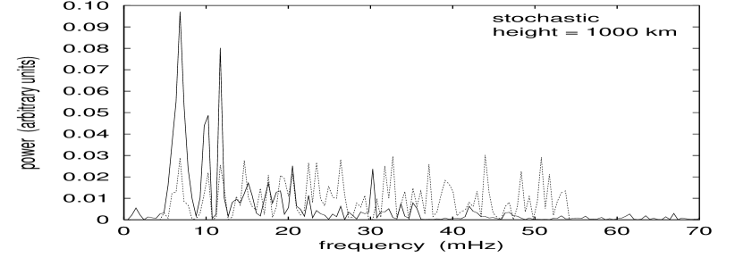


For a comparison with our monochromatic studies we take the same total energy flux erg cm-2 s-1 for the spectra. The initial acoustic wave spectra which excite the solar atmosphere model at height km are shown (dotted) in all panels of Figs. 7 and 8. These figures show (drawn) the acoustic wave spectra at heights , and km (from top to bottom). Furthermore, different timespans for the Fourier analysis are taken. We selected the time intervals 500 - 2548 s (left column) and 2500 - 4548 s (right column). There are two striking results from these spectra. First, it is seen that in both wave cases there is a strong and with height progressing shift of the spectral power from the initially specified one to one which shows a predominant contribution in the 6-8 mHz (3 min) range. Comparing Figs. 7 and 8 it is seen that despite the very different initial shapes of the two spectral cases, they become increasingly similar for greater height. At 2000 km, one has almost pure 3 min spectra in both cases.
The second striking feature of Figs. 7 and 8 is that the spectra at a given height apparently do not vary with time. Comparing the spectra computed from the time interval 500 - 2548 s with those of 2500 - 4548 s at a given height shows that there is essentially no change. This is very different from the monochromatic adiabatic results where the resonance oscillations are transient and die out with time.


As found in our monochromatic studies above, a combination of two conditions will lead to a continuous presence of resonance oscillations: the atmosphere must reach a dynamical equilibrium and the shock merging events must go on indefinitely. Both conditions are met in an excitation with frequency spectra. Figure 9 shows the mean temperatures of the atmosphere as function of time for the two wave cases considered. It is seen that like in Fig. 5, a dynamical steady state temperature distribution is established below 1400 km height after 2000 s and somewhat later after 3500 s at greater height. For the second condition, Fig. 10 shows the plots of the shock merging heights of the two wave cases considered. It is seen that for the Gaussian spectrum, shock merging goes on indefinitely with time in the height interval between 1000 km and the computational boundary at 2220 km. For the stochastic wave case, incessant shock merging occurs in the range 600 to 2000 km.
Because shock merging implies the presence of shocks, and because the initial acoustic frequency spectra have relatively small amplitude with no shocks present, it is clear that the shocks have to be generated during the wave propagation. Figure 11 shows for the stochastic case that different to the situation of monochromatic waves, where all shocks form close to 400 km height (see Fig. 2), the shocks in the case of an acoustic spectrum are formed in a wide range between 300 and 1100 km height. Above 1100 km height, the waves are all sawtooth-type shock waves.
3.6 Shock merging and the generation of 3 min oscillations
At this point we want to discuss in more detail the relation between shock merging and the generation of 3 min oscillations. In the work of Lites et al. (1993) as well as Cheng & Yi (1996) it is argued on basis of observations that in the solar atmosphere the 3 min signal is already present in the lower photosphere and that therefore shock merging is not an important process for the generation of 3 min oscillations. We believe that contrary to this view, our present calculations clearly show that shock merging is a powerful method for generating 3 min oscillations.

Our monochromatic calculations indicate that if the wave periods are not too small, the resonance oscillations die out. However, our calculations with acoustic wave spectra show a fundamentally different behaviour. One might think that in an acoustic spectrum (cf. Fig. 2) the individual partial waves simply form a wavetrain of sawtooth waves and thus do not generate low frequency oscillations. However, the stochastic nature of the superposition of partial waves in an acoustic spectrum perpetually leads to large amplitude fluctuations which invariably generate shocks of different wave period and strength. In addition, note that stochastic superpositions lead to perpetual resonances even in the small amplitude case (see Fig. 14 of Paper I).
The propagation of the shocks in an oscillating atmosphere subsequently results in shock merging events which in turn drive the atmospheric oscillations. Thus acoustic wave spectra will invariably lead to perpetual resonance oscillations. As in our assumed input spectra the 3 min signal is absent, these resonance oscillations must have been generated by the atmosphere in response to the wave excitation. As the acoustic spectrum calculations of Musielak et al. (1994) do not show a prominent 3 min contribution at the top of the convection zone, we consequently conclude that the 3 min band present in the Lites et al. observations must have been added later by hydrodynamic effects in the solar atmosphere. This conjecture will be investigated further in the subsequent paper V.
3.7 Acoustic spectra and the dynamic structure of the atmosphere
A very important result found by comparing the two cases of Fig. 9 is that the mean temperature of the atmosphere in a dynamical steady state strongly depends on the initial wave spectrum. This result also applies to the temperature behaviour of Fig. 5 for the unrealistic case of monochromatic waves. We therefore conclude that the structure of stellar chromospheres is intimately determined by the initial acoustic wave spectrum, generated in the convection zone. It thus should be possible to infer the initial wave spectrum by detailed simulations by comparing theoretical spectra (see e.g. Figs. 7 and 8) and observed spectra at various atmospheric heights.
4 Conclusions
From our adiabatic and non-adiabatic wave calculations for a solar atmosphere model, excited at the bottom by large amplitude monochromatic waves as well as by acoustic frequency spectra, employing a realistic mechanical flux of erg cm-2 s-1, we draw the following conclusions:
1. Adiabatic wave calculations, because of the unbalanced heating, invariably lead to chromospheric temperature plateaus with perpetually rising mean temperatures. This time-dependent growth of the mean temperature makes it increasingly difficult for shock merging to occur. The consequence is that the 3 min type resonances, kicked on by the shock merging events, die out and after some time only the monochromatic signal survives.
2. Non-adiabatic calculations, where the radiative cooling by NLTE H- continua as well as by Mg II and H- Ly lines are considered, invariably establish a dynamically generated mean chromospheric temperature distribution, which at heights below 1400 km is established after 2000 s and at greater height after about 3500 s.
3. For excitation by non-adiabatic monochromatic waves, as already noted in Paper II, a critical frequency Hz is found, which separates domains of drastically different resonance behaviour. For frequencies , the atmospheric resonance decays, leaving behind only the monochromatic signal, while for the resonance oscillation persists and is kicked on by shock merging. For wave periods s, the shock merging occurs undiminished in the height range 1400 to 2200 km. Here the resonances appear self-sustaining.
4. Using two different acoustic wave spectra (Gaussian and stochastic) to excite the atmosphere at height km, we found that in non-adiabatic wave calculations, the spectra showed a characteristic shift towards lower frequency such that at height km essentially only a pure 3 min band exists.
5. We also found that at any given height the acoustic spectra, after an initial time of 500 s, did no longer change with time.
6. In the height interval 1000 - 2200 km for the Gaussian and 600 - 2000 km for the stochastic spectrum, shock merging occurs persistently with time. This self-sustaining shock-merging behaviour is responsible for the fact that there is a 3 min resonance band in the acoustic spectra, which becomes increasingly pronounced with atmospheric height.
7. From our calculations we surmise that the 3 min component observed by Lites et al. (1993) in a low lying iron line, which is not found in the acoustic spectrum generated in the convection zone (Musielak et al. 1994), has been added later by the solar atmosphere as response to the propagation of the acoustic wave spectrum.
8. We find that the dynamically generated mean chromospheric temperature structure is strongly dependent on the assumed initial acoustic wave spectrum. This indicates that detailed wave simulations and height–dependent spectral observations will allow to empirically determine the velocity fluctuations in the acoustic wave generation region. This could be an important independent check of existing convection and sound generation simulations.
9. The appreciable atmospheric expansions found in Paper II did not occur in the present simulations because we now use an Eulerian code.
Acknowledgements.
We thank the Deutsche Forschungsgemeinschaft for grant UL 57/22-1 and NATO for grant CRG-910058. This work was also partially supported by the NASA Astrophysics Theory Program (grant number NAG5-3027) to the University of Alabama in Huntsville (P.U., M.C.). We also gratefully acknowledge valuable comments by F.-L. Deubner and S. Steffens on an earlier version of the manuscript.References
- [1] Buchholz B., Hauschildt P.H., Rammacher W., Ulmschneider P., 1994, A&A 285, 987
- [2] Carlsson M., Stein R.F., 1992, ApJ 397, L59
- [3] Carlsson M., Stein R.F., 1994. In: Carlsson M. (ed.) Proc. Oslo Mini-Workshop at Inst. of Theoretical Astrophysics, Chromospheric Dynamics, p. 47
- [4] Cheng Q.-Q., Yi Z., 1996, A&A 313, 971
- [5] Cuntz M., 1987, A&A 188, L5
- [6] Cuntz M., Ulmschneider P., 1988, A&A 193, 119
- [7] Deubner F.-L., Reichling M., Langhanki R., 1988. In: Christensen-Dalsgaard J., Frandsen S. (eds.) IAU Symp. 123, Advances in Helio- and Asteroseismology, p. 439
- [8] Deubner F.-L., 1991. In: Ulmschneider P., Priest E.R., Rosner R. (eds.) Mechanisms of Chromospheric and Coronal Heating. Springer, Berlin, p. 6
- [9] Fleck B., Deubner F.-L., 1989, A&A 224, 245
- [10] Fleck B., Schmitz F., 1991, A&A 250, 235
- [11] Fleck B., Schmitz F., 1993, A&A 273, 671
- [12] Judge P.G., 1990, ApJ 348, 279
- [13] Kalkofen W., Rossi P., Bodo G., Massaglia S., 1994, A&A 284, 976
- [14] Leibacher J.W., Stein R.F., 1981. In: Jordan S. (ed.) The Sun as a Star. NASA SP-450, p. 263
- [15] Lites B.W., Rutten R.J., Kalkofen W., 1993, ApJ 414, 345
- [16] Musielak Z.E., Rosner R., Stein R.F., Ulmschneider P., 1994, ApJ 423, 474
- [17] Rammacher W., Ulmschneider P., 1992, A&A 253, 586
- [18] Rossi P., Kalkofen W., Bodo G., Massaglia S., 1992. In: Giampapa M.S., Bookbinder J.A. (eds.) Proc. Seventh Cambridge Workshop, Cool Stars, Stellar Systems and the Sun. ASP Conf. Series 26, San Francisco, p. 546
- [19] Rutten R.J., 1995. In: Hoeksema J.T., Domingo V., Fleck B., Battrick B. (eds.) Proc. 4th SOHO Workshop. ESA SP-376, p. 151
- [20] Rutten R.J., 1996. In: Strassmeier K.G, Linsky J.L. (eds.) IAU Symp. 176, Stellar Surface Structure. Kluwer, Dordrecht, p. 385
- [21] Rutten R.J., Uitenbroek H., 1991, Solar Physics 134, 15
- [22] Sutmann G., Ulmschneider P., 1995a, A&A 294, 232 (Paper I)
- [23] Sutmann G., Ulmschneider P., 1995b, A&A 294, 241 (Paper II)
- [24] Sutmann G., Musielak Z.E., Ulmschneider P., 1997, A&A (submitted) (Paper III)
- [25] Ulmschneider P., 1990. In: Wallerstein G. (ed.) Proc. Sixth Cambridge Workshop, Cool Stars, Stellar Systems and the Sun. ASP Conf. Series 9, San Francisco, p. 3
- [26] Ulmschneider P., Rammacher W., Gail H.-P., 1992. In: Giampapa M.S., Bookbinder J.A. (eds.) Proc. Seventh Cambridge Workshop, Cool Stars, Stellar Systems, and the Sun. ASP Conf. Series 26, San Francisco, p. 471