Complex Formulation of
Lensing Theory and Applications

Abstract

The elegance and usefulness of a complex formulation of the basic lensing equations is demonstrated with a number of applications. Using standard tools of complex function theory, we present, for instance, a new proof of the fact that the number of images produced by a regular lens is always odd, provided that the source is not located on a caustic. Several differential and integral relations between the mean curvature and the (reduced) shear are also derived. These emerge almost automatically from complex differentiations of the differential of the lens map, together with Stokes’ theorem for complex valued $1$-forms.

I Introduction

Gravitational lensing has become one of the most important fields in present day astronomy. The enormous activity in this area has largely been driven by considerable improvements of observational capabilities. Gravitational lensing has the distinguished feature of being independent of the nature and the physical state of the deflecting mass. It is therefore perfectly suited to study the dark matter in the Universe [1], [2].

One of the issues which has recently attracted a lot of attention is concerned with parameter-free reconstructions of projected mass distributions from weak lensing data. (For a recent review, see [3].) Thanks to new wide-field cameras and imaging with $8m$-class telescopes, the quality of the data is expected to increase rapidly. Initiated by a paper of Kaiser and Squires [4], a considerable amount of theoretical work on various reconstruction methods has recently also been carried out [5], [6]. The main problem consists in the task to make optimal use of limited noisy data in a parameter-free manner, that is, without modeling the lens.

In the present paper we take up some of the theoretical discussions and demonstrate rather systematically that the complex formulation of lensing theory often simplifies things considerably. In particular, a number of equations which are used in mass reconstructions, emerge almost automatically.

In outline, the paper is organized as follows: For reasons of self-consistency, we provide in Section 2 a brief derivation of the basic lensing equations that are used in the remainder of the paper. These are then translated in Section 3 into a complex formulation, where some mathematical tools are recapitulated as well. It will turn out that the reconstruction problem is basically equivalent to the task of solving the so-called Beltrami equation, at least for noncritical lenses. This part of the paper has considerable overlap with [7]. Turning to applications in Section 4, we give – as far as we know – a new proof of the fact that for a regular lens the number of images is always odd, provided that the source is not located on a caustic. The proof uses only standard tools of complex analysis, which are, for instance, familiar from derivations of the theorem of residues. One of these formulas is an explicit expression for the index of a closed curve relative to a given point. Next, we derive several relations between the mean convergence and the (reduced) shear by (repeated) applications of the complex differential operators $\partial/\partial z$ and $\partial/\partial\bar{z}$ to the differential of the lens map. Several other useful relations for lensing reconstructions, involving integrals over bounded domains, are derived at the end of the paper.

The purpose of this article is mainly methodological. We hope that others will take advantage of it, especially in teaching the pleasant field of gravitational lensing.

II Basic Lensing Equations

For the benefit of those readers who have not studied the extensive monograph of Schneider, Ehlers and Falco [1], we start by giving a brief derivation of the basic lensing equations.

The conceptual basis of gravitational lensing theory is extremely simple. This is at the same time one of the main reasons why it is so important for the astronomical study of mass distributions on all scales. For all practical purposes the ray approximation for light propagation is sufficiently exact. In this limit the rays correspond to null geodesics in a given gravitational field $g$, and the evolution of the polarization vector is governed by the law of parallel transport. (These laws can be deduced from Maxwell’s equations [8].) The null rays are orthogonal to the surfaces of constant phase, $\{S=\mbox{const}\}$, where $S$ is subject to the eikonal equation

$$g^{\mu\nu}\,\partial_{\mu}S\,\partial_{\nu}S\,=\,0\,.$$ (1)

For sufficiently strong lenses the wave fronts develop edges and self-intersections. Clearly, an observer behind such folded fronts sees more than a single image. This is the region of what is called strong lensing and occurs astronomically only rarely.

Here we restrict ourselves to almost Newtonian, asymptotically flat situations. Generalizations to the cosmological context are easy and basically amount to interpret all distances in the formulas given below as angular distances. (For details we refer again to [1], hereafter quoted as SEF). The metric is then given by

$$\mbox{\boldmath$g$}\,=\,\left(1+2\,U\right)\,dt^{2}\,-\,\left(1-2\,U\right)\,d\mbox{\boldmath$x$}^{2}\,,$$ (2)

where $U$ is the Newtonian potential. The spatial part of a light ray satisfies Fermat’s principle,

$$\delta\,\int\frac{d\sigma}{\sqrt{g_{00}}}\,=\,0\,,$$ (3)

for variations with fixed end points [8]. Here $d\sigma^{2}$ denotes the spatial part of the metric (2).

All this can be summarized by saying that gravitational lensing theory is just usual ray optics with the refraction index

$$n(\mbox{\boldmath$x$})\,=\,1\,-\,2\,U(\mbox{\boldmath$x$})\,.$$ (4)

In particular, the ray equation holds,

$$\frac{d}{ds}\,\left(n\,\frac{d\mbox{\boldmath$x$}}{ds}\right)\,=\,\mbox{\boldmath$\nabla$}n\,,$$ (5)

where $s$ is the euclidean path length parameter. (Since light deflection is a scattering process, we can from now on forget about non-euclidean geometry.)

In terms of the unit tangent vector $\mbox{\boldmath$e$}=d\mbox{\boldmath$x$}/ds$, eq. (5) can be written in sufficient approximation as

$$\frac{d}{ds}\,\mbox{\boldmath$e$}\,=\,-2\,\mbox{\boldmath$\nabla$}_{\!\perp}U\,,$$ (6)

where $\mbox{\boldmath$\nabla$}_{\!\perp}$ denotes the transverse derivative, $\mbox{\boldmath$\nabla$}_{\!\perp}=\mbox{\boldmath$\nabla$}-(\mbox{\boldmath$e$},\mbox{\boldmath$\nabla$})\mbox{\boldmath$e$}$. This gives for the deflection angle $\hat{\mbox{\boldmath$\alpha$}}=\mbox{\boldmath$e$}_{in}-\mbox{\boldmath$e$}_{fin}$, with initial and final directions $\mbox{\boldmath$e$}_{in}$ and $\mbox{\boldmath$e$}_{fin}$, respectively,

$$\hat{\mbox{\boldmath$\alpha$}}\,=\,2\,\int_{u.p.}\mbox{\boldmath$\nabla$}_{\!\perp}U\,ds\,,$$ (7)

where the integral is taken over the unperturbed path (u.p.). Here, we insert the expression for the Newtonian potential of a mass density $\rho(\mbox{\boldmath$x$})$. In the well-justified approximation where the extension of the lens (for instance a cluster of galaxies) is much smaller than the distances of the observer and the source to the lens, one finds readily (SEF, Chapter 4)

$$\hat{\mbox{\boldmath$\alpha$}}(\mbox{\boldmath$\xi$})\,=\,4\,G\,\int_{\mbox{$I\!\!R$}^{2}}\frac{\mbox{\boldmath$\xi$}-\mbox{\boldmath$\xi$}^{\prime}}{\mid\mbox{\boldmath$\xi$}-\mbox{\boldmath$\xi$}^{\prime}\mid^{2}}\,\Sigma(\mbox{\boldmath$\xi$}^{\prime})\,d^{2}\xi^{\prime}\,,$$ (8)

where $\Sigma(\mbox{\boldmath$\xi$})$ denotes the projected mass density on the lens plane. (For a point mass this reduces to Einstein’s prediction of light deflection.)

Combining this with elementary geometry, we arrive at the lens map for a given $\Sigma(\mbox{\boldmath$\xi$})$. From Fig.1, which summarizes the notation of SEF, we read off the lens equation

$$\mbox{\boldmath$\eta$}\,=\,\frac{D_{s}}{D_{d}}\,\mbox{\boldmath$\xi$}\,-\,D_{ds}\,\hat{\mbox{\boldmath$\alpha$}}(\mbox{\boldmath$\xi$})\,,$$ (9)

which defines a map from the lens plane to the source plane.

It is convenient to write this in dimensionless form. Let $\xi_{0}$ be a length parameter in the lens plane (whose choice will depend on the specific problem), and let $\eta_{0}$ be the corresponding scaled length in the source plane, $\eta_{0}=(D_{s}/D_{d})\xi_{0}$. We set $\mbox{\boldmath$x$}=\mbox{\boldmath$\xi$}/\xi_{0}$, $\mbox{\boldmath$y$}=\mbox{\boldmath$\eta$}/\eta_{0}$ and (following SEF)

$$\kappa(\mbox{\boldmath$x$})\,=\,\frac{\Sigma(\xi_{0}\/\mbox{\boldmath$x$})}{\Sigma_{crit}}\,,\;\;\;\;\mbox{\boldmath$\alpha$}(\mbox{\boldmath$x$})\,=\,\frac{D_{d}\,D_{ds}}{\xi_{0}\/D_{s}}\,\hat{\mbox{\boldmath$\alpha$}}(\xi_{0}\/\mbox{\boldmath$x$})\,,$$ (10)

with

$$\Sigma_{crit}\,=\,\frac{c^{2}}{4\pi\/G}\,\frac{D_{s}}{D_{d}\/D_{ds}}\,.$$

Then eq. (9) reads as follows

$$\mbox{\boldmath$y$}\,=\,\mbox{\boldmath$x$}\,-\,\mbox{\boldmath$\alpha$}(\mbox{\boldmath$x$})\,,$$ (11)

whereby eq. (8) translates to

$$\mbox{\boldmath$\alpha$}(\mbox{\boldmath$x$})\,=\,\frac{1}{\pi}\,\int_{\mbox{$I\!\!R$}^{2}}\frac{\mbox{\boldmath$x$}-\mbox{\boldmath$x$}^{\prime}}{\mid\mbox{\boldmath$x$}-\mbox{\boldmath$x$}^{\prime}\mid^{2}}\,\kappa(\mbox{\boldmath$x$}^{\prime})\,d^{2}x^{\prime}\,.$$ (12)

It is obvious that $\alpha$ is a gradient of a two-dimensional Newtonian potential:

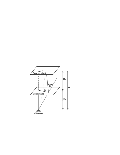
FIG. 1.: Notation adopted for the describtion of the lens geometry.

$$\mbox{\boldmath$\alpha$}\,=\,\mbox{\boldmath$\nabla$}\psi\,,\;\;\;\;\psi\,=\,2\/G\ast\kappa\,,\;\;\;\;G(\mbox{\boldmath$x$})\,=\,\frac{1}{2\pi}\,\ln\mid\mbox{\boldmath$x$}\mid\,\,\,\,\,\,\text{({\hbox{*}} denotes convolution)}\,.$$ (13)

Since $G$ is a fundamental solution of the two-dimensional Laplace operator, $\psi$ satisfies the two-dimensional Poisson equation

$$\Delta\psi\,=\,2\,\kappa\,.$$ (14)

For the differential $D\varphi$ of the map $\varphi\/:\/\mbox{$I\!\!R$}^{2}\rightarrow\mbox{$I\!\!R$}^{2}$, defined by eq. (11), we use the standard parametrization

$$D\varphi\,=\,\left(\begin{array}[]{cc}1-\kappa-\gamma_{1}&-\gamma_{2}\\ -\gamma_{2}&1-\kappa+\gamma_{1}\end{array}\right)\,,$$ (15)

in terms of the mean (Ricci-) curvature $\kappa$, determined by the trace of $D\varphi$, and the (Weyl-) shear vector $\mbox{\boldmath$\gamma$}=(\gamma_{1},\gamma_{2})$. The eigenvalues of the symmetric matrix $D\varphi$ are $1-\kappa\mp\mid\mbox{\boldmath$\gamma$}\mid$. The critical curves, satisfying $\det\left(D\varphi\right)=0$, are given by

$$(1-\kappa)^{2}\,-\,\mid\mbox{\boldmath$\gamma$}\mid^{2}\,=\,0\,.$$ (16)

The caustics are the images of these critical curves. In the vicinity of a caustic the amplification $\mu$, given by

$$\mu\,=\,\frac{1}{\mid\mbox{det}(D\varphi)\mid}\,,$$ (17)

becomes very large.

In passing, we note that the lens map (11) can also be written as

$$\mbox{\boldmath$\nabla$}_{{\mbox{\boldmath$x$}}}\phi\,=\,0\,,\;\;\;\mbox{with}\;\;\phi(\mbox{\boldmath$x$},\mbox{\boldmath$y$})\,=\,\frac{1}{2}(\mbox{\boldmath$x$}-\mbox{\boldmath$y$})^{2}\,-\,\psi(\mbox{\boldmath$x$})\,.$$ (18)

This reflects the Fermat principle. Indeed, the delay of arrival times is directly given by the Fermat potential $\phi$:

$$\triangle t\,=\,\xi_{0}^{2}\,\frac{D_{s}}{D_{d}\/D_{ds}}\,\phi(\mbox{\boldmath$x$},\mbox{\boldmath$y$})\,.$$ (19)

Examples of various lens maps are discussed extensively in Chapter 8 of SEF. Two standard cases are (with suitable choices of $\xi_{0}$):

$$\mbox{Schwarzschild lens:}\;\;\mbox{\boldmath$y$}\,=\,\mbox{\boldmath$x$}\,-\mbox{\boldmath$x$}/\!\mid\mbox{\boldmath$x$}\mid^{2}\,;$$ (20)

$$\mbox{singular isothermal lens:}\;\;\mbox{\boldmath$y$}\,=\,\mbox{\boldmath$x$}\,-\mbox{\boldmath$x$}/\!\mid\mbox{\boldmath$x$}\mid\,.$$ (21)

It is worth recalling the following general fact: In 1955, in a pioneering work of modern singularity theory, H. Whitney [9] studied generic properties of smooth mappings of the plane into itself and proved that the subset of mappings which have only fold and cusp singularities contains an open and dense set (with respect to the Whitney topology). Moreover, those maps of this set which satisfy a few mild global conditions are also stable. Clearly, these results are highly relevant to gravitational lensing. For realistic lenses we will only have folds and cusps, and no singularities of higher order.

III Complex Formulation

In this section we translate the basic lensing equations into a complex formulation. It will turn out that this is not only elegant, but also quite useful, because one can then apply various tools and techniques of complex analysis. This has also been noted before by other authors [7].

A Mathematical Preliminaries

We use standard notation when identifying $\mbox{$I\!\!R$}^{2}$ with $I\!\!\!\!C$, by writing $z=x+iy$ for $(x,y)\in\mbox{$I\!\!R$}^{2}$ and $dz=dx+i\/dy$, $d\bar{z}=dx-i\/dy$ for the corresponding basis of $1$-forms. In terms of the Wirtinger derivatives,

$$\partial_{z}\,\equiv\frac{\partial}{\partial z}\,=\,\frac{1}{2}\left(\frac{\partial}{\partial x}\,-\,i\,\frac{\partial}{\partial y}\right)\,,\;\;\;\;\partial_{\bar{z}}\,\equiv\frac{\partial}{\partial\bar{z}}\,=\,\frac{1}{2}\left(\frac{\partial}{\partial x}\,+\,i\,\frac{\partial}{\partial y}\right)\,,$$ (22)

the differential of any smooth complex function $f$ on $I\!\!\!\!C$ has the representation

$$d\/f\,=\,\frac{\partial f}{\partial z}\,dz\,+\,\frac{\partial f}{\partial\bar{z}}\,d\bar{z}\,.$$ (23)

We shall also write $f_{z}$ and $f_{\bar{z}}$ for $\partial_{z}f$ and $\partial_{\bar{z}}f$, respectively. A function $f$ is holomorphic if and only if $\partial_{\bar{z}}f=0$. In terms of the Wirtinger derivatives the Laplacian is given by

$$\Delta\,=\,4\,\partial_{z}\,\partial_{\bar{z}}\,.$$ (24)

We shall make repeated use of Stokes’ theorem for complex-valued differential forms on $I\!\!\!\!C$ (or an open subset): If $\Omega$ is a compact subset of  $I\!\!\!\!C$ with smooth boundary $\partial\Omega$, then for every complex differential $1$-form $\omega$

$$\int_{\Omega}d\omega\,=\,\int_{\partial\Omega}\omega\,.$$ (25)

An immediate corollary of eq. (25) is the Cauchy-Green formula: For a smooth function $f$ we consider

$$\omega\,=\,f\,\frac{dz}{z-\zeta}\,,$$ (26)

and apply Stokes’ theorem (25) for $\Omega$ minus an $\varepsilon$-disk with center $\zeta$. In the limit $\varepsilon\rightarrow 0$ we obtain

$$f(\zeta)\,=\,\frac{1}{2\pi\/i}\,\int_{\partial\Omega}\frac{f(z)}{z-\zeta}\,dz\,+\,\frac{1}{2\pi\/i}\,\int_{\Omega}\frac{f_{\bar{z}}(z)}{z-\zeta}\,dz\wedge d\bar{z}\,.$$ (27)

For holomorphic functions the second integral is absent. (Note that $dz\wedge d\bar{z}=-2idx\wedge dy$.)

The dilatation or Beltrami coefficient $\nu=\nu_{f}$ of a smooth function $f$ is defined by

$$f_{\bar{z}}\,=\,\nu_{f}\,f_{z}\,,$$ (28)

and this equation is also called Beltrami equation. Since the Jacobian $J_{f}$ of $f$ is given by

$$J_{f}\,=\,\mid f_{z}\mid^{\,2}\,-\,\mid f_{\bar{z}}\mid^{\,2}\,,$$ (29)

we conclude that $\mid\!\nu_{f}\!\mid<1$ if $f$ preserves orientation and $\nu_{f}=0$ if and only if $f$ is conformal. For the interpretation of $\nu_{f}$ we consider the infinitesimal ellipse field by assigning to each $z\in\mbox{$I\!\!\!\!C$}$ the ellipse that is mapped to a circle by $f$. As indicated in Fig. 2, the argument of the major axis of this infinitesimal ellipse is $\left[\pi+arg(\nu_{f})\right]/2$, and the eccentricity $\epsilon$ is

$$\epsilon=\frac{|f_{z}|-|f_{\bar{z}}|}{|f_{z}|+|f_{\bar{z}}|}=\frac{1-|\nu_{f}|}{1+|\nu_{f}|}\,.$$ (30)

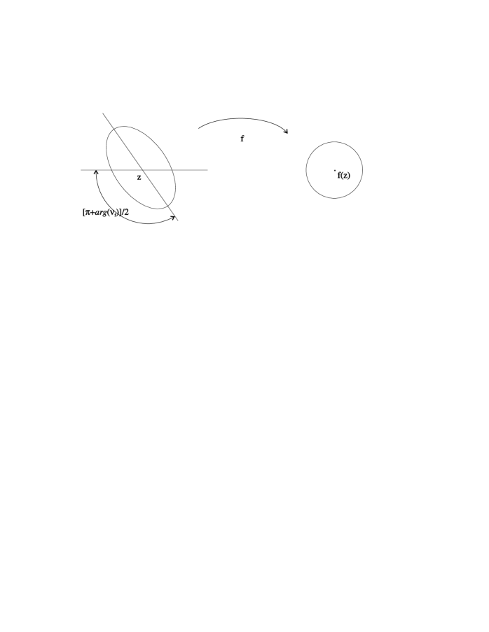
FIG. 2.: Geometrical interpretation of the Beltrami parameter.

Solving the Beltrami equation (28) is then equivalent to finding a function $f$ whose associated ellipse field coincides with a prescribed $\nu$. We shall see that this is just the inversion problem in gravitational lensing. Weak gravitational lensing corresponds to quasiconformal maps. A smooth map $f$ is k-conformal if its Beltrami parameter $\nu_{f}$ satisfies $|\nu_{f}|\leq k<1$. This means geometrically that there is a fixed bound on the stretching of $f$ in any given direction compared to any other direction.

We now quote an existence and uniqueness theorem for the Beltrami equation. For a fixed $k$ with $0<k<1$ let $L^{\infty}(k,\,R)$ denote the measurable functions on $I\!\!\!\!C$ bounded by $k$ and supported in $\left\{z\in\mbox{$I\!\!\!\!C$}|\,|z|<R\right\}$.

Theorem: For $\nu\in L^{\infty}(z,\,R)$, there is a complex function $f$ on $I\!\!\!\!C$, normalized so that $f(z)=z+{\cal O}(1/z)$ at $\infty$, with distributional derivatives satisfying the Beltrami equation $f_{\bar{z}}\,=\,\nu\,f_{z}$, and such that $f_{\bar{z}}$ and $f_{z}-1$ belong to $L^{p}$ for a $p>2$ sufficiently close to 2. Any such $f$ is unique. The solution $f$ is a homeomorphism of $I\!\!\!\!C$, which is holomorphic on any open set on which $\nu=0$. If $\nu\in C^{1}$ and $\nu_{z}\in C^{1}$, then $f\in C^{1}$.

A proof of this theorem can, for instance, be found in [10].

The reconstruction problem (for noncritical lensing) will lead to the inhomogeneous Cauchy-Riemann equation

$$\partial_{\bar{z}}f=h\,.$$ (31)

In case the smooth function $h$ has compact support, the Cauchy-Green formula (27) provides one solution:

$$f\left(\zeta\right)=\frac{1}{2\pi i}\int_{\,\,\mbox{$I\!\!\!\!C$}}\frac{h\left(z\right)}{z-\zeta}dz\wedge d\bar{z}\,.$$ (32)

Obviously, $f$ is only determined up to an additive holomorphic function. If the solution is assumed to be bounded, $f$ is unique up to an additive constant.

From the solution (32) we see that $(\pi z)^{-1}$ is a fundamental solution of the differential operator $\partial_{\bar{z}}$,

$$\frac{1}{\pi}\partial_{\bar{z}}\left(\frac{1}{z}\right)=\delta\,,$$ (33)

because (32) can be written as

$$f=\frac{1}{\pi}\frac{1}{z}*h\,.$$ (34)

A special case of the so-called Dolbaut Lemma in several complex variables implies that one may drop the assumption that $h$ has compact support:

Theorem: For any smooth function $h$ on $I\!\!\!\!C$ there exists a smooth function $f$ such that (31) holds.

For a complete proof, see Chapter 2 of [11].

As an easy consequence we have the

Corollary: For any smooth function $h$ there exists a smooth solution of the Poisson equation $\Delta f=h$.

In the following we often use the abreviations $\partial\equiv\partial_{z}$, $\bar{\partial}\equiv\partial_{\bar{z}}$.

B The complex Lens Mapping and its Differential

The lens mapping $\varphi:\mbox{$I\!\!R$}^{2}\longmapsto\mbox{$I\!\!R$}^{2}$,

$$\mbox{\boldmath$y$}=\varphi\left(\mbox{\boldmath$x$}\right)=\mbox{\boldmath$x$}-\mbox{\boldmath$\nabla$}\psi\left(\mbox{\boldmath$x$}\right)\,,$$ (35)

is now written as $f:\mbox{$I\!\!\!\!C$}\longmapsto\mbox{$I\!\!\!\!C$}$, $w=f(z)$ with $z=x_{1}+ix_{2}$, $w=y_{1}+iy_{2}$. We have

$$f\left(z\right)=z-2\bar{\partial}\psi$$ (36)

or

$$f=\bar{\partial}\left(z\bar{z}-2\psi\right)\,.$$ (37)

Eq. (14) becomes

$$2\partial\bar{\partial}\psi=\kappa\,.$$ (38)

The differential of $f$ will be very important. From (36) and (38) we obtain

$$df=(1-\kappa)dz-2\bar{\partial}^{2}\psi d\bar{z}\,.$$

But

$$\bar{\partial}^{2}\psi=\frac{1}{4}\left(\partial_{1}^{2}-\partial_{2}^{2}\right)\psi+\frac{i}{2}\partial_{1}\partial_{2}\psi=\frac{1}{2}\left(\gamma_{1}+i\gamma_{2}\right),$$

according to the original definition (15) of the shear vector. Introducing the complex shear

$$\gamma=\gamma_{1}+i\gamma_{2}$$ (39)

we obtain

$$df=(1-\kappa)dz-\gamma d\bar{z}\,.$$ (40)

Hence, the Beltrami parameter $\nu_{f}$ of the lens map is given by

$$\nu_{f}=\frac{\gamma}{1-\kappa}\,.$$ (41)

This agrees with the reduced shear introduced by Schneider and Seitz [12].

The examples (20) and (21) become:

$$\text{Schwarzschild lens:}\,f(z)=z-\frac{1}{\bar{z}},\,\nu_{f}=\frac{1}{|z|^{2}}\,;$$ (42)

$$\text{singular isothermal lens:}\,f(z)=z-\frac{z}{|\bar{z}|},\,\nu_{f}=\frac{z}{\bar{z}|z|}\,.$$ (43)

For reference, we note that the amplification $\mu$ is according to (17), (29) and (40) given by

$$\mu^{-1}=|J_{f}|=||\partial f|^{2}-|\bar{\partial}f|^{2}|=|(1-\kappa)^{2}-|\gamma|^{2}|\,.$$ (44)

IV Applications

The usefulness of the complex formulation will be illustrated in this section with several applications. No new results are obtained, but some of the derivations become simpler and more natural.

A Number of Images for a regular Lens

The important fact that the number of images for a regular lens is always odd, provided the source does not lie on a caustic, is traditionally proven with the help of some elements of Morse theory [1]. We now give a proof which uses only standard tools of complex function theory that are used, for example, in the derivation of the theorem of residues. In particular, we make use of the following analytic formula for the index of a closed (rectifiable) curve $\gamma$ relative to a point $a\not\in\gamma$:

$$ind_{\gamma}\left(a\right)=\frac{1}{2\pi i}\int_{\gamma}\frac{dz}{z-a}\,.$$ (45)

This index is equal to the winding number of $\gamma$ around $a$ and hence an integer. Furthermore, it is a homotopic invariant, changes sign under orientation reversion, and is additive under composition of closed curves (see, e.g., Chapter IV of [13]).

Consider now a point $w_{\circ}$ in the source plane with images $f^{-1}\left(w_{\circ}\right)=\left\{z_{1},\dots,\,z_{N}\right\}$ in the lens plane. The complex 1-form

$$\omega=\frac{1}{2\pi i}\frac{df}{f-w_{\circ}}$$ (46)

is regular on $\mbox{$I\!\!\!\!C$}\backslash\bigcup_{j}D_{\epsilon}\left(z_{j}\right)$, where $D_{\epsilon}\left(a\right)$ denotes the closed disk with center $a$ and radius $\epsilon$. It is also closed, and therefore Stokes’ theorem (25) gives

$$\frac{1}{2\pi i}\int_{\partial D_{R}\left(0\right)}\frac{df}{f-w_{\circ}}=\sum_{j=1}^{N}\frac{1}{2\pi i}\int_{\partial D_{\epsilon}\left(z_{j}\right)}\frac{df}{f-w_{\circ}}\,.$$ (47)

Now, for a closed curve $\gamma$ we have by the transformation formula of integrals and (45)

$$\frac{1}{2\pi i}\int_{\gamma}\frac{df}{f-w_{\circ}}=\frac{1}{2\pi i}\int_{f\circ\gamma}\frac{dw}{w-w_{\circ}}=ind_{f\circ\gamma}\left(w_{\circ}\right)\,.$$ (48)

Asymptotically the lens map approaches the identity, and hence the left hand side of (47) is equal to $1$ for $R$ sufficiently large. Therefore, we have

$$1=\sum_{j=1}^{N}ind_{f\circ\partial D_{\epsilon}\left(z_{j}\right)}\left(w_{\circ}\right)=n_{1}-n_{-1}+2\left(n_{2}-n_{-2}\right)+\dots,$$ (49)

where $n_{\lambda}$ denotes the number of $z_{j}$ in $\left\{z_{1},\dots,\,z_{N}\right\}$ for which the index in (49) is equal to $\lambda$.

For the special case, when $w_{\circ}$ is not on a caustic, the Jacobians $J_{f}(z_{j})$ do not vanish and all indices are thus equal to $\pm 1$ ($+1$ if $f$ is orientation preserving and $-1$ if it is orientation reversing at $z_{j}$). Hence

$$N=n_{1}+n_{-1}\,,\,\,\,1=n_{1}-n_{-1}\,,$$ (50)

implying that

$$N=1+2n_{-1}$$ (51)

is odd.

B Relations between mean Convergence and reduced Shear

The Beltrami parameter (reduced shear) $\nu_{f}$ of a lens map is in principle observable. What we are really interested in is, however, the mean curvature $\kappa$ which is related to the surface mass density by (10).

In view of (39) it is natural to look first for relations between the complex shear $\gamma$ and $\kappa$.

Eq. (40) for the differential of the complex lens map and (36) give

$$\gamma=-\bar{\partial}f=2\bar{\partial}^{2}\psi\,.$$ (52)

In order to get a useful relation we differentiate (52) and use (38)

$$\partial\gamma=2\bar{\partial}\left(\partial\bar{\partial}\psi\right)=\bar{\partial}\kappa\,.$$ (53)

This can be regarded as an inhomogeneous Cauchy-Riemann equation for $\kappa$. With the results in Section 3.1 we conclude

$$\kappa=\frac{1}{\pi}\left(\frac{1}{z}\right)*\partial_{\gamma}+\kappa_{\circ}=\frac{1}{\pi}\partial\left(\frac{1}{z}\right)*\gamma+\kappa_{\circ}$$

or

$$\kappa=-\frac{1}{\pi}\frac{1}{z^{2}}*\gamma+\kappa_{\circ}\,.$$ (54)

The additive constant $\kappa_{\circ}$ reflects the fact that a homogeneous mass sheet does not produce any shear (‘mass sheet degeneracy’). The real form of (54) appears the first time in [4]. In making use of (41), we obtain an integral equation for $\kappa$ when $\nu$ is known:

$$\kappa=-\frac{1}{\pi}\frac{1}{z^{2}}*\left[\nu\left(1-\kappa\right)\right]+\kappa_{\circ}\,.$$ (55)

This has been used, for instance, in [6] for nonlinear cluster inversions.

We add that (54) has an inverse, that also appeared in the influencial paper [4] of Kaiser and Squires. From (52) and (13) we obtain

$$\gamma=4\bar{\partial}^{2}G*\kappa\,.$$ (56)

Since the fundamental solution $G$ of the two-dimensional Laplace operator is

$$G=\frac{1}{2\pi}\ln|z|=\frac{1}{4\pi}\ln\left(z\bar{z}\right)$$ (57)

we find

$$\gamma=-\frac{1}{\pi}\frac{1}{z^{2}}*\kappa\,.$$ (58)

Note that (53) has the real form ($\kappa$ is real)

$$\nabla\kappa=\left(\begin{array}[]{c}\partial_{1}\gamma_{1}+\partial_{2}\gamma_{2}\\ \partial_{1}\gamma_{2}+\partial_{2}\gamma_{1}\end{array}\right)\,.$$ (59)

Let us differentiate (53) once more

$$\partial\bar{\partial}\kappa=\partial^{2}\gamma\,,$$ (60)

giving

$$\Delta\kappa=4\partial^{2}\left[\nu(1-\kappa)\right]\,,$$ (61)

from where we could again arrive at (55). The mass-sheet degeneracy is reflected in the following invariance property: Eq. (61), for given $\nu$, remains invariant under the substitution

$$\kappa\longrightarrow\lambda\kappa+(1-\lambda)\,,$$ (62)

where $\lambda$ is a real constant [14].

We can use (53) in a different manner. First, we write this equation as

$$\bar{\partial}\kappa=\partial\left[\nu(1-\kappa)\right]=(1-\kappa)\partial\nu-\nu\partial\kappa\,.$$

This becomes simpler in terms of $K:=\ln(1-\kappa)$:

$$\bar{\partial}K-\nu\partial K=\partial\nu\,.$$ (63)

To this we add its complex conjugate. Noting that $K$ is real, we obtain again an inhomogeneous Cauchy-Riemann equation, this time for $K$:

$$\bar{\partial}K=h(\nu)\,,$$ (64)

whereby the inhomogeneity

$$h(\nu)=(1-|\nu|^{2})^{-1}\left[\partial\nu+\overline{\nu\partial\nu}\right]$$ (65)

is in principal observable.

The real form of this equation was obtained by Kaiser [15] and has often been used in the analysis of cluster data. The complex version appears also in [7].

It should have become clear at this point that the complex formulation is also useful. The relations, derived in this subsection, emerge alsmost automatically by just applying $\partial$ and $\bar{\partial}$ to the coefficients of the differential of the lens map.

C Other useful Reconstruction Equations

Real lensing data are always confined to a finite field of the sky. Therefore, the solution of (64) in the form (32), for example, involving an integration over all of $I\!\!\!\!C$, is in practice not very useful. One can, however, also obtain integral formulas in which only integrations over bounded domains occur.

In order to arrive at these, we write the inhomogeneous Cauchy-Riemann equation in terms of differential forms:

$$d^{\prime\prime}g=\omega\,.$$ (66)

Here $\omega$ is a $1-$form and we use the standard decomposition $d=d^{\prime}+d^{\prime\prime}$ of the exterior derivative, satisfying

$$d^{\prime}\circ d^{\prime}=0\,,\,\,\,d^{\prime\prime}\circ d^{\prime\prime}=0\,,\,\,\,d^{\prime}\circ d^{\prime\prime}+d^{\prime\prime}\circ d^{\prime}=0$$ (67)

(see, e.g., [11]). We make also use of the $\star$-operator, which is related to complex conjugations as follows: If a $1-$form $\alpha$ is decomposed as $\alpha=\alpha_{1}+\alpha_{2}$, where $\alpha_{1}$ is of type $(1,\,0)$ and $\alpha_{2}$ of type $(0,\,1)$, then

$$\star\alpha=i(\bar{\alpha}_{1}-\bar{\alpha}_{2})\,.$$ (68)

The following identities are useful:

$$\star\star\alpha=-\alpha\,,\,\,\,\overline{\star\alpha}=\star\bar{\alpha}\,,$$

$$d\star\left(\alpha_{1}+\alpha_{2}\right)=id^{\prime}\bar{\alpha}_{1}-id^{\prime\prime}\bar{\alpha}_{2}\,,$$

$$\star d^{\prime}g=id^{\prime\prime}\bar{g}\,,\,\,\,\star d^{\prime\prime}g=-id^{\prime}\bar{g}\,,$$

$$d\star dg=2id^{\prime}d^{\prime\prime}\bar{g}=\Delta gdx\wedge dy\,,$$ (69)

where $g$ is a function.

Let now $\Omega\subset\mbox{$I\!\!\!\!C$}$ be a bounded domain with smooth boundary $\partial\Omega$ and $A=|\Omega|$. We show that $g$ minus its average $\bar{g}$ over $\Omega$,

$$\bar{g}=\frac{1}{A}\int_{\Omega}gdx\wedge dy$$ (70)

can be represented in the following form

$$g-\bar{g}=\int_{\Omega}\star\alpha\wedge\omega\,.$$ (71)

The $1-$form $\alpha$ in the integral is given by

$$\alpha=2d^{\prime\prime}H$$ (72)

in terms of the real Green’s function $H$, defined by

$$\Delta H-\frac{1}{A}=-\delta\,,$$ (73)

together with the Neumann boundary condition on $\partial\Omega$.

This is a consequence of Stokes’ theorem. The integrand in (71) is

$$\star\alpha\wedge\omega=\star\alpha\wedge d^{\prime\prime}g=-d^{\prime\prime}\left(g\star\alpha\right)+2fd^{\prime\prime}\left(\star d^{\prime\prime}H\right)\,.$$

By making use of (69) we obtain for the last term

$$gd^{\prime\prime}\left(\star d^{\prime\prime}H\right)=2igd^{\prime\prime}d^{\prime}H=-g\Delta Hdx\wedge dy\,,$$

while the first term is given by

$$-d^{\prime\prime}\left(g\star d^{\prime\prime}H\right)=-d\left(g\star d^{\prime\prime}H\right)\,.$$

Hence,

$$\int\star\alpha\wedge\omega=-\int_{\partial\Omega}g\star d^{\prime\prime}H+g-\bar{g}\,.$$

This is just (71) since the last integral vanishes, due to the Neumann boundary condition for $H$. Formulas equivalent to (71) have been much used by S. Seitz and P. Schneider [6].

The starting point for the derivation of another useful relation is (38) in the form

$$d\left(f-z\right)=-\kappa dz-\gamma d\bar{z}\,,$$

If we wedge this with $d\bar{z}$ and add the complex conjugate of the resulting equation we find

$$\kappa dz\wedge d\bar{z}=\frac{1}{2}d\left[\kappa\left(zd\bar{z}-\bar{z}dz\right)+\gamma\bar{z}d\bar{z}-\bar{\gamma}zdz\right]\,.$$ (74)

Taking the average according to (70) we arrive at

$$\bar{\kappa}=\left\langle\kappa\right\rangle+\frac{\oint\left(\gamma\bar{z}d\bar{z}-\bar{\gamma}zdz\right)}{\oint\left(zd\bar{z}-\bar{z}dz\right)}\,,$$ (75)

where $\left\langle\cdot\right\rangle$ denotes the average along the boundary $\partial\Omega$:

$$\left\langle\kappa\right\rangle=\frac{\oint\kappa\left(zd\bar{z}-\bar{z}dz\right)}{\oint\left(zd\bar{z}-\bar{z}dz\right)}\,.$$ (76)

For the special case of a disk $D_{r}$ we have along the boundary $z=re^{i\varphi}$, $zd\bar{z}-\bar{z}dz=-2ir^{2}d\varphi$, hence

$$\bar{\kappa}=\left\langle\kappa\right\rangle+\left\langle\gamma_{t}\right\rangle\,,$$ (77)

where $\gamma_{t}$ denotes the tangential component of the shear

$$\gamma_{t}=\gamma_{1}\cos 2\varphi+\gamma_{2}\sin 2\varphi\,.$$ (78)

This relation is not new (see Ref. [5]). Noting that

$$\bar{\kappa}=\frac{1}{\pi r^{2}}\int_{0}^{r}\kappa\left(r^{\prime},\,\varphi\right)r^{\prime}dr^{\prime}d\varphi\,,$$ (79)

and thus

$$\frac{d\bar{\kappa}}{d\ln r}=2\left\langle\kappa\right\rangle-2\bar{\kappa}\,,$$ (80)

we can use (77) to obtain the interesting connection

$$\frac{d\bar{\kappa}}{d\ln r}=-2\left\langle\gamma_{t}\right\rangle\,.$$ (81)

This has recently been used in an analysis of weak lensing data [5]. A useful integral form of it is, in obvious notation,

$$\bar{\kappa}\left(r_{1}\right)-\bar{\kappa}\left(r_{1}<r<r_{2}\right)=2\left(1-\frac{r_{1}^{2}}{r_{2}^{2}}\right)^{-1}\int_{r_{1}}^{r_{2}}\left\langle\gamma_{t}\right\rangle\frac{dr}{r}\,.$$ (82)

The left hand side of this equation is what Kaiser and Squires call the $\zeta$-statistics, $\zeta\left(r_{1},\,r_{2}\right)$. One can use general weight functions for the average process [5] and try to optimize the choice for the detection of mass overdensities [6]. Note also, that the integral on the right in (82) can be written as

$$\int_{r_{1}}^{r_{2}}\left\langle\gamma_{t}\right\rangle\frac{dr}{r}=\frac{1}{2\pi}\int_{\left[r_{1},\,r_{2}\right]}\Re\left(\frac{1}{\bar{z}^{2}}\bar{\gamma}\right)dx\wedge dy\,.$$ (83)

We conclude by pointing out another appearance of a Beltrami parameter in lensing theory. An often used method for describing the shape of a galaxy image uses the second brightness moments

$$Q_{ij}=\frac{1}{Norm}\int I\left(\mbox{\boldmath$x$}\right)\left(x_{i}-\bar{x}_{i}\right)\left(x_{j}-\bar{x}_{j}\right)d^{2}x\,,$$ (84)

where $I\left(\mbox{\boldmath$x$}\right)$ is the surface brightness distribution and $\bar{\mbox{\boldmath$x$}}$ is the center of light of the galaxy image. Regard now $Q=\left(Q_{ij}\right)$ as a linear map of $\mbox{$I\!\!R$}^{2}$. If this is interpreted as a map $z\longmapsto w\left(z\right)$ of $I\!\!\!\!C$ it reads

$$w=\frac{1}{2}\left(Q_{11}+Q_{22}\right)z+\frac{1}{2}\left(Q_{11}-Q_{22}+2iQ_{12}\right)\bar{z}=\frac{1}{2}trQ\left[z+\chi\bar{z}\right]\,,$$ (85)

where

$$\chi=\frac{\left(Q_{11}-Q_{22}+2iQ_{12}\right)}{trQ}\,.$$ (86)

$\chi$ is called the complex ellipticity and is clearly just the Beltrami parameter of the map (85). The intrinsic brightness moments $Q_{ij}^{\left(s\right)}$ of the galaxy are defined corespondingly and it is easy to see that $Q^{\left(s\right)}=D\varphi\cdot Q\cdot D\varphi$, $D\varphi$ being the differential (15) of the lens map. The interpretation of $\chi$ just given, allows us to find easily the corresponding relation between $\chi$ and $\chi^{\left(s\right)}$. One just has to compose the map (85) on the right and on the left with the linearized lens map

$$w=\left(1-\kappa\right)z-\gamma\bar{z}\,.$$ (87)

This gives readily

$$\chi^{\left(s\right)}=\frac{-2\nu+\chi+\nu^{2}\bar{\chi}}{1+|\nu|^{2}-2\Re\left(\nu\bar{\chi}\right)}\,,$$ (88)

with the inverse

$$\chi=\frac{2\nu+\chi^{\left(s\right)}+\nu^{2}\bar{\chi}^{\left(s\right)}}{1+|\nu|^{2}+2\Re\left(\nu\bar{\chi}^{\left(s\right)}\right)}\,.$$ (89)

A real derivation of these formulas is quite akward. They are used in applications by averaging over a set of galaxy images, together with statistical assumptions about the intrinsic ellipticity distribution (for instance $\left\langle\chi^{\left(s\right)}\right\rangle=0$), to determine the reduced shear $\nu$ of the lens map. Here, we just wanted to point out that $\chi$ has the interpretation of a Beltrami parameter and that the relations (88) and (89) are very easily obtained in the complex formalism.

We hope that the reader will find other examples of such simplifications.

V Acknowledgments

I thank Philippe Jetzer for interesting conversations and Markus Heusler for a careful reading of the manuscript. Marcus Strässle helped me in shaping the final version.

REFERENCES

- [1] P. Schneider, J. Ehlers, E.E. Falco, Gravitational Lenses, Springer-Verlag (1992).
- [2] P. Schneider, in: Cosmological Applications of Gravitational Lensing, Lecture Notes in Physics, eds. E. Martinez-Gonzlez & J.L. Sanz, Springer-Verlag (1996); P. Schneider, Helv. Phys. Acta, 69, 373 (1996).
- [3] N. Kaiser, Gravitational Lensing, Texas Symposium on Relativistic Astrophysics, Ann. New York Akad. Sci. (1997), to appear.
- [4] N. Kaiser, G. Squires, Astrophys. J. 404, 441 (1993).
- [5] N. Kaiser, G. Squires, T. Broadhurst, Astrophys. J. 449, 460 (1995).
- [6] S. Seitz, P. Schneider, Astron. Astrophys. 305, 383 (1996)
- [7] T. Schramm, R. Kayser, Astron. Astrophys. 299, 1 (1995)
- [8] N. Straumann, General Relativity and Relativistic Astrophysics, Springer- Verlag 1984.
- [9] H. Whitney, Ann. Math., 62, 374, (1955).
- [10] L. Carlson, T.W. Gamelin, Complex Dynamics, Universitext: Tracts in Mathematics, Springer-Verlag (1993).
- [11] O. Forster, Lectures on Riemann Surfaces, Graduate Texts in Mathematics 81, Springer-Verlag (1981).
- [12] P. Schneider, C. Seitz, Astron. Astrophys. 294, 411 (1995).
- [13] J.B. Conway, Functions of One Complex Variable, Graduate Texts in Mathematics 11, Springer-Verlag (1973).
- [14] C. Seitz, P. Schneider, Astron. Astrophys. 297, 287 (1995).
- [15] N. Kaiser, Astrophys. J. 439, L1 (1995).