The Formation and Evolution of Clusters of Galaxies in Different Cosmogonies

Abstract

The formation of galaxy clusters in hierarchically clustering universes is investigated by means of high resolution N-body simulations. The simulations are performed using a newly developed multi-mass scheme which combines a PM code with a high resolution N-body code. Numerical effects due to time stepping and gravitational softening are investigated as well as the influence of the simulation box size and of the assumed boundary conditions. Special emphasis is laid on the formation process and the influence of various cosmological parameters. Cosmogonies with massive neutrinos are also considered. Differences between clusters in the same cosmological model seem to dominate over differences due differing background cosmogony. The cosmological model can alter the time evolution of cluster collapse, but the merging pattern remains fairly similar, e.g. number of mergers and mass ratio of mergers. The gross properties of a halo, such as its size and total angular momentum, also evolve in a similar manner for all cosmogonies and can be described using analytical models. It is shown that the density distribution of a halo shows a characteristic radial dependence which follows a power law with a slope of $\alpha=-1$ at small and $\alpha=-3$ at large radii, independent of the background cosmogony or the considered redshift. The shape of the density profiles follows the generic form proposed by Navarro et al. (1996) for all hierarchically clustering scenarios and retains very little information about the formation process or the cosmological model. Only the central matter concentration of a halo is correlated to the formation time and therefore to the corresponding cosmogony. We emphasise the role of non-radial motions of the halo particles in the evolution of the density profile.

1 Introduction

Clusters of galaxies are the most massive, gravitationally bound objects in the universe. Since their average density is only several hundred times as large as the critical density of the universe and since their collapse time is comparable to the age of the universe, they are likely to have formed recently. Such a recent formation is also implied by substructure observed for many galaxy clusters. It is conceivable that non-linear dynamics and violent relaxation has not yet erased all information about the initial conditions and the formation process itself. Therefore, galaxy clusters may give insight into how structure has grown in the universe. In order to extract these insights from the structure of a galaxy cluster observed at a given epoch, its formation process has to be understood in detail. One important aspect is the connection between the actual structure of dark matter haloes and the features of a given theory of structure formation. The density profile of a dark matter halo at a given epoch may be determined by the initial power spectrum as well as by the present density parameter $\Omega_{0}$ and/or the value of the cosmological constant $\Lambda$.

Such a dependence between the initial power spectrum and the density profiles of virialized objects was pointed out by Hoffman & Shaham (1985) and Hoffman (1988). Their analytic work was based on the assumption of Gaussian random fields with scale free power spectra $P(k)\propto k^{n}$. Based on the secondary infall model of Gunn & Gott (1972), and the self-similar solution of Fillmore & Goldreich (1984) and Bertschinger (1985), they found that the slope of the density profiles becomes steeper with increasing spectral index $n$. Analytic calculations, however, are based on simplifying assumptions (e.g. spherical symmetry) and, therefore, cannot consider all aspects of gravitational collapse. N-body simulations, which begin with generic initial conditions, provide an attractive alternative. Though the effects of gas dynamics are neglected, they are likely to represent a realistic description of the formation of galaxy clusters: observations suggest that dark matter dominates the mass of galaxy clusters and largely determines their gravitational potential. Only in the highest density regions near the center of a cluster are the time scales sufficiently short that the cluster dynamics can be influenced by hydrodynamical effects.

Within the last couple of years, multi-mass techniques have been developed which allow one to investigate the formation of individual clusters with high numerical resolution. Navarro et al. (1996a) (hereafter NFW) have investigated the structure of dark matter haloes which form in a cold dark matter (CDM) universe ($\Omega_{0}=1$). They found that the density profiles of haloes do not follow a power law, but tend to have a slope $\alpha=\frac{d\ln\varrho}{d\ln r}$ with $\alpha=-1$ near the cluster center and $\alpha=-3$ at large radii. Over more the four orders of magnitude in mass, the density profiles follow a universal law, which can be parameterized by

$$\frac{\varrho(r)}{\varrho_{b}}=\frac{\delta_{n}}{\frac{r}{a_{n}}(1+\frac{r}{a_{n}})^{2}}.$$ (1)

The two free parameter are the scale radius $a_{n}$ which defines the scale where the profile shape changes from $\alpha>-2$ to $\alpha<-2$ and the characteristic overdensity $\delta_{n}$. Equation (1) differs in its asymptotic behaviour at large radii from the profile

$$\frac{\varrho(r)}{\varrho_{b}}=\frac{\delta_{h}}{\frac{r}{a_{h}}(1+\frac{r}{a_{h}})^{3}}.$$ (2)

which was proposed by Hernquist (1990) to describe the mass profiles of elliptical galaxies. This profile has also been used by Dubinsky & Carlberg (1991) to fit the density distribution of haloes which were formed in their CDM-type simulation. Lacey & Cole (1996) extended the work of NFW to scale free power spectra with $n=-2,-1$, and 0 in an $\Omega_{0}=1$ cosmogony, though with a lower numerical resolution. Tormen et al. (1996) have done simulations with an $n=-1$ scale free power spectrum and $\Omega=1$ and with an even higher numerical resolution than NFW. Recently, Navarro, Frenk and White (1996b) extended their study to cosmogonies with $\Omega<1$ and with a non-vanishing cosmological constant $\Lambda$. Haloes which form in all of these cosmological models seem to be well described by equation (1). The scale radius and the central overdensity seem to be related to the formation time of the halo (Navarro et al.  1996b). These results suggest that the density profile found by NFW is quite generic for any scenario in which structures form due to hierarchical clustering. The power spectrum and cosmological parameters may only indirectly enter by specifying the typical formation epoch of a halo of a given mass. Consequently, they possibly affect the profiles of galaxy clusters only by specifying the dependence of the characteristic radius $a$ on the total mass of a cluster.

In this paper we concentrate on the profiles of galaxy clusters and investigate the influence of the background cosmogony. Models with $\Omega<1$ and/or $\Lambda\neq 0$ are considered as well as scenarios with a cold and a hot component. Also a pure hot dark matter model is considered as an example of a cosmogony in which structure does not form hierarchically. We investigate the formation history of haloes and its dependence on the background cosmogony. We also present results for other gross properties such as the triaxiality and angular momentum of the haloes. Their evolution is compared with the analytical predictions of the spherical top-hat model. The structure of the paper is as follows. In section 2 we present the different considered cosmogonies and briefly describe their impact on structure formation. Section 3 presents the numerical techniques and discusses the issues of numerical resolution, time stepping and boundary conditions. Section 4 investigates the collapse of individual haloes in detail showing the evolution of various halo properties. The structure of the haloes and their dependence on the background cosmogony is analysed in section 5. We summarise our results and conclude in Section 6.

2 The cosmological models

Seven cosmological models are studied in this paper. Three of these are cold dark matter models (CDM, OCDM and LCDM) representing flat, open and $\Lambda$ dominated cosmologies. The three mixed dark matter models (CHDM I-III) contain differing number and masses of neutrino species. These models thus cover a broad range of hierarchical structure formation scenarios. The HDM model is added to investigate the formation of clusters in a cosmogony which does not follow the hierarchical scenario. Table 1 gives the cosmological parameters defining the seven different cosmological models.

It is far from obvious what is the best way to compare galaxy clusters as they form in different cosmological scenarios. Potential choices involve comparing clusters of similar mass or similar $M/M_{*}$, among others. The nonlinear mass $M_{*}$ is defined as the mass corresponding to the linear rms density fluctuation which exceeds the critical threshold $\delta_{c}(z)$ for collapse at a given redshift in the spherical top-hat model (Eke et al.  1996). Values for $M_{*}$ at $z=0$ are given in table 2. All these criteria yield a different set of objects which are compared. The problems are further complicated by some freedom in the choice of the normalisation of the power spectrum (e.g. COBE normalised versus normalised according to cluster abundance). Finally, high resolution cluster simulations are still computationally expensive, and a numerical study is restricted to a few objects per cosmological scenario. Differences in the formation history due to different realisations of a Gaussian random field can be larger than those induced by the features of a individual cosmogony. In order to minimise these sampling effects, we use identical phases for the Gaussian random field for each of the three considered realisations. Each realisation corresponds to one massive cluster at $z=0$. In the following we will refer to the realisations as realisation A, B and C. For the HDM model, 2 simulations have been performed, corresponding to realisations A and C.

We normalise all power spectra to $\sigma_{8}=0.63$, i.e. all models have the same linear extrapolated rms overdensity in top-hat spheres of radius $8/h\,$Mpc. This normalisation reproduces the observed abundance of rich galaxy clusters (White et al.  1993) in the case of a high $\Omega$ universe, but is low for the LCDM and OCDM models. Recent results of Eke et al.  (1996) suggest $\sigma_{8}=0.5\;\Omega_{0}^{-0.52}$ ($\sigma_{8}=0.5\;\Omega_{0}^{-0.46}$) for the LCDM (OCDM). Thus $\sigma_{8}=0.97$ ($\sigma_{8}=0.9$) for $\Omega=0.3$, which is larger than our choice by a factor of $1.5$ ($1.4$). Similar results also hold for COBE normalisation. While the standard CDM scenario is inconsistent with the COBE measurements, the CHDM sequences fit both COBE measurements and cluster abundances. A disadvantage of our normalisation is that clusters in different cosmological models have different masses and circular velocitys as shown in figure 1. The models with $\Omega<1$ have approximately a mass smaller by a factor of $\Omega$ and a circular velocity smaller by $\Omega^{1/3}$ than the $\Omega=1$ CDM models. Since $M_{*}$ is smaller by a similar amount, they have a similar $M/M_{*}$ as the CDM clusters, i.e. they are similarly rare events at $z=0$. The clusters of the CHDM models have a much higher $M/M_{*}$ and are, therefore, much rarer events.

The simulations are done in a periodic cubic box with a side length of $250\;h^{-1}\,$Mpc. The mass resolution is $2.5\times 10^{11}\;h^{-1}\Omega\;\mbox{M${}_{\odot}$}$. Therefore, a cluster with a mass of $10^{15}\;h^{-1}\Omega\;{\mathrm{M}_{\odot}}$ consists of 4000 particles. The spatial resolution set by the force softening and time stepping is $12.5\;h^{-1}\,$kpc. All simulations are started at a redshift of $z=19$ and end at the present time. After every increase of $0.05$ in the expansion factor an output of position, velocity, potential and force of the particles is stored, leading to a total of 20 outputs per simulation.

The initial conditions for the CDM and CHDM runs were generated using the COSMIC code by Bertschinger et al.  (1995). For the LCDM cosmogony the power spectrum given by Efstathiou et al.  (1992) is used while the OCDM and HDM cosmogonies are based on those given by Bardeen et al.  (1986).

Figure 1: Mass and circular velocity for the simulated cluster models. Circles correspond to clusters formed in OCDM models, stars to LCDM, plus signs to CDM, triangles to CHDM I, diamonds to CHDM II, squares to CHDM III and crosses to HDM.

Table 1: The cosmological parameters of the models. The columns give the name of the model, the present density parameter of the cold and hot component of matter, and the density parameter associated with the cosmological constant $\Omega_{\Lambda}=\frac{\Lambda}{3H_{0}}$, the Hubble parameter h, and the number of massive neutrinos.

Model	$\Omega_{\mathrm{cold,0}}$	$\Omega_{\mathrm{hot,0}}$	$\Omega_{\Lambda}$	$h$	$N_{\nu}$
CDM	1.0	0	0	0.5
LCDM	0.3	0	0.7	0.7
OCDM	0.3	0	0	0.7
CHDM I	0.8	0.2	0	0.5	3
CHDM II	0.8	0.2	0	0.5	1
CHDM III	0.7	0.3	0	0.5	1
HDM I	0	1.0	0	0.5	1

Table 2: The effective slope of the power spectrum at $k=0.2\;h\;{\mathrm{M}pc}^{-1}$ and the nonlinear Mass $M_{*}(z=0)$ of the different power spectra.

Model	$n_{\rm eff}$	$M_{*}/M_{\odot}$
CDM	-1.12	$1.60\times 10^{13}$
LCDM	-1.60	$4.61\times 10^{12}$
OCDM	-1.74	$5.10\times 10^{12}$
CHDM I	-1.64	$2.26\times 10^{12}$
CHDM II	-1.73	$2.16\times 10^{12}$
CHDM III	-2.10	$1.82\times 10^{11}$
HDM	-3.64	not defined

The standard picture of structure formation involves the gravitational collapse of density inhomogeneities in an otherwise uniform universe. A simple analytic description of this process is the spherical top-hat model (Peebles 1980), which assumes a uniform spherical overdensity. The time evolution of a halo with mass $M$ and radius $R$ is given by the Tolman-Bondi equation,

$$\dot{R}^{2}=2GMR^{-1}+\frac{\Lambda}{3}R^{2}-2E,$$ (3)

where $E$ is the total energy of the halo and has to be $<0$ for a collapse. This model gives the mean over-density $\bar{\delta}(z)$ of a region which is required for collapse,

$$1+\bar{\delta}(z) > \frac{1}{\Omega(z)}\qquad\Omega_{\Lambda}=0$$ (4)

$$> 1\qquad\Omega_{0}+\Omega_{\Lambda}=1.$$

In a flat universe any overdense region is able to collapse, whereas in an open universe $\bar{\delta}(z)$ has to be above a critical value. The mean density of an object after virialisation can also be estimated in the spherical collapse model. Using the results of Eke et al.  (1996) the value of this density, hereafter virial density, can be adequately approximated for various cosmological background models by

$$\rho_{\rm vir}(z)=180\;\Omega(z)^{-m}\rho_{b}(z)\,,$$ (5)

where $\Omega(z)$ and $\rho_{b}(z)$ are the density parameter and the background density at redshift $z$. The value of the power index $m$ depends on the presence of a cosmological constant. For $\Lambda=0$ $m=0.66$, while for $\Omega+\Omega_{\Lambda}=1$, $m=0.52$.

The spherical collapse model is, however, a strong simplification for structure formation in hierarchically clustering scenarios. Tracing back collapsed structures to high redshift shows that structures form from highly irregularly shaped volumes (see e.g. figure 7) which also possess a large amount of substructure. The formation of a halo of the size of a cluster must not be only the result of spherical accretion of matter shells but can also be formed by merging of smaller matter accumulations. Generally the evolution pattern is influenced by the overall distribution of the inhomogeneities and the cosmological background model. In the following we will discuss how the cosmological background model and the kind of dark matter affect the formation of a halo.

There is an important difference between the models based on an Einstein-de Sitter universe and the models with $\Omega<1$ concerning the time evolution of the density inhomogeneities. At high redshifts when linear theory is valid the growth of overdensities can be described by $\delta({\bf x},z)=D(z)\delta_{0}({\bf x})$ (Peebles 1980). $\delta({\bf x},z)$ is the local density contrast at redshift $z$, $\delta_{0}({\bf x})$ the linearly extrapolated value at the present time and $D(z)$ the linear growth factor. It gives the growth rate of the overdensities in linear theory. In an EdS universe $D(z)=a=1/(1+z)$. In a universe with $\Omega<1$, the slope of $D(z)$ is shallower for low $z$. Since the growth factor is normalised to $D(0)=1$, $D(z)$ is thus larger at higher redshifts and the nonlinear regime is reached earlier than in the models based on the EdS universe. For $\Omega=0.3$, $D/a\approx 2$ for an open universe ($\Lambda=0$) at a redshift of $z=19$, and $D/a\approx 1.3$ for a flat universe ($\Lambda=1-\Omega$). However in an open universe an overdense region needs a higher density contrast to collapse than in a flat universe due to equation (4). This shifts the beginning of structure formation to smaller $z$-values in an open universe, partially neutralizing the effect of a higher growth factor relative to a flat universe with the same density parameter.

The general distribution of inhomogeneities depends on the shape of the power spectrum $P(k)$, which in turn is set by the density parameter and the physical properties of the assumed dark matter. In figure 2 the power spectra of all cosmogonies used are plotted. On the basis of the asymptotic behavior of the power spectra at high wave numbers one can distinguish between two different structure formation scenario: the hierarchical scenario and the non-hierarchical (top-down) scenario.

Figure 2: Power spectra $P(k)$ of all cosmoginic models are compared at $z=19$: a) $P(k)$ of the CDM (solid), LCDM, (dash triple-dotted) and the OCDM model (long-dashed); b) the total power spectra of the three CHDM models (I: dotted, II: dash dotted, III: dashed) and the HDM model (solid); c) and d) $P(k)$ for the two components of the mixed dark matter models seperatly, c) for the cold and d) for the hot component.

Power spectra with an asymptotic slope larger than $-3$ have more power on small scales. This feature is believed to lead to a hierarchical scenario, where small objects collapse first and large object like clusters form later by merging of smaller ones. All models except for the HDM cosmogony follow this pattern. The detailed evolution pattern in the hierarchical scenario depends on the effective slope $n_{\rm eff}$ of the power spectrum near $k_{\rm cl}$, the wave vector which corresponds to the mass of a considered cluster. For a cluster mass of $10^{15}\;h^{-1}\Omega\;\mbox{M${}_{\odot}$}$ and $\sigma_{8}=0.63$ this is $k_{\rm cl}\approx 0.2\;h\;$Mpc^-1. Since $k_{\rm cl}$ is similar to the wave number at which the power spectra have been normalised, the amplitude of $P(k)$ is similar at $k_{\rm cl}$. The degree of inhomogeneity on small scales is related to the value of $n_{\rm eff}$. Values of $n_{\rm eff}$ are also given in Table 2 for all models. For similar overdensities under equal cosmological conditions small scale structure is more pronounced in cosmogonies with larger values of $n_{\rm eff}$ or equivalently of $M_{*}$. Small scale objects are more numerous and form at earlier redshift, leading to a higher merging rate of these objects than in models with small $n_{\rm eff}$ or $M_{*}$. Within our models the most small scale power is in the CDM and the smallest in the CHDM III simulations. The steeper slope of the OCDM and LCDM models compared to SCDM are almost compensated by the initially faster growth of the fluctuations.

In the mixed dark matter simulations gravitational clustering is more complex due to the mutual interaction between the hot and cold components. Due to free streaming, the hot component is initially much more homogeneously distributed than the cold component. The smaller overall overdensities also suppress the growth of density fluctuations in the cold component which thus proceeds slower than $\propto(1+z)^{-1}$, the linear growth rate for a pure CDM model. Only at low redshifts has the velocity dispersion of massive neutrinos decreased sufficiently due to the expansion of the universe that the neutrinos are able to fall into and virialise within the potential wells formed by the cold dark matter. The details of the power spectrum and the non-linear clustering thus depend on the mass fraction of the hot dark matter as well as on the mass of the neutrinos themselves, i.e. on the number of families of massive neutrinos (for a given mass fraction of hot dark matter). This dependence can be seen in the power spectra of the cold and the hot component (Figure 2 c,d). The suppression of large scale power in the cold component is most pronounced in the CHDM III model due to the high mass fraction in neutrinos ($\Omega_{\rm hot}=0.3$). Suppression of small scale structure is most pronounced for the CHDM I model. It has three families of massive neutrinos and, therefore, the lowest neutrino mass ($m_{\nu}=6h^{2}\,eV$).

In the case of the HDM model the asymptotic slope is less than $-3$. One cannot specify $M_{*}$ since the linear rms density fluctuation for HDM (normalised to $\sigma_{8}=0.63$) never exceeds the critical threshold for spherical collapse. Some peaks however are sufficiently high and exceed $\delta_{c}(z)$. Large scale modes become nonlinear first in HDM simulation, leading to the formation of clusters before galaxy sized objects are present. This should cause the evolution of haloes to be qualitatively very different in the HDM cosmogony. Since there is no small scale power in the initial spectrum, the formation of a halo should be similar to the collapse of an overdense region in the spherical top-hat model. However, this qualitative expectation needs to be checked by examining the evolution of HDM clusters in the simulations.

3 Numerical techniques

It is computationally challenging to perform numerical simulations which allows one to analyse the density distribution of galaxy clusters in sufficient detail. Such simulations must not have a spatial resolution worse than a couple of tens of kpc. In order to include the tidal field exerted by a cosmologically representative sample of the universe, however, simultaneously a box with a side length of several hundreds of Mpc has to be covered. The high spatial resolution also requires a fine grained time stepping which gives rise to a total number of time steps of more than $10^{4}$. In the traditional approach of large scale N-body simulations using (adaptive) P3M (see, e.g. Efstathiou et al.  1985, Couchman 1991), such simulations, if at all possible, require the computing power of state of the art massively parallel supercomputers.

As an alternative to large N-body simulations, multi-mass techniques have been developed (Porter 1985). In analogy to the concept of tree codes, the tidal field of the surrounding matter is represented by particles whose mass increases logarithmically with distance. These techniques have been successfully applied to the formation of galaxies and of galaxy clusters (Katz & White 1993, Navarro, Frenk & White 1995, Bartelmann, Steinmetz & Weiss 1995). Its disadvantage is that only one or a few objects can be studied per simulation, and the selection of the region which potentially forms an object involves some bias.

In this section we describe a new variant of such a multi-mass technique, using nested distributions of particles with different mass. Additional a high resolution N-body integrator is combined with a low resolution particle-mesh (PM) code. Such a hybrid technique combines the advantages of PM and high resolution codes: (i) it naturally provides periodic boundary conditions, (ii) the forces within the high resolution follow a $r^{-2}$ law, smoothed by a plummer or a spline softening and (iii) a smooth sampling of the external force field surrounding the object of interest is given. Two-body relaxation due to accidental encounters of particles which largely differing mass can be suppressed, which may be of even more importance for simulations including the effects of gas dynamics (Steinmetz & White 1996). The periodic extension under preservation of the Newtonian force law is especially interesting for codes which use the special purpose hardware GRAPE (Sugimoto et al.  1989), where a plummer force law is hardwired. But also in the case of tree codes such a feature is of interest. In contrast to the Ewald summation technique (Ewald 1921, Hernquist et al.  1991), it easily and memory efficiently allows one to combine periodic boundary conditions and higher order multipole moments calculating the tree force.

3.1 Initial conditions

The initial particle arrangement consists of a hierarchy of four nested particle distributions (see figure 3, 5). The particle mass increases by a factor of eight going from one hierarchy to the next. The hierarchy with the lowest resolution covers the simulation box with periodic boundary conditions and a side length of $250\;h^{-1}\;$Mpc. A sphere with a radius of $1/16$th of the box size is the highest resolution region. All particles which can be found within the virial radii of galaxy clusters studied in this paper are acquired from this sphere. The highest and lowest resolution regions are connected by two intermediate spherical shells of particles, the outer radius of these shells being $1/8$th and $1/4$th of the box size, respectively. In the central region the dynamic range of the simulation therefore corresponds to a simulation with $256^{3}$ particles per dark matter species, however, the actual particle number is only $\approx 3\times 64^{3}$.

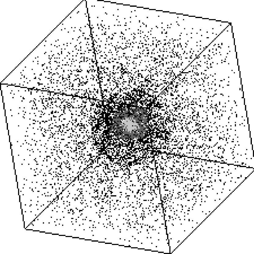
Figure 3: Initial particle configuration showing the hierarchy of four nested particle distributions.

The initial particle distribution within each hierarchy consists of a glass-like particle arrangement, i.e. the force on every individual particle equals zero. Like a Poissonian sample, and in contrast to a grid, such a particle arrangement has no preferred direction, but contrast to a Poissonian sample, it also has no considerable large scale power up to the Nyquist frequency (Efstathiou et al.  1995). It can easily be created assuming repulsive rather than attractive interparticle forces (White 1996). Each level uses the same glass-like particle arrangement but with different mass assigned to the particles.

In the case of models with hot and cold dark matter, each component is represented by a separate particle distribution. The mass of each particle is scaled according to the relative contribution of each component. In order to prevent particles having nearly identical initial positions the distributions for each species is drawn from a different realisation of a glass-like particle arrangement.

To realise a Gaussian random field with a given power spectrum, the position of every particle is perturbed according to the Zel’dovich approximation (Zel’dovich, 1970). For the lower mass hierarchies, the displacement vectors consist of the identical wave numbers as used for the surrounding distributions and of additional wave numbers up to the Nyquist frequency of the considered hierarchy. In the case of a hot dark matter component, a randomly oriented thermal velocity is added (Klypin et al.  1993).

We also use Zel’dovich approximation in order to estimate the region within which a galaxy cluster is potentially forming. Based on a low resolution run (mass of a particle equal to the particle mass of the highest mass hierarchy) particles are propagated to redshifts $z\approx 0.5-0$. The final redshift is chosen such that structures are not yet washed out do to shell crossing. The simulation box is recentered to the potential formation place of a galaxy cluster. Afterwards, particles within the high resolution region are successively replaced by the lower mass hierarchies, new wavelength are added, new displacements are calculated and the box is recentered, accordingly. This method turns out to be a reliable and computational inexpensive way to identify regions within which (rich) galaxy clusters are forming.

3.2 The N-body code

3.2.1 The hybrid PM/high-resolution code

Our N–body combines a low resolution PM code with high resolution scheme (e.g. a tree code or a PP code using the special purpose hardware GRAPE). This hybrid scheme enables us to use a large box size and periodic boundary conditions but simultaneously also to incorporate accurate short range forces within the high resolution region (throughout this section we label the mutual forces between particles of the lower three mass hierarchies as short range forces).

The force calculation involves three computational steps (see figure 4): In a first step the PM forces ${\bf F}_{\rm PM,p}$ are calculated for all particles within the simulation box assuming periodic boundary conditions. In a second step, the low resolution PM forces exerted by particles of the lower three mass hierarchies ${\bf F}_{\rm PM,v}$ are calculated assuming vacuum boundary conditions. This force is subtracted from ${\bf F}_{\rm PM,p}$ for all particles of the lower three mass hierarchies. The difference $\Delta{\bf F}_{\rm PM}={\bf F}_{\rm PM,p}-{\bf F}_{\rm PM,v}$ gives the periodic extension of the force for these particles. In a third step, the short force ${\bf F}_{\rm HR}$ is calculated by means of a high resolution scheme using vacuum boundaries. In summary, the hybrid scheme replaces the PM short range forces by a PP or a tree code, but keeps the low resolution PM forces for all periodic images.

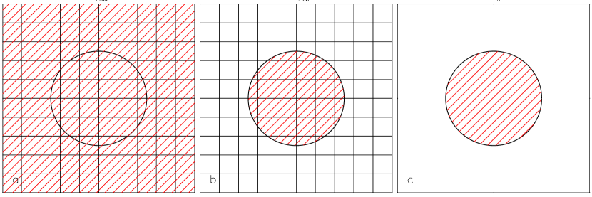
Figure 4: Sequence of the force calculations for the hybrid PM/high resolution (HR) code. The inner sphere corresponds to the HR region, the shaded area indicates those parts of the simulation box which are involved in the force calculation; a) The PM force with periodic boundary conditions ${\bf F}_{\rm PM,p}$ is computed for all particles, b) only for particles of the lower three mass hierarchies, the PM force with vacuum boundary conditions ${\bf F}_{\rm PM,v}$ is calculated and subtracted from ${\bf F}_{\rm PM,p}$, c) the HR code is used to calculate high resolution forces ${\bf F}_{\rm HR}$ again only for the particles of the lower mass hierarchies. The total force for these particles is given by ${\bf F}_{\rm PM,p}-{\bf F}_{\rm PM,v}+{\bf F}_{\rm HR}$.

The PM forces ${\bf F}_{\rm PM,p}$ and ${\bf F}_{\rm PM,v}$ are calculated on $32^{3}$ mesh via Fast Fourier transforms. Particles are assigned to the grid using TSC assignment (Efstathiou et al.  1985). Since for ${\bf F}_{\rm PM,v}$ less than 1/8th of the volume of the mesh is occupied, vacuum boundaries can be easily implemented in the PM calculation (Eastwood & Brownrigg 1979). Beside the periodic images, the mesh forces within the high resolution region is exactly zero and the short range forces obey a Newtonian force law. Therefore, our hybrid scheme is different from the classical P3M approach, where the short range force is a correction to the mesh force and, therefore, it does not follow a $1/r^{2}$ law. Furthermore, no matching error at the maximum radius of the PP correction is involved (Efstathiou et al.  1985).

Throughout a simulation, the way how forces are calculated are not changed for every individual particle: for the highest mass hierarchy, the force is always ${\bf F}_{\rm PM,p}$, for the lower three mass hierarchies always ${\bf F}_{\rm PM,p}-{\bf F}_{\rm PM,v}+{\bf F}_{\rm HR}$. No discontinuities matching two different numerical schemes together are involved. A potentially pathological case may occur, if particles of the lower mass hierarchies move outside the central box of side length $r_{\rm box}/2$. The vacuum PM force for those particles is then not properly represented. An additional tidal field arises since the periodic images of these particles are not properly compensated. The high resolution region, however, is situated around a galaxy cluster and it therefore covers an overdense region. Only rarely, if at all do particles of the lower three mass hierarchies leave the central sphere of radius $r_{\rm box}/4=62.5\,h^{-1}$Mpc, as also can be seen in figure 5. Particles of the highest mass hierarchy which move into the high resolution sphere are less problematic. Due to the low resolution of the PM force, their perturbing effect is rather limited. As can be seen in figure 5, the mixing between different mass hierarchies is rather limited and only neighbouring hierarchies interact. The largest mass difference between closely interacting particles is thus only factor of eight and relaxation effects are only weak. Furthermore it can be seen that the minimum radius which a particle of the second mass hierarchy achieves is still a factor of 3 larger than the virial radius of the galaxy cluster at $z=0$. Thus the galaxy cluster and its environment is consistently simulated with the highest resolution and perturbing relaxation effects due to accidently intruding more massive particles can be excluded.

Finally we note, that the level within the mass hierarchy at which the force calculation is switched from the PM to the high resolution force is to some extent arbitrary. For the combination of PM with a GRAPE-PP code (this code is used for the simulations presented in this paper) it is computationally advantageous to use PM only for the highest mass hierarchy. The PM part has thoroughly to be performed on the (relatively slow) front end, while the PP part benefits from the high performance of GRAPE. For a similar code on a conventional computer, which uses a tree code for the short range forces, the opposite is true: the calculation of the short range forces is more expensive than the PM part. It is likely to be more advantageous to use a finer grid and to calculated not only the highest mass hierarchy by PM but also some of the lower ones.

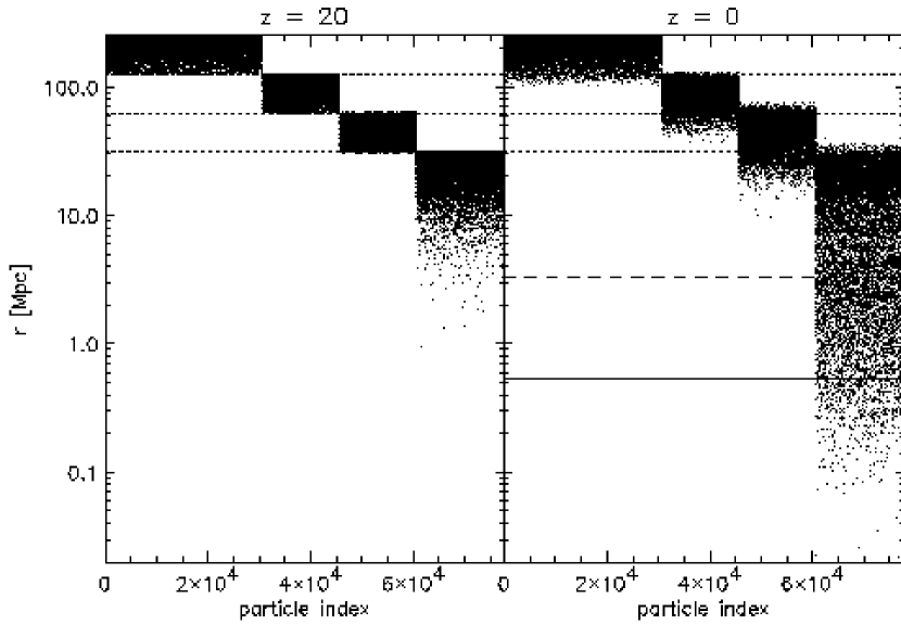
Figure 5: Radius $r$ of a particles at the begin (left) and the end of the simulation. The dashed line corresponds to the virial radius, the solid line to the scale radius of the cluster at $z=0$. The three dotted lines correspond to the outer radii of the lower three mass hierarchies at $z=z_{\rm init}$. As can bee seen, mixing of particles across the boundary of the highest mass hierarchy is only weak. No particle of the upper three mass hierarchies can be found within $3r_{\rm vir}$.

3.2.2 The influence of gravitational softening, time stepping and boundary conditions

The high resolution force is softened according to a Plummer law. The softening length is set to $\epsilon_{\rm ref}=12.5\;h^{-1}\,$kpc. The time evolution of the N-body system is integrated by a leap frog time integrator. The time step is set to

$$\Delta t_{\rm ref}=\frac{\epsilon_{\rm ref}}{\max_{i}(|{\bf v}_{i}|)}\,,$$ (6)

${\bf v}_{i}$ being the velocity vector of particle $i$. Because the PM calculation consumes a substantial part of the total CPU time per time step, we do not use an individual time step scheme.

In order to study the influence of numerical parameters, smoothing length and time step criteria are varied and their influence on the structure of a halo is investigated. For CPU economy reasons, these test simulations use only particles of the lowest mass hierarchy and vacuum boundary conditions. Initial displacements and velocities are identical to the CDM C realisation.

In figure 6a we demonstrate the effect of gravitational softening on the density stratification inside a halo plotting the profiles of $r^{2}\varrho$. The binning of the particles is described in detail in section 3.3.2. The softening length $\epsilon$ is varied between $0.2\epsilon_{\rm ref}$ and $8\epsilon_{\rm ref}$. To fix the number of time steps to nearly the same value (about 4000 time steps) the time step is set to $\Delta t=\beta\frac{\epsilon}{\max_{i}(|{\bf v}_{i}|)}$ with $\beta$ varying between 5 and 0.125 correspondingly. The reference softening $\epsilon_{\rm ref}$ corresponds to less than 1% of the virial radius of the test halo. As can be seen, the results are fairly converged for a softening between $0.4\epsilon_{\rm ref}$ and $\epsilon_{\rm ref}$. For the model with $\epsilon=2\epsilon_{\rm ref}$ slight while for the model with $\epsilon=8\epsilon_{\rm ref}$ a substantial depletion of the density near the center ($r<0.3\,h^{-1}$ Mpc) can be observed, though the density distribution at large scales is still fairly well represented. In the case of the smallest softening length $\epsilon=0.2\epsilon_{\rm ref}$ significant deviations can be observed. This demonstrates the importance of the number of time steps, the simulation has too small a number of time steps to handle the strong interparticle forces which can arise for such a small softening length. Close two body encounters result in high energy particles which escape the halo.

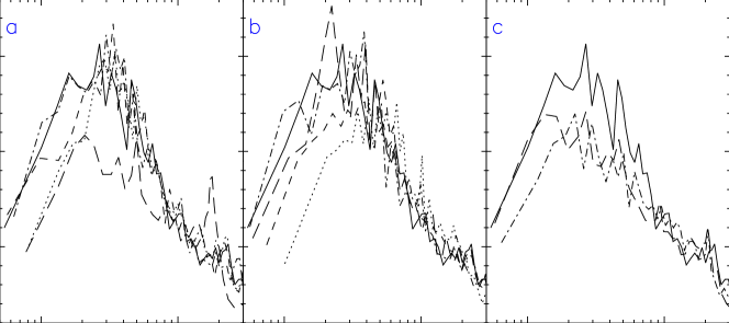
Figure 6: The influence of softening, time stepping and boundary conditions are tested on the density stratification inside a halo. The profiles of $\varrho\,r^{2}$ as function of $r$ are plotted for different test simulations. Plot a) shows the profiles for different plummer softening, $\epsilon=\epsilon_{\rm ref}$ (solid), $2\epsilon_{\rm ref}$ (dashed), $0.4\epsilon_{\rm ref}$ (dash dotted), $8\epsilon_{\rm ref}$ (dotted) and $0.2\epsilon_{\rm ref}$ (long-dashed dotted), plot b) for different time stepping: $\Delta t=\Delta t_{\rm ref}$ (solid), $0.25\Delta t_{\rm ref}$ (dash dotted), $4\Delta t_{\rm ref}$ (long dashed), $8\Delta t_{\rm ref}$ (dashed) and $10\Delta t_{\rm ref}$ (dotted), plot c) for different boundaries conditions: isolated boundaries at $r=r_{\rm box}/16$ (solid) and at $r=r_{\rm box}/4$ (dashed) and periodic boundaries (dash dotted).

In figure 6b the influence of the time stepping is investigated. Fixing the smoothing length to $\epsilon=\epsilon_{\rm ref}$ five simulation are done with $\Delta t=\Delta t_{\rm ref}$, $\Delta t=0.25\Delta t_{\rm ref}$ $\Delta t=4\Delta t_{\rm ref}$ $\Delta t=8\Delta t_{\rm ref}$ and $\Delta t=10\Delta t_{\rm ref}$. The profiles of $\varrho\,r^{2}$ for $\Delta t\leq 4\Delta t_{\rm ref}$ show no clear deviation from each other. But for $\Delta t>4\Delta t_{\rm ref}$ the central region is not as compact as for the smaller time step criteria. This indicates that the chosen time stepping is sufficiently finely grained.

The influence of the boundary conditions is investigated by comparing three simulation (initial conditions as in model CDM C) under differing boundary conditions. One simulation uses periodic boundary conditions (BC), one uses vacuum boundaries at the boundary of the highest resolution sphere (inner $31.25\,h^{-1}$Mpc sphere) (VC1) and one vacuum boundaries at the boundary of the third mass hierarchy (inner $125\,h^{-1}$Mpc sphere) (VC3). The simulation BC was performed with the hybrid PM/GRAPE scheme presented above, while for the runs VC1 and VC3 the PM part has been disabled. All other numerical parameters are kept identical for all runs, i.e. $\epsilon=\epsilon_{\rm ref}$ and $\Delta t=\Delta t_{\rm ref}$.

In figure 6c, $\varrho\,r^{2}$ is compared for all three models. They agree well above $r\approx 1\,h^{-1}$ Mpc but show clearly differences in the central region. The halo center becomes less dense with increasing surrounding matter and even a slight difference in the central density between model BC and VC3 can be observed. This demonstrates the importance of properly including large scale matter distribution in such simulations. As we will discuss in section 5.3, the gravitational field exerted by surrounding matter may play a critical role for the density distribution of dark matter haloes.

In summary these results show that the influence of different numerical parameters is fairly well understood. For parameters close to the reference values proposed above, the density profiles are consistent with each other. Within the numerical discretisation errors, the choice of a specific code and/or a specific type of softening does not affect the results of the simulations. Nevertheless, the total number of time steps of about $10^{4}$ is still moderate and allows us to investigate a fairly large sample of cosmological models, each of which represented by several sets of initial conditions.

3.3 Miscellaneous

3.3.1 Identification of haloes and substructure

Later in this paper, the formation history of haloes will be investigated. The mass of the most massive progenitor as well as the mass in collapsed structure will turn out to be a valuable tool to characterise the merging histories of individual haloes. In order to identify collapsed substructures and to label those particles which belong to such a structure, we use a group finding algorithm which is based on a binary tree structure similar to that of a N-body code. In a binary tree, pairs of mutually nearest neighbours are grouped to nodes, mutually neighbouring nodes to more massive nodes and so on. These procedure is iteratively repeated until only one node containing all particles remains (for details see Porter 1985; Jeringhan & Porter 1987; Steinmetz & Müller 1993). The nodes preferentially cover regions of high particle density. The estabilshed hierarchy of nodes is now scanned for nodes which can be identified as bound objects. Nodes which do not have at least virial density $\varrho_{\rm vir}(z)$ or which consist of less than $10$ particles are eliminated. The volume of a node is approximated by the volume of its ellipsoid of inertia. From the remaining list of nodes, all those are discarded which do not enclose a compact mass accumulation. The compactness of a node is inferred by measuring the mass within $r_{\rm core}=25\;h^{-1}\,$kpc near the center of mass of the considered node. The average density within $r_{\rm core}$ is then required to be larger than the average density of the considered node. Furthermore any subnode of these nodes must not be underdense. This procedure delivers a list of nodes (i) which are not a subset of a compact, more massive node and (ii) which are part of collapsed bound structures. The advantage of our new algorithm is that close halo pairs can be resolved.

3.3.2 Radial matter distribution of haloes

In section 5.1 we will discuss the matter distribution of haloes. The density profile is measured by binning the particle distribution in 200 spherical shells centered on the minimum of the cluster potential. Each shell contains $N$ particles, where $N$ is logarithmically increasing with radius starting with $N=120$ near the center. At $z=0$, the bin at $r_{\rm vir}$ contains about $140$ particles. For the mixed dark matter models twice as many particles per bin have been used. Each bin is assigned a radius corresponding to the average distance of all particles which belong to the bin. This radius is smaller than the half-volume radius of a shell, since the density decreases with distance from the cluster center. The use of spherical bins for triaxial structures like clusters has no affect on the shape of profiles (Lemson 1995).

The radial density distribution can sensitively depend on the definition of the halo center. We use the minimum of the gravitational potential to define the halo center. This halo center usually coincides with that defined by the maximum density or the center of mass, but for bimodal mass distributions (as typically occur during merging events) they can differ substantially. While for a bimodal mass distribution the minimum of the gravitational potential focuses on one of the two subclumps, the center of mass is located between the two contributing subclumps. Binning the mass distribution in radial shells centered on the center of mass thus results in an artificially shallow density distribution near the halo center. Compared to the maximum density, the minimum of the potential has the advantage to select the most massive progenitor as the center, while the maximum density can correspond to a small clump of high central density.

The potential minimum of cluster is defined in the following way: The gravitational potential of each contributing particle is assigned to a $32^{3}$ cube grid using NGP charge assignment (Eastwood et al.  1980) and the mesh cell with the lowest potential is identified. The center of a halo is then defined as the mean value of the potential weighted positions of all particles inside a sphere around the cell center with a radius equals to half the cell size.

The outer boundary of a cluster is defined by the virial radius $r_{\rm vir}$, the radius at which the mean overdensity within a sphere equals the virial density $\varrho_{\rm vir}$ of the spherical top-hat model (equation 5). All particles which lie inside $r_{\rm vir}$ are taken to belong to the cluster.

4 The process of structure formation

This section investigates merging history, shape and angular momentum of clusters. Variations between different clusters of a given scenario, as well as between clusters from different cosmogonies are discussed. We consider first the qualitative nature of cluster collapse as it arises in our simulations.

4.1 Mergers and mass accretion

The formation of a cluster can be followed by looking at the distribution of those particles which at the present epoch lie within a sphere of radius $r_{\rm vir}$. In figure 7, the particle positions projected in the x-y plane are shown for the realisation A of the CDM, LCDM, OCDM, CHDM III and HDM models. The particle distribution is shown at redhsifts $z=18.7,1.84,0.53,0.24,0$. The selected models represent typical evolution patterns for the various cosmological parameters. Some differences between the CDM, LCDM and OCDM can be seen, in particular the earlier collapse and greater compactness of the OCDM cluster at $z=1.84$ and $0.53$. The largest differences are between various cold dark matter clusters on the one hand, and the CHDM III and HDM clusters on the other. The latter models form distinct structures only at redshifts $z<1$.

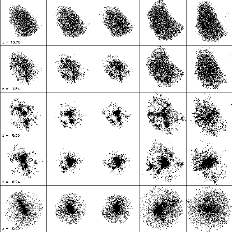
Figure 7: Distribution of particles of cluster A (at $z=0$ ) of the CDM, LCDM, OCDM, CHDM III and HDM cosmogony at $z=19$, $1.8$, $0.5$, $0.2$ and $0$ (from above). The physical size of the corresponding boxes is $1.7$, $9.1$, $11.4$, $9.5$ and $4.5\,h^{-1}{\mathrm{M}pc}$.

In the cold dark matter models the clusters of each realisation follow coarsely the same evolution pattern. Covering initially an ellipsoidal shaped region the particles in realisation A accumulate first along filamentary structures. Within the filaments several small spherical shaped objects of similar mass are formed. These structures preferably merge at the intersections of the filaments. A few clumps of successively larger mass are built up, and following a central impact they merge together. Smaller clumps are tidally disrupted during the infall on the central matter accumulation. The nonlinear evolution is fastest in the OCDM model, where distinct objects are visible in the filaments already at $z\approx 4$. Roughly the same degree of clustering is reached in all EdS-models at later times. This holds even for the mixed dark matter models, where the presence of a hot component delays the growth of structure. The similarity of the clustering pattern at late epochs is largely due to the normalisation of all models to $\sigma_{8}=0.63$, i.e. the linear overdensity is identical on a length scale only moderately larger than a typical cluster scale.

However, the formation history can be quite different for different realisations. This is shown in figure 8, where the formation history of the OCDM cluster is shown for all three realisations A, B and C. The initial particle distribution seem to be more spherical for realisation B and C, although this is partly a projection effect. Realisation B is elongated in the y-z plane by an amount similar to the x-y elongation of realisation A, while realisation C is less elongated in both projections. At lower redshifts, the particle distribution also appears less filamentary for realisations B and C, but for realisation B the orientation of the filament is along the line of sight. In realisation B and C, a massive clump has established relatively early near the center and the future evolution of the cluster can be well characterised by accretion of outer matter shells, similar to the spherical collapse model.

Figure 8: Distribution of particles of the most massive cluster (at $z=0$ ) of all three OCDM realisation A (upper row), B (middle row) and C (lower row) at $z=19$, $1.8$, $0.5$, and $0$ (from left). The physical size of the corresponding boxes is $1.4$, $6.4$, $7.7$ and $2.9\,h^{-1}{\mathrm{M}pc}$.

This visual impression can be quantified by looking at the mass ratios of the progenitors of the $z=0$ cluster. The progentiors of a halo are found using the halo identification techniques described in section 3.3.1 for every output. Each collapsed object for which more than half of its particles end up in the cluster at $z=0$, defines a progenitor. Figure 9a shows the mass ratio of the most massive progenitor $M_{pr,max}$, to the total cluster mass $M_{cl}$ at $z=0$ as a function of redshift. This ratio represents the nonlinear growth of the cluster. Consistent with the expectation of linear theory, the low $\Omega$ models exhibit a faster growth of structure at high redshifts as compared to the $\Omega=1$ CDM models. The growth rate of mixed dark matter models is somewhat suppressed at higher redshifts due to the influence of the hot component.

A good measure for the merging history of a cluster is the ratio of the mass of the most massive progenitor $M_{pr,max}$, to the mass of all (collapsed) progenitors $M_{pr,all}$. If a halo grows only by accumulating (not collapsed) infalling matter this ratio would be one at all times. Departures from one are a sign of mergers. The degree of departure is governed by the number and mass ratio of the progenitors and thus to the merger rate. Figure 9 b) shows the ratio $M_{pr,max}/M_{pr,all}$ for our clusters.

Figure 9: a) Mass fraction of the most massive progenitor to the total cluster mass and b) ratio of the mass of the most massive progenitor to the mass of all gravitational bound sub-clumps as function of redshift. As in figure 2 the solid line corresponds to CDM,the dash triple-dotted to LCDM, the long-dashed to OCDM, the thick dotted, dash dotted and dashed line to CHDM I, II and III, and the thin dotted line to the HDM model.

While the redshift dependence of the cluster mass is very similar for the different realisations, its merging history is very different (figure 9b). For realisation A, the ratio $M_{pr,max}/M_{pr,all}$ lies close to its minimum for a long time and the most massive progenitor comprises only about 50-60% of the mass in all collapsed objects. This reflects the visual impression from figure 7 that the cluster has several progenitors of similar mass which merge together at a redshift close to zero. Realisation B and especially C exhibit much less merging events and the total amount of mass in collapsed structures is largely dominated by the most massive progenitor, consistent with figure 7 which shows for these realisations a dominant mass concentration near the center. The differences in the merging histories between differing cosmological models are much less than those between different realisations and they are barely significant. Such a similarity in the evolution pattern is also predicted by the modified Press-Schechter model (Bond et al.  1991, Lacey & Cole 1993), which predict identical merging trees (number of mergers) for Gaussian fields with identical phases. Different cosmological models differ primarily in the different assignment of an individual merging event with a physical time coordinate, i.e. the differing redshift dependence of $M_{*}(z)$.

4.2 Shape and angular momentum of the haloes

Figure 10: Time evolution of the size $R$, the mass ratio $M_{vol}/M_{cl}$, the axes ratio $b/a$ and $c/a$ and the spin parameter $\lambda$ of the region occupied by the particles which end up in a halo at $z=0$. The CDM clusters correspond to the solid lines, LCDM clusters to the dash triple-dotted lines, OCDM clusters to long-dashed lines, the clusters of the three CHDM models to the thick dotted (I), dash dotted (II) and dashed (III) and the HDM clusters to the thin dotted lines. The straight dotted line indicates the growth of $\lambda$ proportional to $(1+z)^{-1}$.

Further aspects of cluster collapse can be studied by investigating the mass distribution within the volume ${\mathcal{V}}(z)$, defined as the volume covered by those particles which at $z=0$ lie within the virial radius $r_{\rm vir}$ of the cluster (hereafter the cluster particles). The shape of ${\mathcal{V}}(z)$ deviates from a sphere at higher redshifts. We define the boundaries of ${\mathcal{V}}(z)$ by those cluster particles which have the largest distance to the center of mass of all cluster particles. To identify the boundary particles the volume around this center of mass is devided in its eight octants. Inside each octant the absolute values of the three space coordinates of each cluster particle are compared to the absolute coordinates of all other cluster particles. A particle lies inside ${\mathcal{V}}(z)$, if one of the remaining particles has a larger absolute coordinate in one direction than the reference particle. With the same method one can also select all particles inside ${\mathcal{V}}(z)$ by comparing the coordinates of all particles with those of the boundary particles. We then approximate ${\mathcal{V}}(z)$ by its ellipsoid of inertia (principal axes $a$, $b$, $c$) and define the size $R$ of the volume ${\mathcal{V}}(z)$ as the radius of a sphere with the same volume as the ellipsoid of inertia of ${\mathcal{V}}(z)$. $M_{\rm vol}$ is the mass enclosed by ${\mathcal{V}}(z)$. The angular momentum $L_{\rm vol}$ of the cluster region can be parametrised using the spin parameter $\lambda$. It can be generally defined as

$$\lambda=\frac{L_{\rm vol}}{G^{\frac{1}{2}}M_{\rm vol}^{\frac{3}{2}}R^{\frac{1}{2}}}.$$ (7)

This definition of $\lambda$ also works if the cluster region as a whole is not gravitionally bound. For virialized objects $G\,M_{\rm vol}/R$ gives roughly the total energy $E$ of the object thus leading to the usual definition of the spin parameter, $\lambda=L_{\rm vol}\sqrt{|E|}/(G\,M^{2.5})$.

In figure 10 the time evolution of the size $R$, of the axis ratios $b/a$ and $c/a$, of $M_{\rm vol}/M_{\rm cl}$ and of $\lambda$ is shown. These figures demonstrate again, that for hierarchical models the general picture of collapse is very similar within the same realisation, nearly independent of the cosmogony. Only the HDM clusters show departures from this picture.

In figure 11 $R(z)$ scaled with the turnaround radius $R_{ta}$ is explicitly compared to the solution of the top-hat model for the clusters of realisation A. For each halo the Tolman-Bondi equation (3) is solved using the mass inside ${\mathcal{V}}(z)$ at $z=20$ as the collapsing mass $M$. The energy $E$ is derived at turnaround, $E=GMR_{ta}^{-1}+\Lambda/6R_{ta}^{2}$. Before turnaround all models show a very good agreement between the numerical simulation and the spherical top hat model . After turnaround the analytical solution gets singular whereas simulated clusters virialise. In all cases the virial radius is approximately 40 % of the turnaround radius. But due to the definition of $R$ as the effective radius of the ellipsoid of inertia it also reflects the mass distribution inside the halo region. The strongly clustered matter distribution of the haloes leads to a smaller size than a homogeneous one of the same mass as assumed in the top-hat model. It is remarkable that the deviations from the top-hat solutions is smallest for HDM model. As discussed later the evolution of the HDM clusters is less violent than for the other models enabling an almost undisturbed infall of matter.

The collapse is initially driven by a mass which is $20-50\%$ larger than the halo mass at $z=0$. The deviation is least pronounced for realisation C which was shown to have a merging history most similar to a spherical accretion model. The surplus of mass is reduced at low redshift (between $z\approx 0.4$ and 0.1) when the collapse along the smallest axis of the ellipsoid of inertia has been completed and the axis ratio $c/a$ reaches its minimum. The lost mass is partly linked with particles which gain enough energy in the violent phase after collapse of the smallest axis to leave the halo. The residual mass forms small clumps which lie initially within ${\cal V}(z)$ (preferably at the end of the major axis of the ellipsoid of inertia) but do not participate in the collapse. In the final state of the halo collapse they are not enclosed by ${\cal V}(z)$ anymore.

Figure 11: Time evolution of the size $R$ of all haloes of realisation A (apart from the CHDM II model) compared to the time evolution of the spherical top-hat model of a sphere with the same initial mass and turnaround radius.

The evolution of the axis ratio of the ellipsoid of inertia shows the anisotropy of the collapse. It depends strongly on the local realisation of the initial conditions. In realisations A and C the collapse is faster only along the smallest axis, while the two longer axes remain nearly equal. In realization B on the other hand both small axes collapse faster than the major axis. As discussed in section 4.1 the clusters of realisation A are formed out of a very filamentary structures where all filaments lie in one sheet. Here the collapse perpendicular to the sheet (corresponding to the axis c) is faster than the merging of the clumps forming in the filaments. The same happens for the clusters of realisation C. The initial structure is less filamentary but forms a sheet. A different behaviour is observed for the realisation B, since here the clusters evolve out of two major objects forming one filament. The attraction of these two components needs more time than the collapse of each component alone.

The evolution of the spin parameter $\lambda$ is almost unaffected by the mass loss and the anisotropy of the collapse. It grows approximately proportional to the expansion factor $a=(1+z)^{-1}$, the same rate expected in linear theory. According to linear theory, the total angular momentum should grow like $a^{2}\dot{D}$ (White 1984, Steinmetz & Bartelmann 1995). Before turn around, $R\propto 1+z$, and therefore from the definition of $\lambda$ in equation (7) it grows to first order as $\lambda\propto a^{3/2}\dot{D}$. At high redshifts the Einstein-de Sitter relations $D\propto a$ and $a\propto t^{2/3}$ are approximately valid in all cosmological models lead to the $\lambda\propto(1+z)^{-1}$ dependence. Interestingly, as shown in figure 10 nearly all clusters follow this growth even at low redshift. The final values of $\lambda$ lie in the range $0.06-0.1$ for realisations A and B, and $0.01-0.02$ for realisation C. Several massive clumps are located in the neighbourhood of the clusters which form in realisation A and B causing relatively strong tidal fields. The shape of ${\mathcal{V}}(z)$ is quite elongated and thus ${\mathcal{V}}(z)$ possesses a high quadrupole moment which can be efficiently spun up by the tidal field. Realisation C on the other hand has no nearby massive object and the shape of ${\mathcal{V}}(z)$ is nearly spherical. The weak tidal effects can work only inefficiently and the resulting spin up of the halo is therefore small (White 1984; Steinmetz and Bartelmann 1995). Thus we find that the amplitude of $\lambda$ can vary significantly between different clusters in a given cosmogony, while the difference between different cosmogonies are again small.

The formation of the two HDM clusters is qualitatively different from the hierarchically clustering models. No bound objects are formed until $z\approx 1$, but the matter accumulates in a sheet, which lies roughly perpendicular to the major axis of ${\mathcal{V}}(z_{\rm init})$. The different orientation of the sheet and of ${\mathcal{V}(z_{\rm init})}$ is compensated during the collapse. A more spherical ellipsoid of inertia develops before the collapse along the smallest axis has finished. Therefore, the axis ratio of the ellipsoid of inertia increase at high redshifts (figure 10). The evolution of the spin parameter is much slower for HDM C. Due to the absence of nearby overdensities and the related tidal fields, angular momentum does not grow at high redshifts.

5 The structure of clusters

5.1 Cluster profiles at $z=0$

As shown in figures  7 and 8, galaxy clusters build up quite irregularly. The formation can be characterized by mergers of large clumps as in the case of realization A or by infall of less massive objects as in realization C. A smooth spheroidal matter distribution can only be observed near the center of the cluster, where the particle distribution has virialised. But even at low redshift matter infall and tidal fields are still present, especially in the case of the high $\Omega$ models.

We fit an NFW profile to the binned radial matter distribution. Fit parameters are determined using the the circular velocity $v_{\rm cir}(r)$ since it is less noisy. The circular velocity $v_{\rm cir,n}(r)$ of an NFW profile is given by

$$v_{\rm cir,n}^{2}(x)=4\pi G\varrho_{b}\delta_{n}a_{n}^{2}x^{-1}\left[\ln(1+x)-\frac{x}{1+x}\right]$$ (8)

with $x=r/a_{n}$. The circular velocity at the virial radius is $v_{\rm vir}=v_{\rm cir,n}(c)=\sqrt{GM_{\rm vir}/r_{\rm vir}}$ with $c=r_{\rm vir}/a_{n}$. Therefore $\delta_{n}$ is also a function of $a_{n}$ and the density profile depends only on one free parameter (Navarro et al.  1996).

The scale length $a_{n}$ is determined by means of a nonlinear least square fit weighted by the errors in the circular velocity for each bin. Errors are determined by means of a bootstrap method (Efron 1979) using a resampling rate of $100$. Each sample is binned using the same bin boundaries as the original particle distribution. Therefore the particle number and the mass within one bin varies and allows one to estimate the standard deviation in $v_{\rm cir}$. Calculating the bin error using the bootstrap method takes into account not only the discretisation error ($\propto 1/\sqrt{N_{bin}}$) but also the deviation of the halo region from a sphere. In table 3 all profile parameters of a halo are listed. We also give an error estimate for the characteristic radius $a_{n}$ derived form the bootstrap analysis. This error typically is of the order of 10 per cent. For CHDM clusters it is little bit smaller since the bins contain more particles.

Table 3: Profile parameters for the 20 considered clusters. Listed are the viral mass $M_{\rm vir}$, the virial radius $r_{\rm vir}$, the scale length $a_{n}$ with its 3$\sigma$ bootstrap error, the characteristic overdensity $\delta_{n}/4$ and the concentration $c=r_{\rm vir}/a_{n}$. (The number in the brackets give the error in $a_{n}$ as a percentage of $a_{n}$.)

Model	$M_{\rm vir}\,[10^{15}\;h^{-1}\;\Omega_{0}\;M_{\odot}]$	$r_{\rm vir}\,[h^{-1}\;{\rm Mpc}]$	$a_{n}\,[h^{-1}\;{\rm Mpc}]$	$\delta_{n}$	$c$
OCDM A	1.01	1.30	$0.23\pm 0.03$ (12%)	5950	5.76
OCDM B	0.91	1.25	$0.18\pm 0.02$ (10%)	10150	7.28
OCDM C	1.12	1.34	$0.18\pm 0.01$ (7%)	11550	7.63
LCDM A	0.95	1.34	$0.21\pm 0.03$ (12%)	7010	6.65
LCDM B	0.69	1.21	$0.20\pm 0.03$ (14%)	5820	6.12
LCDM C	1.11	1.42	$0.25\pm 0.03$ (14%)	4840	5.71
SCDM A	1.01	1.69	$0.42\pm 0.12$ (29%)	1260	4.11
SCDM B	0.71	1.50	$0.29\pm 0.05$ (16%)	2250	5.33
SCDM C	0.96	1.66	$0.28\pm 0.07$ (26%)	3180	6.19
CHDM I A	1.31	1.84	$0.41\pm 0.05$ (12%)	1530	4.52
CHDM I B	0.76	1.54	$0.30\pm 0.04$ (15%)	2150	5.20
CHDM I C	1.32	1.85	$0.35\pm 0.03$ (5%)	2360	5.48
CHDM II A	1.24	1.81	$0.49\pm 0.04$ (8%)	1030	3.76
CHDM II B	0.79	1.55	$0.30\pm 0.03$ (11%)	2250	5.31
CHDM II C	1.27	1.82	$0.30\pm 0.02$ (8%)	3280	6.32
CHDM III A	1.70	2.01	$0.63\pm 0.10$ (15%)	750	3.23
CHDM III B	0.99	1.66	$0.46\pm 0.05$ (10%)	1010	3.73
CHDM III C	1.26	1.82	$0.40\pm 0.02$ (6%)	1650	4.66
HDM A	1.78	2.04	$0.85\pm 0.12$ (14%)	420	2.46
HDM C	0.96	1.66	$0.45\pm 0.19$ (43%)	1070	3.83

In figure 12, $r^{2}\varrho(r)$ and the circular velocity $v_{\rm cir}(r)$ are shown as function of $x=r/a_{n}$ for all clusters at $z=0$. $r^{2}\varrho$ and $v_{\rm cir}$ are scaled to the value of the analytical fit at the scale radius. This enables a fair comparison of the haloes since under such a scaling all profiles which are fitted well by equation 1 should have identical shapes. The solid lines in figure 12 represent these reference profiles based on the NFW profile. All profiles are very well fitted by the NFW profile up to the virial radius. Larger deviations especially in form of spikes are produced by infalling subclumps (Tormen 1996), or due to incomplete relaxation as in the case of the HDM A. Both effects lead also to a larger error in $a_{n}$.

The general shape of the haloes follows the NFW profile is independent of the cosmogony. The only difference between the models is the concentration $c=r_{\rm vir}/a_{n}$ of haloes, characterized by the ratio of the viral radius to the scale length. $c$ is given in table 3 for all haloes. It can also be directly read off figure 12 looking at the x-values of the virial radii. A small value of $c$ means that the density in the center is lower compared to haloes with a high $c$. This is shown in figure 13, where the profiles of the circular velocity of the clusters of one realization are compared. For pure cold dark matter, there is a trend towards higher concentration from the CDM model to the LCDM and OCDM model. This trend can be well understood since the characteristic overdensity $\delta_{n}\propto(1+z_{f})^{3}$ (Navarro et al.  1996b) where $z_{f}$ is the formation time of the halo. In $\Omega<1$ universes structures form at an earlier epoch where the density of the universe is higher. The trend is most pronounced for the OCDM model, since in this scenario, structures form at the highest redshifts. There is also a strong correlation of $c$ with increasing influence of the hot component. The concentration becomes smaller as the hot dark matter becomes more dominant. Structure formation is retarded to very low redshifts.

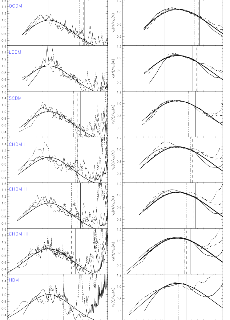
Figure 12: $\varrho(r)\,r^{2}$ and $v_{\rm cir}(r)$ of all clusters at $z=0$. All quantities are scaled to the values of the corresponding analytic expression at the scale radius $a_{n}$. The dash dotted, dashed and the long-dashed lines represent realizations A, B and C, respectively. The solid line gives the analytic expression using the parameters of the best fit to the NFW profile.

Figure 13: The profile of $v_{\rm cir}(r)$ is compared for all clusters of one realization at $z=0$. Now the distance is scaled with the virial radius $r_{\rm vir}$ and $v_{\rm cir}(r)$ with $v_{\rm vir}$. The lines are the same as in figure 2.

5.2 The asymptotic behaviour of the density profiles at large radii

Both the NFW and the Hernquist profile have been shown to provide a fairly accurate fit to the radial matter distribution of haloes formed in hierarchically clustering scenarios, though the NFW profile seem to provide a slightly better fit, especially at large radii. We investigate more quantitatively the asymptotic behavior at large radii using a generalized form of the NFW profile:

$$\frac{\varrho(r)}{\varrho_{b}} = \delta_{g}\frac{a_{g}}{r(1+\frac{r}{a_{g}})^{m}}\,,$$ (9)

$$v_{\rm cir,g}^{2}(x) = 4\pi G\varrho_{b}\delta_{g}a_{g}^{2}x^{-1}\times$$ (10)

$$\left[\frac{1+mx-x^{2}+mx^{2}-(1+x)^{m}}{(2-3m+m^{2})(1+x)^{m}}\right].$$

For $m=2$ the expression (8) has to be used for $v_{\rm cir,g}^{2}(x)$. We have thus introduced an additional free parameter $m$ which sets the asymptotic logarithmic slope $\alpha=m+1$ of the profile at large radii. $m=2$ and $m=3$ correspond to the NFW and the Hernquist profile, respectively. The physical meaning of the other two parameters, $a_{g}$ and $\delta_{g}$ is the same as that of $a_{n}$ and $\delta_{n}$ in the NFW profile, namely characteristic scale radius and central density.

By fitting equation (9) insidue $r_{vir}$ to the measured profiles for all available haloes we get the distribution of $m$. To enlarge the halo sample we include the most massive progenitor of each cluster identified in the outputs after $z=0.5$. With our sampling rate of one output per $\Delta a=0.05$ we get a total of $193$ haloes covering a mass range of $1.2\times 10^{14}h^{-1}\Omega M_{\odot}$ to $1.9\times 10^{15}h^{-1}\Omega M_{\odot}$. The halo sample of each cluster realization is not strictly independent as these haloes belong to the same evolution path. Due to the chosen sampling rate, however, the haloes are identified at different states of the evolution of a cluster. Each halo has included different amount of nonlinearities and represents a different state of relaxation. Furthermore, the asymptotic slope probes the outer part of a halo, which is mainly built up from the newly infalling matter. Though not strictly independent, our enlarged sample can be considered to represent the typical amount of scatter in the asymptotic behaviour at large radii.

The radial density distribution is similar in all of these objects as can be seen in figure 14. Here we plot the profiles of $v_{\rm cir}$ of the CDM A cluster at $z=0$ and of its most massive progenitors at seven earlier redshifts. The general shape of the profiles is comparable to the NFW profile, independent of redshift.

In figure 15 the number distribution $N(m)$ of the asymptotic slope of the profiles is plotted. The distribution is strongly peaked at $m=2$, the value of the NFW profile. This peak is a common feature for all cosmologies. There is no relation between $N(m)$ and redshift. We are thus led to conclude that the NFW profile has the best fit asymptotic slope at large $r$, for a generalized profile of the form of equation (9).

A different asymptotic behavior ($m\neq 2$) can be observed for haloes which participate in a merging event. Merging subclumps change the matter distribution along the infall direction, which is visible as spikes in the radial profile as mention earlier. Depending on the distance of the subclump relative to the halo center these spikes affect the asymptotic slope at large radii. A flattening of the profile results if a subclump is at radii slightly larger than $r_{\rm vir}$; on the other hand shortly after a subclump crosses $r_{\rm vir}$, the resultant spike leads to a steeper outer profile.

Figure 14: $v_{\rm cir}$ of the CDM A cluster at $z=0$ (solid line) and of its most massive progenitors at $z=0.05$ (dotted line), $0.10$ (dashed line), $0.17$ (dash-dotted line), $0.24$ (dash triple-dotted line) and $0.33$ long-dashed line). The smooth thick solid line correspond to the NFW profile.

Figure 15: Number distribution $N(m)$ for the asymptotic slope $m$ of the density profiles of all clusters and their most massive progenitors.

5.3 Non-radial motions and the evolution of the density profile

In the previous subsections we have demonstrated the universality of the measured density profiles of clusters. For $r<r_{\rm vir}$, the flattening below a certain scale length and the asymptotic decay of the profiles are well described for more or less relaxed haloes by the NFW profile. This general form of the radial density distribution in a halo is independent of redshift and the cosmological model. The evolution path of a single halo also does not appear to affect the profile. Recently Syer & White (1996) have argued that the inner slope of the universal density profile arises from repeated mergers. The clusters we have simulated however have very different merging histories; indeed the first collapsed objects and the entire haloes of our HDM simulations are formed without any significant mergers events. In this section we consider the role of non-radial motions in producing an NFW-like profile.

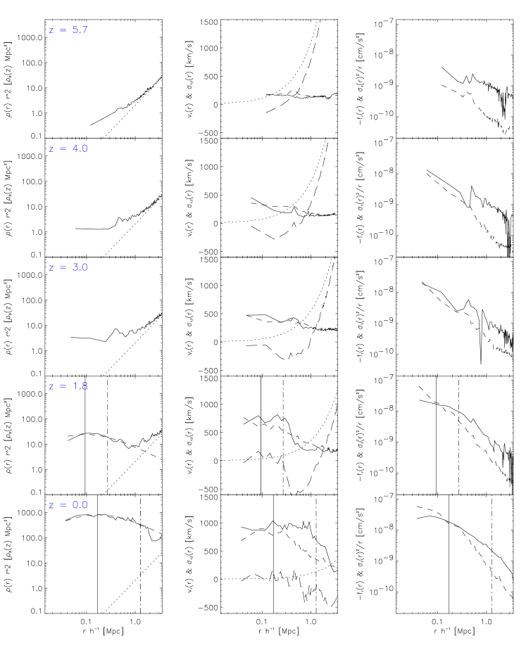
Figure 16: The formation of an NFW-like density profile is demonstrated with the OCDM C cluster. In the left panel the profile of $\varrho(r,z)r^{2}$ is plotted for the most massive progenitor. The NFW fit is the dashed curve, while the dotted line is for $\varrho(r)={\rm constant}$. The middle panel shows the profiles for the mean radial velocity $v_{\rm r}(r,z)$ (long dashed) and the radial $\sigma_{r}(r,z)$ (solid) as well as the transverse $\sigma_{t}(r,z)$ (dashed) velocity dispersion. The Hubble flow is indicated by the dotted line. In the right panel the negative radial gravitational force $f_{r}(r,a)$ (solid curve) is plotted together with the “centrifugal” force $\sigma_{t}(r,z)^{2}/r$ (long dashed curve). In the lower two rows the upright solid line shows $a_{n}$ and the dash dotted line $r_{\rm vir}$ at the given redshift.

It is illustrative to examine the time evolution of the density profile in parallel with the velocity structure of the halo as measured from the mean radial velocity $v_{r}(r)$, and the radial [$\sigma_{r}(r)$] and the transverse [$\sigma_{t}(r)$] velocity dispersion of particles. In figure 16 this evolution is shown for the OCDM C cluster. For the region where the most massive progenitor is formed, the profile of the density $\varrho(r)r^{2}$ is plotted as a function of distance $r$ at different redshifts (left panels). The middle panels shows the profiles of $v_{r}(r),\sigma_{r}(r)$ and $\sigma_{t}(r,z)$. The right panel shows the profile of $\sigma_{t}(r,z)^{2}/r$ in comparison with the radial component of the gravitational force.

Figure 16 shows how the development of a density profile like the NFW profile of equation 1 is accompanied by a transition from mainly radial infall of the halo particles to virialised motions with vanishing mean radial velocity. At $z=5.7$ all particles at radii below $0.3h^{-1}\,$Mpc have turned around and are falling towards the density maximum. The density profile is not much steeper than a constant density profile (the logarithmic slope $\alpha\simeq-0.8$). The first particles cross the central region before $z=4$ and move outwards again. Due to the overlap of the particles crossing the center for the first time and those which have fallen in and out several times, the density increases in the center as described by the secondary infall model (e.g. Bertschinger 1985). This results in the slope $\alpha$ becoming lower than $-2$ at radii below $0.2h^{-1}{\mathrm{M}pc}$. At $z\approx 3$ a large clump starts to merge with the progenitor, as evident by the spike in the density profile at $0.4h^{-1}$Mpc. By $z\simeq 2$ the slope has again become shallower than $-2$ in the center while it remains steeper than $-2$ for $a_{n}<r<r_{\rm vir}$. The shape of the density profile below $r_{\rm vir}$ remains almost stable up to $z=0$. Merging events temporarily disturb this matter arrangement, but the density distribution inside always returns to the NFW form.

The velocity structure near the center changes during collapse as shown in the middle panels of figure 16. Due to the mixing of inward and outward moving particles the mean radial velocity $v_{r}(r)$ in the central region approaches zero at $z=4$. After the first relaxed object has been formed (at $z\simeq 3$), $v_{r}(r)$ fluctuates around zero for $r<r_{\rm vir}$. The radial velocity dispersion $\sigma_{r}(r)$ increases with time at early times, but at late times ($z<1$) remains constant at nearly $1000$ km/s for all $r<r_{\rm vir}$. The transverse velocity dispersion $\sigma_{t}(r)$ remains approximately equal to $\sigma_{r}(r)$, though at late times it remains below $\sigma_{r}(r)$ in the outer parts of the halo. A “centrifugal” force, $f_{c}(r)=\sigma_{t}^{2}(r)/r$ can be associated with the transverse velocities. At $z=5.7$, the radial component of the gravitational force, $f_{r}(r)$ is approximately ten times larger in the center than $f_{c}(r)$, but it does not grow significantly (see the right panels of figure 16). It can be approximated by $-G\bar{\varrho}(r,z)\,r$, with the central mean density $\bar{\varrho}(r,z)$ remaining almost constant. By $z\simeq 2$, $f_{c}(r)$ becomes of the same order as $-f_{r}(r)$ for $r<a_{n}$, and it becomes larger at later times. A close examination of the redshift interval between $z=2$ and $z=0$ (not shown in the figure) reveals that there is very little variation in time in the profiles of $\sigma_{t}^{2}/r$ and $f_{r}(r)$: once the smooth profiles with a turnover at $r\simeq a_{n}$ are established they remain the same up to $z=0$.

The tangential velocities cause particles to move on orbits which can be locally described as Keplerian ellipses or hyperbolas. Typical particle trajectories do not pass close to the center if $f_{c}(r)$ is of the same order as $f_{r}(r)$ or larger, and if the transverse velocity of the particles is of order the radial velocity. Since particles at a given radius do not subsequently penetrate into the inner region of the halo they do not cause the density profile to steepen as much as it would if they were on radial orbits.

One can relate the orbit structure of halo particles to the density profile that arises in idealised models of secondary infall. The profile predicted by the purely radial infall model (Fillmore & Goldreich 1984; Bertschinger 1985) is close to what is observed in the outer parts of our haloes. In the inner parts however the profile is flattened owing to the significant tangential velocities, as described above. This flattening is consistent with the results of White & Zaritsky (1992) who included angular momentum into an infall model. They showed that whereas for purely radial infall, the profile does not become shallower than $\alpha=-2$, the inclusion of sufficient angular momentum can allow the profile to be arbitrarily shallow (depending on the initial profile). Their analytical model was restricted to scale-free conditions and had an artificial prescription for adding angular momentum. By construction their model led to power law final profiles. In contrast the initial power spectrum we use is not scale-free; there is no imposed spherical symmetry; and the angular momentum is acquired dynamically. Therefore we can only compare our profile to the predictions of infall models in a local, approximate sense.

The comparison is nevertheless interesting because the slope of the NFW density profile at $r=a_{n}$ is $\alpha=-2$, precisely the value at which the secondary infall model shows a transition from an infall profile dominated by radial motions, to one with significant tangential motions. We have shown in figure 16 that $r=a_{n}$ does mark a transition in the relative importance of the “centrifugal” force due to the tangential velocity dispersion and the radial component of the graviational force. The emergence of this transition coincides with that of an NFW-like profile with a slope that is shallower than $-2$ in the inner regions, and both features are stable over time once they appear at $z\sim 2-3$. Thus there are two qualitative changes in the density profile as haloes evolve from $z\sim 6$ to the present: the initial steepening as mainly radial infall sets in, and the subsequent flattening of the inner profile as tangential motions become significant. Both features are in accord with infall models, and do not appear to be disturbed by ongoing mergers. The same features are present in all the cluster haloes, and most significantly in the HDM haloes which have much less merging but produce very similar profiles. These qualitative features argue against the merger mechanism proposed by Syer & White (1996) to explain the formation of NFW-like profiles.

In the context of a violent relaxation scenario of halo formation, the non-radial motions of halo particles would be induced by mostly stochastic torques due to matter anisotropies. An alternative possibility is the radial orbit instability (e.g. Carpintero & Muzzio 1995) which exists even in the absence of large scale fluctuations in the potential. It is important to understand the origin of the torques that produce these tangential motions before they can be regarded as the dynamical agent in forming the density profile. We plan to experiment with halo collapse simulations from varying initial conditions to establish if the mechanism that produces an NFW-like profile is distinct from one in which mergers play the dominant role, though clearly both processes operate in the evolution of dark matter haloes.

6 Conclusions

We have investigated the formation and evolution of galaxy clusters in different cosmogonies by means of numerical simulations. The investigated cosmogonies include standard cold dark matter models ($\Omega=1$), open models ($\Omega=0.3$), models with a cosmological constant ($\Omega=0.3$, $\Lambda=0.7$), 3 mixed dark matter models with differing $\Omega_{\nu}$ and differing number of massive neutrino species as well as a pure hot dark matter model ($\Omega=1$). 3 different realisations of each model have been investigated. The simulation have been performed using newly developed high resolution N-body code which combines a PM code with a high resolution tree code or a direct summation N-body code based on the special purpose hardware GRAPE. High spatial and mass resolution is achieved by using an enhanced multi-mass technique and a hierarchically nested particle arrangement. Test simulations demonstrate that our chosen softening and time stepping are consistent and that results have numerically converged.

In all considered cosmogonies, except the hot dark matter model, structure forms due to hierarchical clustering. For identical phases of the Gaussian random field the evolution pattern of the halo formation is similar. Differences in the cosmological parameters and the power spectra mainly manifest in a different time evolution, but the merging pattern, like e.g. number of mergers and mass ratio of mergers is fairly similar. Consistent with the predictions of linear theory, the evolution proceeds earlier in models with $\Omega<1$, while in mixed dark matter models the evolution is retarded to low redshifts. As expected the evolution pattern of the HDM clusters is different as it is dominated by the initially smooth distribution of particles. The differences between individual realisations of a given cosmological model are large and much stronger than differences within differing cosmogonies for a given realisation. Gross properties of clusters like size or angular momentum can be well described by analytic models like, e.g. , the spherical top hat model.

At all considered redshifts, the density profile of the virialised portion of a galaxy clusters can be well described by the NFW profile (Navarro et al. 1996a), which has a slope of $\alpha=-1$ near the center and of $\alpha=-3$ at large radii. The NFW profile provides a very good description for all considered cosmogonies and the influence of the background cosmological model only influences the central matter concentration and the characteristic radius. Due to their earlier formation epoch, low $\Omega$ models are typically more concentrated than high $\Omega$ CDM modes. Analogously, mixed dark matter models are slightly less concentrated due to their retarded formation epoch. Our results extend earlier findings to other cosmological models and supports the interpretation that the NFW profile is generic for all hierarchically clustering scenarios. It is suggested that the characteristic radius $a_{n}$ and the shallow density profile ($\alpha>-2$) for $r<a_{n}$ are linked to the non-radial motions of particles. The mechanism that produces the tangential velocity dispersion of infalling particles and its possible dynamical role in the evolution of the density profile merits further investigation.

References

- [] Bardeen J.M., Bond J.R., Kaiser N., Szalay A.S., 1986, ApJ, 304, 15
- [] Bartelmann M., Steinmetz M., Weiss A., 1995, A&A, 297, 1
- [] Baugh C.M., Gaztanaga E., Efstathiou G., 1995, MNRAS, 274, 1049
- [] Bertschinger E., 1985, ApJS, 58, 39
- [] Bertschinger E., 1995, astro-ph/9506070
- [] Bond J.R., Kaiser, N., Cole, S., Efstathiou, G., 1991, ApJ, 379, 440
- [] Carpintero D.C., Muzzio J.C., 1995, ApJ, 440, 5
- [] Couchman H.M.P., 1991, ApJ, 368, 23
- [] Cole S., Lacey C., 1996, MNRAS, in press (astro-ph 9510147)
- [] Dubinski J., Carlberg R. G., 1991, ApJ, 378, 496
- [] Eastwood J.W., Brownrigg D.R.K., 1979, J. Comp. Phys., 32, 24
- [] Eastwood J.W., Hockney R.W., Lawrence D.N., 1980, Comp. Phys. Commun., 19, 215
- [] Efron B., 1979, A. Stat., 7., 1
- [] Efstathiou G., Davis, M., White, S. D. M., Frenk, C. S., 1985, ApJS, 57, 241
- [] Efstathiou G., Bond J.R., White S.D.M., 1992, MNRAS, 258, 1P
- [] Eke V.R., Cole S., Frenk C.S., 1996, MNRAS, 282, 263
- [] Ewald, P.P., 1921, Ann. Physik, 64, 253
- [] Filmore J.A., Goldreich P., 1984, ApJ, 281, 1
- [] Gunn J.E., Gott, J.R., 1972, ApJ, 176, 1
- [] Hernquist L., 1990, ApJ, 356, 359
- [] Hernquist L., Bouchet F.R., Suto Y., 1991, ApJS, 75, 231
- [] Hoffman Y., Shaham J., 1985, ApJ, 297, 16
- [] Hoffman Y., 1988, ApJ, 328, 489
- [] Jernigan J.G., Porter D.H., 1989, ApJS, 71, 871
- [] Katz N., White S.D.M., 1993, ApJ, 412, 455
- [] Klypin A., Holtzman J., Primack J.R., Regos E., 1993, ApJ, 416, 1
- [] Lacey C., Cole S., 199, MNRAS, 262, 627
- [] Lemson G., 1995, Ph.D. thesis, Univ. of Groningen
- [] Navarro J.F., Frenk C.S., White S.D.M., 1995, MNRAS, 275, 720
- [] Navarro J.F., Frenk C.S., White S.D.M., 1996a, ApJ, 462, 563
- [] Navarro J.F., Frenk C.S., White S.D.M., 1996b, submitted to ApJ (astro-ph/9611107)
- [] Peebles, P.J.E., 1980, The Large Scale Structure of the Universe, Princton
- [] Peebles, P.J.E., 1993, Principles of Physical Cosmology, Princton
- [] Porter, D.H., 1985, PhD Thesis, University of California, Berkeley
- [] Steinmetz M., Bartelmann, M., 1995, MNRAS, 272, 570
- [] Steinmetz M., Müller E., 1993, A&A, 268, 391
- [] Steinmetz M., White, S.D.M., 1996, MNRAS, in press (astro-ph/9609021)
- [] Syer D., White S.D.M., 1996, submitted to MNRAS (astro-ph/9611065)
- [] Sugimoto D., Chikada Y., Makino J., Ito T., Ebisuzaki T., Umemura M., 1990, Nature, 345, 33
- [] Tormen G., Bouchet F.R., White, S.D.M., 1996, MNRAS, in press (astro-ph 9603132)
- [] White S.D.M., 1984, ApJ, 286, 38
- [] White S.D.M., Zaritsky D., 1992, ApJ, 394, 1
- [] White S.D.M., Efstathiou G., Frenk C.S., 1993, MNRAS, 262, 1023
- [] White S.D.M., 1996, in Schaeffer R., Silk J., Spiro M., Zinn-Justin J., ed., Les Houches Session LX: Cosmology and Large-scale Structure, North-Holland, p. 349
- [] Zel’dvich Y.B., 1970, A&A, 5, 84