Signatures of Topological Defects in the Microwave Sky: An Introduction

An introduction to topological defects in cosmology is given. We discuss their possible relevance for structure formation. Especial emphasis is given on the signature of topological defects in the spectrum of anisotropies in the cosmic microwave background. We present simple analytic estimates for the CMB spectrum on large and intermediate scales and compare them with the corresponding approximations for models where initial perturbations are generated during an inflationary epoch.

1 Introduction

The formation of structure in the universe is one of the mayor open problems in cosmology. Already in 1946 Lifshitz has noted $\!{}^{{\bf?}}$ that expansion counteracts gravitational attraction in such a way, that in an expanding universe the gravitational potential cannot grow by linear gravitational instability. Also the growth of density perturbations is reduced to a power law due to expansion. In a radiation dominated universe, radiation pressure inhibits any significant growth of density fluctuations. In all, density fluctuations can have grown at most by a factor $\sim a_{0}/a_{\rm eq}=z_{\rm eq}\sim 10^{4}$ due to linear gravitational instability, where $a_{0}$ denotes the value of the cosmological scale factor today and $a_{\rm eq}$ denotes its value at the time of equal matter and radiation.

Therefore, initial fluctuations on the order of $10^{-4}$ caused by some other mechanism than gravitational instability are needed. Such initial fluctuations can then be enhanced by gravity and lead to density fluctuations of order unity and finally to the observed structures in the universe. Currently two classes of models which can generate initial perturbations are under investigation.

In the first class, initial perturbations emerge from quantum fluctuations of a scalar field, which expand during a period of inflation to scales larger than the Hubble scale and then “freeze in” as classical fluctuations in the energy density. Generically, inflationary models lead to a so called Harrison-Zel’dovich spectrum of fluctuations$\!{}^{{\bf?}}$. This spectrum is defined by the requirement of having constant mass fluctuations at horizon crossing:

$$\left\langle\left({\delta M\over M}\right)^{2}_{k_{H}(t),t}\right\rangle=\mbox{ constant,}$$ (1)

where $k_{H}(t)=2\pi/t$ denotes the wave number corresponding to the horizon scale at time $t$.

In inflationary models, initial fluctuations typically are Gaussian, i.e., with random initial phases. After inflation they evolve deterministically according to homogeneous linear cosmological perturbation equations. The evolution of an arbitrary mode $k$ of a perturbations variable $\delta$ can thus be described by means of a deterministic transfer function $T$ and the initial value $\delta(t_{i})$ is perfectly coherent with $\delta(t)=T(t,t_{i})\delta(t_{i})$. In other words

$${\langle|\delta(t_{i})\delta(t)|\rangle\over\sqrt{\langle|\delta(t_{i})|^{2}\rangle\langle|\delta(t)|^{2}\rangle}}={\langle|\delta(t_{i})T(t,t_{i})\delta(t_{i})|\rangle\over\sqrt{\langle|\delta(t_{i})|^{2}\rangle\langle|T(t,t_{i})\delta(t_{i})|^{2}\rangle}}=1~{}.$$ (2)

In the second class of models, perturbations are induced by topological defects which may form during a symmetry breaking phase transition. This mechanism is explained in the next section. The amplitude of initial fluctuations due to topological defects which form at a symmetry breaking energy scale $\eta$ is on the order of $\epsilon=4\pi G\eta^{2}$. To obtain the correct amplitude thus requires defects which form during a phase transition at GUT scale $\eta\sim 10^{16}$GeV.

In this situation, perturbations in the cosmic fluid are constantly sourced by topological defects and evolve according to inhomogeneous linear perturbation equations. Since the defects make up only a small perturbation of the cosmic energy density and since (soon after the phase transition) they do not interact with the cosmic fluid other than gravitationally, they evolve according to the unperturbed geometry (in linear perturbation approximation). However, defect evolution is in general non-linear and the random initial conditions of the source term in the linear cosmological perturbation equations of given scale $k$ ’sweep’ into other scales. Therefore, the perfect coherence of inflationary perturbations is no longer maintained and Eq. (2) is violated. How strong and how significant this decoherence is, depends on the details of the model considered.

Due to this general behavior inflationary models are sometimes called ’coherent’ and ’passive’ (no source terms in the linear perturbation equation) while defect models are called ’decoherent’ and ’active’ (fluid perturbations are constantly sourced by the defect energy momentum tensor) $\!{}^{{\bf?}}$. In this talk, we concentrate on the second class of models. The main similarities and differences of the two classes are summed up in table 1.

Inflationary models	Topological defects
Similarities
$\bullet$ Cosmic structure formation is due to gravitational instability of small
’initial’ fluctuations. $\rightarrow$ Gravitational perturbation theory
can be applied.
$\bullet$ GUT scale physics is involved in generating initial fluctuations.
$\bullet$ The only relevant ’large scale’ is the horizon scale. $\rightarrow$ Harrison-
Zel’dovich spectrum.
Differences
$\bullet$The amplitude of fluctuations	$\bullet$The amplitude of fluctuations
depends on details of the inflatio-	is fixed by the symmetry breaking
nary potential $\rightarrow$ fine tuning.	scale $\eta$, $\epsilon=4\pi G\eta^{2}$.
$\bullet$The linear perturbation eqs. are	$\bullet$The linear perturbation eqs. are in-
homogeneous (passive).	homogeneous, have sources (active).
$\bullet$For given initial perturbations,	$\bullet$The source evolution is non-linear
the entire problem is linear.	at all times.
$\bullet$Randomness enters only in the	$\bullet$Randomness enters at all times due
initial conditions.	to the mixing of scales in the non-
	linear source evolution (sweeping).
$\bullet$The phases of perturbations at	$\bullet$Phases may become incoherent.
a given scale $\lambda$ are coherent.
$\bullet$There exist correlations on super	$\bullet$No correlations on super Hubble
Hubble scales.	scales.
Perturbations are ’acausal’.	Perturbations are ’causal’.

Table 1: Similarities and and differences of inflationary perturbations versus perturbations induced by seeds.

2 Topological Defects

Topological defects are as ubiquitous in physics as are symmetry breaking phase transitions. Usually they are described by means of a scalar field (order parameter, Higgs field) evolving in a temperature dependent potential. In the Landau Ginzburg theory of super-conductivity, e.g., the order parameter represents the “Cooper pairs” which are described by means of a complex scalar field. In this example, the scalar field is electrically charged and interacts with the electromagnetic gauge field. For sake of simplicity, we consider here a pure scalar field $\phi$, with $\phi^{4}$ interaction term but without gauge field. If $\phi$ is in a thermal bath at temperature $T$ and we have ’integrated out’ the excitations of energies $E\ll T$, we obtain an effective Lagrangian density with temperature dependent potential $\!{}^{{\bf?},{\bf?}}$

$${\cal L}(\phi)={1\over 2}(\partial_{\mu}\phi)^{2}-V_{T}(\phi)~{}.$$ (3)

At very low temperature $V$ approaches the zero temperature potential, $V_{0}={1\over 4}\lambda(|\phi|^{2}-\eta^{2})^{2}$ with vacuum manifold

$${\cal M}_{0}=\{\phi\left||\phi|^{2}=\eta^{2}\}\right.~{}.$$ (4)

(The vacuum manifold denotes the space of minima of the potential $V$.) At higher temperatures, there are corrections to $V$ which in general depend on the interactions of the scalar field with other (fermionic and bosonic) fields. In our simple case, the main correction is of the form $T^{2}\phi^{2}$ which, at high enough temperature, namely for $T>T_{c}=2\eta$, changes the ’Mexican hat’ into a parabolic shape with ${\cal M}_{0}=\{0\}$.

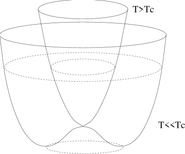
Figure 1: The temperature dependence of potential of a complex scalar field. The vacuum manifold is a circle for $T<T_{c}$ and a point for $T>T_{c}$.

At $T>T_{c}$ therefore, not only the Lagrangian density but also the only possible vacuum state $<\phi>=0$ is symmetric under phase rotations, $\phi\rightarrow e^{i\alpha}\phi$. As soon as the temperature falls below $T_{c}$, the vacuum manifold becomes a full circle, ${\cal M}_{0}={\bf S}^{1}$ and a given vacuum state $<\phi>=r(T)e^{i\alpha}$ is no longer invariant under phase rotations. The function $r(T)$ is a temperature dependent amplitude with

$$r(T_{c})=0\mbox{ and }~{}~{}~{}~{}\lim_{T\rightarrow 0}r(T)=\eta~{}.$$ (5)

This process is the ’spontaneous’ breakdown of a symmetry (here phase rotations or $U(1)$). Even though the Lagrangian density and ${\cal M}_{0}$ as a whole are invariant under phase rotation, at $T<T_{c}$, this is no longer manifest in phenomena which can be described by expansion around the vacuum, since the choice of a vacuum state spontaneously breaks the symmetry.

If such a phase transition takes place in the early universe, the coherence length is finite (it is bounded by the causal horizon). As the universe cools below the critical temperature, we expect the field $\phi$ to assume different vacuum expectation values at different patches of space which are separated by distances larger than the coherence length. If we now prescribe a closed curve in a plane through physical space, $\gamma:[0,1]\rightarrow{\bf R}^{2}:s\rightarrow{\bf x}(s)$, ${\bf x}(0)={\bf x}(1)$, the field $\phi$ can change its phase along the curve $\Gamma=\gamma([0,1])$. $<\phi>({\bf x}(s))=r(T)e^{i\alpha(s)}$. By continuity reasons the phase must change by a multiple of $2\pi$ during a full turn, $\alpha(1)=\alpha(0)+n2\pi$. If $n\neq 0$, the loop $\Gamma$ cannot be contracted to a point with $\alpha(s)$ changing continuously. The expectation value $<\phi>$ thus must pass through 0 somewhere in the interior of $\Gamma$. In other words, $\phi$ must leave the vacuum manifold and assume a state of higher energy in some small region in the interior of $\Gamma$.

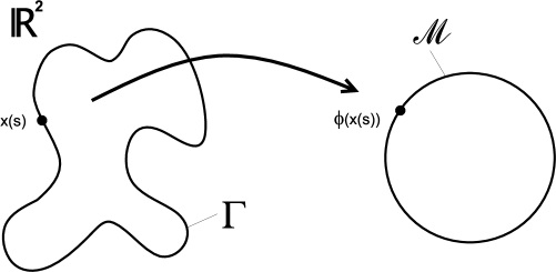
Figure 2: If the map indicated in this figure, $:\Gamma\rightarrow{\cal M}:{\bf x}(s)\mapsto\phi({\bf x}(s))$ is non-trivial, a cosmic string forms.

If we now leave the plane and continue this argument in the third dimension, we obtain a long, thin string within which $\phi$ assumes higher energy, a cosmic string. The cross section of the string, i.e. of the region where $\phi$ leaves the vacuum manifold, is typically of order $1/\eta$. The length of a string is either infinite or the string must be closed. The mechanism of defect formation described here is called the ’Kibble mechanism’ $\!{}^{{\bf?}}$.

The main ingredient for the Kibble mechanism is the existence non-trivial (non-shrinkable) maps from a closed curve is space $\sim{\bf S}^{1}$ to the vacuum manifold. The classes of these maps form a group, the first homotopy group $\Pi_{1}({\cal M})$.

Similarly, if maps from spheres in space into ${\cal M}$ cannot be shrunk to a point, i.e. $\Pi_{2}({\cal M})$ is non-trivial, $\phi$ might have to leave the vacuum manifold in a small patch in 3-space, leading to a tiny region of higher energy, a monopole. Again, the spatial extension of the monopole is on the order of $1/\eta$ and thus extremely small in comparison to cosmological scales.

Furthermore, if we consider configurations which are asymptotically constant ($\phi({\bf x})\rightarrow_{|{\bf x}|\rightarrow\infty}$ const.), we can compactify 3-space to $\overline{{\bf R}^{3}}=({\bf R}^{3}\cup\infty)\sim{\bf S}^{3}$, and assign to $\phi(\infty)$ the value of the asymptotic constant. We then encounter the question whether there exist non-shrinkable maps from ${\bf S}^{3}\rightarrow{\cal M}$. (Non-trivial homotopy group $\Pi_{3}({\cal M})$.) One can show, that such a configuration is always unstable and will shrink and eventually leave the vacuum manifold and unwind. (In the case of finite energy configurations this is Derrick’s theorem$\!{}^{{\bf?}}$.) A configuration $\phi$ which winds once around ${\bf S}^{3}$ is called ’texture’ of winding number 1. (Textures of higher winding numbers are probably unstable and decay into simple textures.)

There are some doubts about the applicability of this concept to cosmology; especially the notion of an asymptotically constant configuration is not at all causal. However, in the case of $\Pi_{3}$ (and only in this case!) one can define a texture number density $n_{\phi}(x)$, such that

$$w_{\phi}({\bf R}^{3})=\int_{{\bf R}^{3}}n_{\phi}(x)d^{3}x$$ (6)

determines the winding number (i.e. texture number) of the map $\phi:\overline{{\bf R}^{3}}\rightarrow{\cal M}$. Clearly, if this map is well defined, $w_{\phi}({\bf R}^{3})$ is always an integer. Nevertheless, we can also consider the winding number in a finite volume $V\in{\bf R}^{3}$ and determine

$$w_{\phi}(V)=\int_{V}n_{\phi}(x)d^{3}x$$ (7)

which need not be an integer. Numerical investigations$\!{}^{{\bf?}}$ have shown that a configuration shrinks whenever $w_{\phi}(V_{H})\stackrel{{\scriptstyle>}}{{\sim}}1/2$, where $V_{H}$ denotes the Hubble volume, independent of the behavior of $\phi$ at spatial infinity. Therefore, it makes sense to talk about textures also in a cosmological context.

Depending on whether the symmetry is local (gauged) or global (rigid), defects are called ’local’ or ’global’. In the case of local defects, gradients are compensated by the gauge potential ($\partial_{\mu}\rightarrow D_{\mu}=\partial_{\mu}+ieA_{\mu}$), and there is no considerable gradient energy. This has two important consequences:

• The energy of defects is strongly confined, i.e. the extension of defect energy is given by the inverse symmetry breaking scale, $1/\eta$.

• Soon after their formation, local defects cease to interact. There are no long range interactions between local defects.

In the case of global defects, there are no gauge fields to compensate gradients and the energy is dominated by gradient energy which is spread out over typically the horizon scale $t$. Interactions between defects are very strong. Defects of opposite charge annihilate leading to a few (or less) defects per horizon volume. Energy density always behaves like $\rho_{{\rm\small defect}}\sim\eta^{2}/t^{2}$ (up to possible logarithmic corrections) and we thus find $\rho_{{\rm\small defect}}/\rho_{{\rm\small matter}}\sim 4\pi G\eta^{2}=\epsilon$. The defect energy amounts to a constant small fraction of the total energy density of the universe. This behaviour is called scaling.

In the case of local defects, only strings scale. Local monopoles soon come to dominate the energy density of the universe and local textures quickly die out. Defects responsible for structure formation and CMB anisotropies are thus either local strings or global defects.

In the case of global fields, gradient energy is the main seed for perturbations in the geometry. Whether these gradients lead to topological defects or not is actually less important. E.g. scalar fields with a $\phi^{4}$ potential and $N>4$ components do not lead to topological defects in 3-dimensional space, but structure formation seeded by such fields is very similar to the $N=4$ (global texture) and $N=3$ (global monopoles) models. The limit $N\rightarrow\infty$ where the field equations can be solved exactly, provides a useful approximation to global defect scenarios $\!{}^{{\bf?},{\bf?}}$.

At temperatures significantly below the symmetry breaking scale, the dimensionless field $\beta=\phi/\eta$ obeys to a very good approximation the scale free equation of a non-linear $\sigma$–model $\!{}^{{\bf?}}$. Scaling arguments then yield ${\cal O}(\dot{\beta})={\cal O}(\partial_{i}\beta)={\cal O}(1/t)$.

The typical amplitude of geometrical fluctuations in scaling defect models is given by

$$4\pi G\rho_{{\rm\small defect}}/(\dot{a}/a)^{2}\sim 4\pi G\eta^{2}\equiv\epsilon~{}.$$ (8)

The COBE experiment provides the normalization $\epsilon\sim 10^{-5}$ and thus $\eta\sim 10^{16}$GeV. In order to create large enough fluctuation to seed the formation of structure in the universe, defects must thus form during a symmetry breaking phase transition at $T_{c}\sim 10^{16}$GeV, i.e. at a typical scale of grand unification.

3 The CMB Anisotropy Spectrum from Topological Defects

Anisotropies in the cosmic microwave background (CMB) are small and can thus be calculated within linear cosmological perturbation theory.

If we neglect the finite thickness of the last scattering surface, $t=t_{dec}$, the temperature anisotropies in the cosmic microwave background can be found by integrating photon geodesics from $t_{dec}$ until today, $t_{0}$. This leads to

$${\delta T\over T}({\bf n})=\left[{1\over 4}D^{(r)}+V_{j}n^{j}+(\Psi-\Phi)\right](t_{dec},{\bf x}_{dec})+\int_{i}^{f}(\dot{\Psi}-\dot{\Phi})({\bf x}^{\prime},t^{\prime})dt~{}.$$ (9)

Here $D^{(r)}$ denotes a gauge invariant variable describing intrinsic density fluctuations in the radiation, $\bf V$ is the peculiar baryon velocity, i.e. the velocity of the emitter (the corresponding term for the observer, which just results in the well-known dipole contribution has been omitted), and $\Phi$ and $\Psi$ are the Bardeen potentials$\!{}^{{\bf?}}$, two geometric variables which describe scalar perturbations of the Friedmann geometry. $\Psi$ is a close analog of the Newtonian potential. If the matter causing the geometric perturbation is either non-relativistic or an ideal fluid, $\Phi=-\Psi$. A derivation of Eq. (9) can be found in Ref. 12.

The first two terms in Eq. (9) are mainly caused by acoustic oscillations of the baryon photon fluid prior to recombination. This causal process acts only on sub horizon scales and thus comes to dominate on angular scales $\theta<1^{o}$. The third term is the ordinary Sachs Wolfe contribution$\!{}^{{\bf?}}$. It is due to the gravitational potential at the last scattering surface, which induces a redshift(blueshift) of the free photons climbing out of it (falling down from it). The integral in Eq. (9) is the integrated Sachs Wolfe term, which is induced by a time varying gravitational potential along the path of the photon from the last scattering surface into the antenna of the observer. The Sachs Wolfe contributions are relevant on large angular scales, $\theta\gg 1^{o}$.

The finite thickness of the last scattering surface leads to diffusion damping at very small angular scales: During recombination, the mean free path of photons grows from effectively $0$ to much larger than the Hubble scale. Perturbations with are small enough so that photons can diffuse out of them during the recombination process, are thus damped away. This process is called Silk damping$\!{}^{{\bf?}}$. To a reasonable approximation it can be taken into account by multiplying the result of Eq. (9) with an exponential damping envelope$\!{}^{{\bf?}}$. For a more accurate treatment, one has to solve Boltzmann’s equation taking into account non-relativistic Compton scattering of photons and electrons$\!{}^{{\bf?}}$.

In addition to these fluctuations which are determined entirely within linear perturbation theory, some secondary effects due to the formation of the first non-linear structures might influence the perturbations. There are notably gravitational lensing, the Rees Sciama effect and the Sunyaev Zel’dovich effect which can influence very small scales; as well as early reionization which may lead to damping of fluctuations on intermediate scales. Here we just discuss the Sachs Wolfe and acoustic contributions which dominate on large and intermediate angular scales.

Since ${\delta T\over T}$ is a function on the sphere, it make sense to expand it in terms of spherical harmonics:

$${\delta T\over T}({\bf n})=\sum_{\ell m}a_{\ell m}Y_{\ell m}({\bf n})~{}.$$ (10)

The anisotropy spectrum is then defined by

$$C_{\ell}={\langle\sum_{m}|a_{\ell m}|^{2}\rangle\over 2\ell+1}~{}.$$ (11)

In the case of Gaussian perturbations, the $C_{\ell}$’s contain the full statistical information of the CMB anisotropies since they are the ’harmonic transform’ of the two point correlation function:

$${\cal C}(\cos\vartheta)\equiv\left\langle{\delta T\over T}({\bf n}){\delta T\over T}({\bf n}^{\prime})\right\rangle\left|{}_{{~{}}_{\!\!({\bf n\cdot n}^{\prime}=\cos\vartheta)}}\right.={1\over 4\pi}\sum_{\ell}(2\ell+1)C_{\ell}P_{\ell}(\cos\vartheta)~{},$$ (12)

where $P_{\ell}$ denotes the Legendre polynomial of order $\ell$.

Since the relevant quantity for CMB anisotropies are the $C_{\ell}$’s, angular regimes are often translated into intervals of $\ell$’s. Small $\ell$’s probe large angular scales whereas large $\ell$’s probe small angular scales. The angular scale corresponding to a given $\ell$ is about $\theta_{\ell}\sim 1/\ell$. In terms of $\ell$, ’large angular scales’ correspond to $\ell\stackrel{{\scriptstyle<}}{{\sim}}50$ and Silk damping becomes relevant at $\ell\stackrel{{\scriptstyle>}}{{\sim}}800$. The scales in between are intermediate angular scales.

3.1 Large scales

Angular scales, $\theta\gg 1^{o}$, which correspond to spherical harmonics with index $\ell\ll 200$ subtend a distance which is larger than the size of the horizon at recombination. Temperature fluctuations on these angular scales are either due to super horizon fluctuations, if they result from fluctuations at the last scattering surface, the ’recombination shell’, or they have been induced during the propagation of the photons from the last scattering surface into the antenna of the observer.

The Sachs Wolfe (SW) contributions to the CMB anisotropies from inflationary models and defect models are as different as they can be. Nevertheless they finally lead to the same Harrison Zel’dovich spectrum of $C_{\ell}$’s. Let us elaborate on this ’accident’ in some detail.

For a pure CDM (cold dark matter) model, it is easy to show from the linear perturbation equations that $\Phi=-\Psi$ and $\dot{\Psi}=0.$ Furthermore, assuming adiabatic perturbations, one finds from the analog of Poisson’s equation, $(1/4)D^{(r)}=-(5/3)\Psi+{\cal O}((kt)^{2})$. On super horizon scales, $kt\ll 1$, Eq. (9) thus yields for pure CDM

$${\delta T\over T}({\bf n})={1\over 3}\Psi(t_{dec},{\bf x}_{dec})~{}.$$ (13)

This is the well known Sachs Wolfe result. For a typical inflationary spectrum, the Bardeen potentials behave like

$$\langle|\Psi(k)|^{2}\rangle\propto 1/k^{3}\mbox{ ~{}~{}~{}~{} for inflation + CDM.}$$ (14)

Using this and Eq. (13), one can calculate the anisotropy spectrum and finds (see appendix)

$$C_{\ell}\propto{1\over\ell(\ell+1)}~{}.$$ (15)

For topological defect models, the situation is very different. One can show, that (due to compensation) the Bardeen potentials have white noise spectra on super horizon sales $\!{}^{{\bf?},{\bf?}}$. By dimensional reasons therefore $\langle|\Psi(k)|^{2}\rangle t^{-3}=$constant. Furthermore, one finds that $D^{(r)}$ behaves like $(kt)^{2}\Psi$ and is thus negligible on super horizon scales. Once a perturbation enters the horizon, $t\sim 1/k$ the defect contribution decays and it is dominated by the contribution due to CDM which then becomes time independent. A reasonable approximation to the Bardeen potentials from defect models is thus

$$\langle|\Psi(k)|^{2}\rangle\propto\left\{\begin{array}[]{lll}t^{3},&\mbox{on super horizon scales,}&kt\leq 1,\\ 1/k^{3},&\mbox{on sub horizon scales,}&kt\geq 1,\end{array}\right.\mbox{ for defects + CDM.}$$ (16)

Using this approximation, it is easy to see that the ordinary Sachs Wolfe effect is very small (for scales which are super horizon at decoupling), whereas the integrated SW term behaves like the inflationary SW contribution leading to the same spectrum of CMB anisotropies on large angular scales, Eq (15). A derivation of this result is given in the appendix.

Of course, our argumentation in the case of topological defects is very crude. It is, however, useful to interpret the findings from numerical simulations. Large scale CMB anisotropies from simulations of Global defects$\!{}^{{\bf?}}$ are presented in Fig. 3. Similar results have been obtained for cosmic strings$\!{}^{{\bf?}}$.

Figure 3: The large scale CMB anisotropies from global texture simulations. The spectra for 27 observers are plotted. The sharp drop after $\ell\sim 30$ is due to finite resolution. (Figure taken from Durrer and Zhou, Ref. 17.)

3.2 Intermediate scales

The signal from CMB anisotropies on intermediate scales is most interesting since it contains the most structure and thus the most detailed information.

As already mentioned, fluctuations on intermediate scales are due to acoustic oscillations in the tightly coupled photon baryon plasma prior to recombination. To understand the basic principle, we treat these oscillations here in a very simple way. We neglect the presence of baryons and thus set the sound velocity of the plasma, $c_{s}^{2}=1/3$. Energy and momentum conservation then lead to the following equations of motion for the density perturbation $D^{(r)}$ and the peculiar velocity potential $V^{(r)}$ (see Ref. 12):

$$\dot{D}^{(r)}=-{4\over 3}kV^{(r)}~{}~{},~{}~{}~{}~{}\dot{V}^{(r)}=2k\Psi+{1\over 4}kD^{(r)}~{}.$$ (17)

(In the second equation we have suppressed the difference between $\Psi$ and $-\Phi$ which is unimportant for our qualitative discussion.) Eqs. (17) can be combined to a second order equation for $D$:

$$\ddot{D}^{(r)}+{1\over 3}k^{2}D^{(r)}=-{8\over 3}k^{2}\Psi~{}.$$ (18)

Using the behavior $\Psi\propto t^{3/2}$ on super horizon scales, and $\Psi\propto k^{-3/2}$ on sub horizon scales, we obtain the solutions

$$D^{(r)}=\left\{\begin{array}[]{lll}-{32\over 105}(kt)^{2}\Psi&\mbox{on super horizon scales,}&kt\ll 1\\ 8\Psi(\cos(kt/\sqrt{3})-1)&\mbox{on sub horizon scales,}&kt\gg 1.\end{array}\right.$$ (19)

This behavior of $D^{(r)}$ is very different to the adiabatic inflationary case. There $D^{(r)}\sim\Psi$ on super horizon scales and $D^{(r)}\sim\Psi(\sin(kt/\sqrt{3})-1)$ on sub horizon scales. For defects thus $D^{(r)}$ is very small at horizon crossing and first has to grow to achieve its maximum whereas in the adiabatic inflationary case, $D^{(r)}$ is already at its maximum on super horizon scales and starts decaying at horizon crossing. This is the reason why the first acoustic peak is displaced to larger $\ell$ for defect models. In a flat, $\Omega=1$ universe the position of the first acoustic peak is about $\ell_{peak}\sim 360$ for global defects where it is at $\ell=220$ for adiabatic inflationary models$\!{}^{{\bf?},{\bf?}}$.

I carefully always said ’adiabatic inflationary models’ since the second order Eq. (18) of course allows for two modes and in inflationary models one is actually free to choose the adiabatic mode, which is defined by $V^{(r)}=V^{(CDM)}$ on super horizon scales or the isocurvature mode which is defined by $D^{(r)}\rightarrow_{kt\rightarrow 0}0$. For defect models, however, we want to pick out the peculiar solution induced by the defect fluctuations without adding an arbitrary homogeneous solution, a perturbation which then would have to be induced by some other mechanism like, e.g. inflation. For defect models we thus have no freedom in the choice of the mode. The resulting CMB anisotropy spectrum for a typical model with global defects is shown in Fig. 4.

Figure 4: The CMB anisotropy spectrum from global topological defects. The vertical scale is arbitrary. This result was obtained by a model calculation as explained in Ref. 16.

An additional phenomenon which can be important for the acoustic peaks in the CMB anisotropy spectrum is decoherence: For inflationary perturbations the phase of an acoustic oscillation is entirely determined by its wave number, i.e. all fluctuations with fixed wave number $k$ are at fixed phase in their temporal oscillations. In models with topological defects, the fluctuations are induced by the defect energy which evolves in a complicated non-linear way. Decoherence can be described by the decay of the correlation function

$$C(k,t)={\langle|\Psi(k,t)\Psi(k,t_{i})|\rangle\over\sqrt{\langle|\Psi(k,t)|^{2}\rangle\langle|\Psi(k,t_{i})|^{2}\rangle}}~{}.$$ (20)

Since defects evolve causally, they are ’frozen in’ on super horizon scales and no decoherence can thus occur on these scales, $C(k,t)=1$, for $kt\ll 1$. As soon as defects enter the horizon, they start evolving in a complicated non-linear way and their gravitational potential looses coherence with a characteristic time scale $t_{c}$. On the other hand, the defects themselves decay with a decay time $t_{d}$. Once the defects have decayed, dark matter and radiation fluctuations evolve according to homogeneous perturbation equations not loosing any remaining coherence. The question whether decoherence is effective or not, is thus determined by the ratio $r=t_{c}/t_{d}$. For $r\leq 1$ decoherence is unimportant where as for $r\gg 1$ decoherence smears out secondary acoustic peaks leaving over just one broad ’hump’ $\!{}^{{\bf?}}$. This process is illustrated in Fig. 5.

Figure 5: CMB anisotropies from topological defects. The effect of decoherence is shown. The variables $\tau_{c}$ and $x_{c}$ correspond to $t_{d}$ and $t_{c}$ respectively. The ratio $r$ is thus largest for the top right frame and smallest for the bottom left one. (From Magueijo et al., Ref. 3.)

Local cosmic strings decay only via the very weak process of gravitational radiation and are thus relatively long lived. A cosmic string loop, after entering the horizon, typically survives for about $10^{4}$ horizon times. Global defects, on the other hand, decay very effectively within a few horizon times via the radiation of massless Goldstone modes. Furthermore, there are hints from numerical simulations, that coherence decays exponentially for cosmic strings$\!{}^{{\bf?}}$ but only like a power law for global defects$\!{}^{{\bf?}}$. These findings have led to the conjecture that decoherence is effective in scenarios with local cosmic strings but not for global defects. However, to fully understand and quantify decoherence, more detailed simulations and analytical work are needed.

4 Conclusion

We have seen that the anisotropies in the CMB provide interesting possibilities to distinguish between models of structure formation from inflationary perturbations or from topological defects. The first tests for physical theories at very high energies $\sim 10^{16}$GeV might thus come from cosmology and not from accelerator experiments!

One of the reasons for its usefulness certainly lies in the simplicity of calculations of CMB anisotropies. All the effects discussed here can be determined within linear perturbation analysis. The complicated non-linear physics involved in the formation of celestial bodies plays only a minor role for CMB anisotropies, while it might significantly obscure the relation between observations and calculations of large scale structure. There, the quantities simple to observe are the clustering properties of light, while linear perturbation analysis just determines the clustering of mass.

We have justified hopes that the next decade, when experimental results determine CMB anisotropy to an accuracy of a few percent, will revolutionize cosmology. On the one hand, the dependence of the details of the acoustic peaks on cosmological parameters$\!{}^{{\bf?}}$ might help us to determine these parameters to an accuracy of a few percent. On the other hand, the acoustic peaks probably contain information about the physics at GUT scales which is not available to us by any other means.

I have not discussed here the distinction of inflationary and defect models by statistical means: While generic inflationary models lead to Gaussian perturbations, topological defects are inherently non-Gaussian. It may however be quite difficult to detect this deviation from Gaussian statistics: On very large scales, a significant obstacle is cosmic variance, while on intermediate scales, several defects might contribute to a given perturbation and thus reduce non-Gaussian signatures (central limit theorem). The best prospects are probably on small scales, where one might actually ’see’ the discontinuity due to one cosmic string$\!{}^{{\bf?}}$. An interesting discussion of the problem of statistics is given in the contribution by J. Magueijo in these proceedings.

Appendix

In this appendix we show in some detail how Eqs. (14) and (16) lead both to a Harrison Zel’dovich spectrum of microwave background anisotropies, i.e. $C_{\ell}\propto 1/\ell(\ell+1)$.

Using ${\bf x}_{dec}={\bf x}_{0}-{\bf n}(t_{0}-t_{dec})\approx{\bf x}_{0}-{\bf n}t_{0}$, the Fourier transform of Eq. (13) yields

$${\delta T\over T}({\bf n,k})={1\over 3}\exp(i{\bf n\cdot k}t_{0})\Psi(t_{dec},{\bf k})~{}.$$ (21)

Using the well-known identity$\!{}^{{\bf?}}$ $\exp(i\alpha\mu)=\sum_{\ell}(2\ell+1)i^{\ell}j_{\ell}(\alpha)P_{\ell}(\mu)$, where $j_{\ell}$ denotes the spherical Bessel function and $P_{\ell}$ is the Legendre polynomial of index $\ell$, we find

$${\delta T\over T}(k,\mu)=\sum_{\ell}i^{\ell}\Delta_{\ell}(k)P_{\ell}(\mu)~{},$$ (22)

with $\mu={\bf n\cdot k}/k$, and

$$\Delta_{\ell}(k)={2\ell+1\over 3}\Psi(k,t_{dec})j_{\ell}(kt_{0})~{}.$$ (23)

Inserting this in the two point correlation function, Eq. (12), one obtains

$$C_{\ell}={2\over\pi}\int dkk^{2}{\langle|\Delta(k)|^{2}\rangle\over(2\ell+1)^{2}}~{}.$$ (24)

To arrive at this result we replace the ensemble average of Eq. (12) by an integration over observer positions ${\bf x}_{0}$, a kind of ’ergodic hypothesis’. Then we use unitarity of the Fourier transform and elementary orthogonality properties of spherical harmonics. The average $\langle|\Delta(k)|^{2}\rangle$ represents an integral over $\bf k$-directions. For Eq. (24) to hold, it is important that the Fourier transform is defined by

$$\hat{f}({\bf k})={1\over\sqrt{V}}\int_{V}d^{3}xf({\bf x})\exp(i{\bf k\cdot x})~{},$$ (25)

otherwise, the pre-factor in front of the integral in Eq. (24) changes.

Inserting now $\langle|\Psi|^{2}(k)\rangle=Ak^{-3}$, the integral in Eq (24) becomes

$$C_{\ell}={2A\over 9\pi}\int{dx\over x}j_{\ell}(x)^{2}~{}.$$

This integral can be performed exactly with the result$\!{}^{{\bf?}}$

$$C^{(inflation)}_{\ell}={A\Gamma(\ell)\over 36\Gamma(3/2)\Gamma(\ell+2)}={A\over 9\pi\ell(\ell+1)}~{}.$$ (26)

The dimensionless constant $A$ is given by the specific inflationary model and has to be tuned to $A\sim 10^{-9}$.

For topological defects the situation is somewhat more complicated since $\Psi$ is time dependent. The same reasoning which led to Eq. (23) yields

$${1\over 2\ell+1}\Delta_{\ell}(k)=2\Psi(t_{dec},k)j_{\ell}(kt_{0})+2\int_{t_{dec}}^{t_{0}}\dot{\Psi}(t,k)j_{\ell}(k(t_{0}-t))dt~{}.$$ (27)

If we now make use of the approximation for the geometry perturbations from defects given in Eq. (16) and simply set $\Psi({\bf k})\sim\sqrt{\langle|\Psi(k)|^{2}\rangle}$ , the integration in Eq. (27) has to be performed only until $t=1/k$, since $\dot{\Psi}$ vanishes for $kt>1$. We thus may neglect the weak time dependence of $j_{\ell}$ in the interval of integration. The integral in Eq. (27) can then be performed. The ordinary SW contribution is canceled by the lower limit of the integral and only the much larger contribution from the upper limit of the integral remains leading to

$$\Delta_{\ell}(k)=2(2\ell+1)\Psi(t=1/k,k)j_{\ell}(kt_{0})~{}.$$ (28)

Inserting this finding in Eq. (24) with $\langle|\Psi(t=1/k,k)|^{2}\rangle=A\epsilon^{2}k^{-3}$, we find as in Eq. (26)

$$C_{\ell}^{({\rm\small defect})}={8A\epsilon^{2}\over\pi\ell(\ell+1)}~{}.$$ (29)

Here $A$ is a dimensionless constant which is model dependent, but generically of order unity, and $\epsilon=4\pi G\eta^{2}$ is given by the symmetry breaking scale.

Even if the integration encountered in this derivation can be performed exactly, we should not forget that the crucial ingredient, Eq. (16) is a simple approximation and the constant $A$ should be determined by numerical simulations. Also in the simple inflationary CDM model, massless neutrini and the contribution of radiation to the expansion of the universe induce a small integrated SW contribution which has been neglected in this approximation.

In general, if $\langle|\Delta_{\ell}(k)|^{2}\rangle=Ak^{-n}t_{0}^{3-n}$ in a certain range of harmonics $\ell$, one can compute the $C_{\ell}$’s in this range exactly with the result

$$C_{\ell}=A{\Gamma(n-1)\Gamma(\ell+{3-n\over 2})\over 2^{n-1}\Gamma(n/2)^{2}\Gamma(\ell+{n+1\over 2})}~{}.$$

References

References

- [1] E. Lifshitz, J. Phys. USSR 10, 116 (1946).
-
[2]
E. Harrison, Phys. Rev. D1 2726 (1970);
Ya. B. Zel’dovich, Mont. Not. R. Astr. Soc. 160, P1 (1972). - [3] J. Magueijo, A. Albrecht, P. Ferreira and D. Coulson, Phys. Rev. D54, 3727 (1996).
- [4] J.I. Kapusta, “Finite Temperature Field Theory”, Cambridge University Press (1989).
- [5] T. W. B. Kibble, Phys. Rep. 67, 183 (1980).
- [6] J. Derrick, Math. Phys. 5, 1252 (1964).
- [7] J. Borill, E.J. Copeland, A.R. Liddle, A. Stebbins and S. Veeraraghavan, Phys. Rev. D50, 2469 (1994), and references therein.
- [8] N. Turok and D. Spergel, Phys. Rev. Lett. 66, 3093 (1991).
- [9] M. Kunz and R. Durrer, Phys Rev. D, in press, archived under astro-ph/9612202 (1996).
- [10] R. Durrer in: Formation and Interaction of Topological Defects, NATO ASI Series B349, eds. A.C. Davis and R. Brandenberger (1995).
- [11] J. Bardeen, Phys. Rev. D22, 1882 (1980).
- [12] R. Durrer, Fund. of Cosmic Physics 15, 209 (1994).
- [13] R.K. Sachs and A.M. Wolfe, Astrophys. J. 147, 73 (1967).
- [14] J. Silk, Astrophys. J. 151, 459 (1968).
- [15] W. Hu and N. Sugiyama, Astrophys. J. 471, 542 (1996).
- [16] R. Durrer and M. Sakellariadou, Phys. Rev. D, submitted, archived under astro-ph/9702028 (1997). (See also Sakellariadou & Durrer, these proceedings.)
- [17] R. Durrer and Z.H. Zhou Phys Rev. D53 (1995).
- [18] B. Allen, R.R. Caldwell, E.P.S. Shellard A. Stebbins and S. Veeraraghavan, Phys. Rev. Lett., submitted, archived under astro-ph/9609038 (1996)
- [19] R. Crittenden and N. Turok, Phys. Rev. Lett. 75, 2642 (1995).
- [20] R. Durrer, A. Gangui and M. Sakellariadou, Phys. Rev. Lett. 76, 579 (1996).
-
[21]
N. Kaiser and A. Stebbins, Nature 310, 391
(1984);
A. Stebbins Astrophys. J. 327, 584 (1988). - [22] W. Hu, N. Sugiyama and J. Silk, Nature, in press, archived under astro-ph/9604166 (1997).
- [23] M. Abramowitz and I.A. Stegun, Handbook of Mathematical Functions, Dover Publications, New York (1972).
- [24] I.S. Gradshteyn and I.M. Ryzhik, Tables of Integrals, Series and Products, Academic Press, San Diego (1980).