An Upper Limit to Arcminute Scale Anisotropy in the Cosmic Microwave Background Radiation at 142 GHz

Abstract

We present limits to anisotropies in the cosmic microwave background radiation (CMB) at angular scales of a few arcminutes. The observations were made at a frequency of 142 GHz using a 6-element bolometer array (the Sunyaev-Zel’dovich Infrared Experiment) at the Caltech Submillimeter Observatory. Two patches of sky, each approximately $36^{\prime}\times 4^{\prime}$ and free of known sources, were observed for a total of 6-8 hours each, resulting in approximately 80 independent $1\farcm 7$ full-width half-maximum pixels. Each pixel is observed with both a dual-beam and a triple-beam chop, with a sensitivity per pixel of 90-150 $\mu$K in each chop. These data have been analyzed using maximum likelihood techniques by assuming a gaussian autocorrelation function for the distribution of CMB fluctuations on the sky. We set an upper limit of $\Delta T/T\leq 2.1\times 10^{-5}$ (95% confidence) for a coherence angle to the fluctuations of $1\farcm 1$. These limits are comparable to the best limits obtained from centimeter-wavelength observations on similar angular scales but have the advantage that the contribution from known point sources is negligible at these frequencies. They are the most sensitive millimeter-wavelength limits for coherence angles $\leq 3^{\prime}$. The results are also considered in the context of secondary sources of anisotropy, specifically the Sunyaev-Zel’dovich effect from galaxy clusters.

1 Introduction

Measurements of anisotropies in the spatial distribution of the cosmic microwave background radiation (CMB) are a powerful probe of the early universe. In the standard inflationary model, anisotropies were imprinted on the CMB when the universe combined at $z\sim 1000$ (for a review of cosmological theories see, for example, White, Scott and Silk 1994). The attenuation of these primordial fluctuations in the CMB by the finite thickness of the surface of last scattering, and photon diffusion, suppress the anisotropy power spectrum at arcminute angular scales. The exact shape that is predicted for the power spectrum in this regime is strongly dependent on the assumed cosmological model. Additionally, an early period of re-ionization may have only a small effect on the anisotropy power spectrum at degree scales while strongly affecting the magnitude and shape of the power spectrum on arcminute scales. Thus measurements of, or upper limits on, the magnitude of the CMB power spectrum at arcminute scales are a powerful discriminant between competing models. Secondary sources of arcminute-scale anisotropies include the Sunyaev-Zel’dovich (S-Z) effect — the inverse Compton scattering of CMB photons by hot gas residing in the potential wells of galaxy clusters. Measurements at arcminute angular scales can provide important information for theories of large-scale structure formation via number counts of galaxy clusters with a measurable S-Z effect.

The Sunyaev-Zel’dovich Infrared Experiment (SuZIE) is a 6-element bolometer array that has been used to make the first detections of the S-Z effect at millimeter wavelengths (Wilbanks et al. (1994), Holzapfel et al. 1997a ). Coupled to the Caltech Submillimeter Observatory (CSO), this array has a sensitivity of 0.3 Jy/$\sqrt{\mbox{Hz}}$ at 142 GHz in each of six pixel pairs and angular resolution of $\sim 1\farcm 7$. This, and a scan strategy designed to minimize systematic effects, make it an ideal instrument with which to search for arcminute scale anisotropies in the CMB.

This paper describes observations made with the SuZIE receiver of two regions of sky that are free of known sources. The data are used to set limits on CMB fluctuations that are assumed to be distributed on the sky with a gaussian autocorrelation function (GACF). A companion paper (Ganga et al. 1997a ) considers the application of these results to specific cosmological models. In this paper we also consider the limits that these observations place on number counts of S-Z clusters.

2 The Instrument

The SuZIE bolometer array (described in detail in Holzapfel et al. 1997b ) is operated at the Caltech Submillimeter Observatory (CSO) on Mauna Kea. At 142 GHz, emission from the sky and the warm telescope optics are measured by SuZIE to contribute 36 K in brightness temperature. A tertiary mirror re-images the Cassegrain focus of the telescope to a focal plane comprising two rows of three bolometers cooled to 300 mK. Each bolometer is coupled to the primary mirror by a Winston concentrator that defines a $1\farcm 7$ full-width half-maximum (FWHM) beam on the sky. The two rows are separated by $2^{\prime}$, and adjacent pixels within a row by $2\farcm 3$. The illumination pattern of each Winston cone on the primary mirror is controlled by a 2 K Lyot stop located at an image of the primary produced by the tertiary mirror. To reduce systematic effects from spillover, only 8 m of the 10.4 m primary diameter are used.

SuZIE can be configured for operation at 142, 217 or 268 GHz by placing an appropriate metal-mesh band-pass filter in front of the Winston cones. The observations described here were made at 142 GHz with an 11% band-width filter. The spectral response of the instrument, in its telescope-ready configuration, was measured in the laboratory prior to the observations, including measurements that demonstrate negligible out-of-band leaks. The measured scatter of the band centers of all six channels about the mean value is less than 1.5% and that of the band-widths is less than 5%. The optical efficiency of each channel, including the effects of all filters, is measured to be 37%.

Electronic differencing between pixels in the same row is carried out to remove common-mode response to atmospheric and telescope emission. Two differences corresponding to 2$\farcm$3 on the sky and one to 4$\farcm$6 are obtained from each row of the array. This is accomplished by placing the two bolometers in an AC-biased bridge circuit (Wilbanks et al. (1990)), the output of which is synchronously demodulated to produce a stable DC signal corresponding to the brightness difference on the sky. In terms of atmospheric subtraction, this is equivalent to a square-wave chop on the sky at infinite frequency. High rejection ($>40\times$) of common-mode signals from detector temperature fluctuations and telescope and atmospheric emission (Glezer, Lange & Wilbanks (1992)) is achieved by trimming the amplitude of the bias voltage, and thus the responsivity of each detector. To ensure that the pixels that are being differenced are viewing the same column of atmosphere, and thus that maximum rejection of common-mode atmospheric fluctuations is obtained, the tertiary mirror is designed to maximize the overlap of the beams from the six Winston cones on the primary mirror without significantly degrading the focus. The illumination of the primary was measured at 217 GHz using a mobile 80 cm² load, and was verified to fall to $<-60$ db at a radius of 4.0 m from the primary center.

3 The Observations

SuZIE is designed to measure the S-Z effect in galaxy clusters. As part of this program, regions of sky free of known sources are observed to provide a check for baseline effects that might contaminate the S-Z measurements. We selected two such regions for observation in April 1994 at the positions listed in Table 1, using IRAS catalogs and the NRAO 5 GHz survey (Becker, White and Edwards (1991)) to avoid known sources. Each field is near a SuZIE target cluster, but at least 10 core radii away from the cluster center. The S-Z contribution to each pixel from any residual hot gas at this distance is $\Delta T_{\rm CMB}\leq 3$ $\mu$K, assuming an X-ray core radius of $1^{\prime}$, a $y$-parameter of $3\times 10^{-4}$ and, pessimistically, that the cluster gas is described by an isothermal, $\beta=2/3$, model out to many core radii (see for example Jones and Forman (1984)). Including the effects of differencing pixels in the focal plane will reduce this still further, depending on the angular scale on which the cluster gas is clumped.

In order to minimize systematic errors that might otherwise arise from position-dependent variations in telescope spillover, SuZIE observations are made by fixing the telescope position relative to the earth and allowing the source to drift across the array as the sky rotates. Each scan is two minutes long, yielding a $30^{\prime}\times\cos\delta$ strip of sky, where $\delta$ is the source declination. After each scan is completed, the dewar is rotated to keep the long axis of the array aligned in the direction of right ascension. The starting positions of successive scans alternate between $12^{\prime}$ and $18^{\prime}$ in RA ahead of the location listed in Table 1, providing a check for systematic effects that depend on position within a scan rather than on the pointing location of the telescope. Because there are two rows of detectors in the focal plane, the complete data set for a single field covers two strips of sky each $36^{\prime}\cos\delta$ in RA by $1\farcm 7$ in declination, with twice as much observing time allotted to the central two-thirds of each strip as for the outer portions. The observing scheme is summarized in Figure 1. Because both sources are close to the celestial equator, $\cos\delta\sim 1$ and the total area of sky covered is 0.057 square degrees.

4 Data Reduction and Calibration

Seven data sets were obtained, each corresponding to one night of observation on one field (typically 50-100 scans). Each data set is first split to separate the scans that correspond to the different RA offsets. The 6 differential measurements per data set that are obtained by electronically differencing each detector with other detectors in the same row are denoted by pairs $d_{pq}$ where $pq=$ 12, 23 and 31 for the first row and 45, 56 and 64 for the second row; the differential signal is the result of subtracting the $q$th from the $p$th detector voltage. The data were calibrated using drift-scan observations of Uranus for which the expected flux was calculated by convolving the spectral model for the source (Griffin and Orton (1993)) with the instrumental spectral response. The uncertainty in the absolute flux of Uranus at 142 GHz obtained by this method is $f_{\rm u}=\pm$6%. Corrections for atmospheric opacity due to the difference between the elevation of Uranus and the elevation of the Fields 1 and 2 observations were $<2$% (based on data from the CSO 225 GHz $\tau$-monitor extrapolated to 142 GHz). The result of the calibration is then a signal whose units are flux difference between the two beams. This is converted to $\Delta T_{\rm CMB}$ (the thermodynamic temperature difference between the two beams) as follows:

$$\Delta T_{\rm CMB}=\frac{\Delta I_{\rm CMB}}{I_{\rm CMB}}\frac{(e^{x}-1)}{xe^{x}}T_{\rm CMB}$$ (1)

where $x=h\nu/kT_{\rm CMB}$ and:

$$I_{\rm CMB}=\frac{2h\nu^{3}}{c^{2}}\frac{1}{(e^{x}-1)}\Omega_{\rm beam}$$ (2)

The temperature of the CMB is taken to be 2.726 K (Mather et al. (1994)); the effect of the 0.01 K uncertainty in $T_{\rm CMB}$ is negligible compared to other sources of calibration uncertainty.

The solid angle of one pixel, $\Omega_{\rm beam}$, is calculated from measurements of the beam profile made using Jupiter and Uranus. The 2-dimensional shape of the beam was determined from drift scans across Jupiter, with the array offset in declination from the source (transverse to the scan direction) by steps of $15^{\prime\prime}$. Jupiter is used for this measurement because it is very bright at 142 GHz and can thus be used to obtain high signal/noise measurements of the sidelobes and the aspect ratio of the beams. However, its large size ($40^{\prime\prime}$) compared to the SuZIE beam makes it unsuitable for a direct measurement of the beam solid angle. This is determined instead from drift scans across Uranus, by first assuming a circularly symmetric beam on the sky and integrating the beam profile and then correcting for the measured aspect ratio of the beams. Note that the beams are very nearly circular (see the Jupiter beam map in Holzapfel et al. 1997b ) with an aspect ratio (defined as FWHM in the scan direction divided by FWHM in the cross-scan direction) that varies from 0.94–1.13.

The uncertainty in the beam shapes, $f_{\rm b}$, (estimated from the scatter of the 6 measured solid angles about their mean value) contributes a further 5% to the calibration uncertainty. The total calibration uncertainty is then $f_{\rm c}=(f_{u}^{2}+f_{b}^{2})^{1/2}=8$% ($1\sigma$). This uncertainty is included in the likelihood analysis of the data carried out in §7.

Because each detector contributes to the signal measured by two pairs, the six data streams are not independent. To remove the degeneracy, the two $2\farcm 3$ pairs from each row are differenced to generate a double difference:

$$t_{123} = (d_{12}-d_{23})/2$$ (3)

$$t_{456} = (d_{45}-d_{56})/2$$ (4)

The data then comprise 4 independent differences, two single differences, $d_{31}$ and $d_{64}$, and two double differences, $t_{123}$ and $t_{456}$.

Cosmic ray impacts on the bolometers cause spikes in the data stream that must be removed. A point-by-point differentiation is carried out and spikes are identified by a large positive excursion followed by a large negative excursion, or vice versa. Approximately 5% of the data are removed by this process. The data are then binned by averaging together 15 samples (3 s of data), equivalent to a $0\farcm 75\cos\delta$ portion of the drift scan, thus oversampling the $1\farcm 7$ beam full-width half-maximum (FWHM) by a factor of $2.3/\!\cos\delta$.

A best fit offset and linear drift are removed from each scan prior to co-adding all scans. The linear drift arises from common-mode variations in signal, primarily from changes in the atmospheric or telescope temperature, that are not completely removed by differencing. The average values, and variance, of the removed linear drift for each chop are shown in Table 2. The effect of this process on the sensitivity of the system to CMB fluctuations is small, but is taken into account in the analysis in §7.

Because the residual noise is dominated by atmospheric emission fluctuations with a $1\!/\!f$-type spectrum (Holzapfel et al. 1997b ), the statistical error obtained at each point from the binning process is not a good estimate of the sensitivity of the system over longer integration times. The correlation time of the atmospheric noise can be estimated from the correlation functions of individual scans and is of order 5 s (defined as the time to the first zero in the correlation function). Consequently, the binned data points within a single scan are correlated over many bins. The effects of this correlation on the statistical properties of the data are considered further in §6.3. In order to assign a sensible weight to each scan, the rms scatter, $\sigma_{j}$, of the binned data in the $j$th scan about the best fit offset and linear gradient is taken to be a representative measure of the noise in that scan. If the atmospheric noise is normally-distributed within a scan and uncorrelated between scans, this is a good assumption. Note that this process also assumes that the contribution to the rms from true temperature anisotropies within a single scan is negligible. The implications of these various assumptions are discussed in §6.3.

The scans corresponding to a single RA offset observed on a single night are co-added by combining all of the data at the $i$th point in each scan to yield a signal $y_{i}$ with uncertainty $\sigma_{i}$ where:

$$y_{i} = \frac{\sum\limits_{j}y_{i,j}/\sigma_{j}^{2}}{\sum\limits_{j}1/\sigma_{j}^{2}}$$ (5)

$$\sigma_{i}^{2} = \frac{1}{\sum\limits_{j}1/\sigma_{j}^{2}}\hskip 28.45274pt.$$ (6)

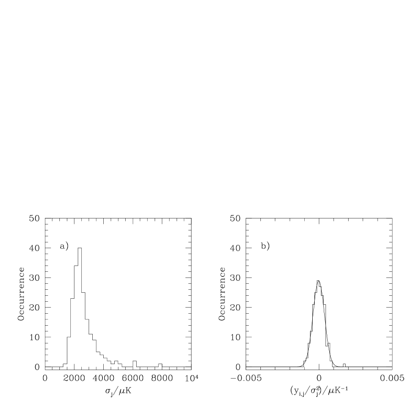
Figure 2: a) The distribution of the scan rms values, $\sigma_{j}$, for all 190 scans obtained on Field 1 with the $d_{64}$ difference. b) The distribution of the quantity $y_{i,j}/\sigma_{j}^{2}$ for a single bin from all 190 scans obtained on Field 1 with the $d_{64}$ difference. The solid line represents the normal distribution defined by the rms of $y_{i,j}/\sigma_{j}^{2}$ showing that this quantity is normally-distributed with no extreme values or large wings.

Here $\sigma_{j}$ is the rms of the $j$th scan after removal of the offset and linear drift, as described above. Note that $\sigma_{i}=\sigma$, a constant across the entire co-added scan. Figure 2a shows the distribution of the $\sigma_{j}$ values for Field 1 taken with the $d_{64}$ difference. Note that all of the data are included in the co-add and there is no cutting of data based on high values of scan rms, $\sigma_{j}$. Figure 2b shows the distribution of the quantity $y_{i,j}/\sigma_{j}^{2}$ evaluated for a single bin, again using all of the Field 1 scans and data corresponding to the $d_{64}$ difference. It can be seen that this quantity is normally-distributed with no extreme values or large wings. This indicates that the quantity $\sigma_{j}$ is a good estimate of the variance across the entire data set.

Co-added data from the two RA offsets are then combined by a weighted average of data points that correspond to the same position on the sky. Finally, a weighted average of the co-added data sets from each night is carried out. Figure 3 shows the final co-added data set for Field 1. The rms uncertainty for each $0\farcm 75$ bin is 130–220 $\mu$K, corresponding to a sensitivity of 3–5 mK s^1/2 for each difference. Both of the single and double difference data sets are shown, with the appropriate beam response to a point source (measured by drift scans across Uranus) indicated in each panel. Approximately 6 hrs of integration time (190 scans) were obtained on Field 1 and 9 hrs (277 scans) on Field 2. Note that double differencing reduces the error bars associated with the $t_{123}$ data points relative to those of $d_{31}$ in Figure 3, as residual atmospheric gradients are being removed from the data. In the case of $t_{456}$ and $d_{64}$, no such improvement is seen, probably due to poor common mode rejection in one of the two pairs that are combined to form $t_{456}$.

5 Statistical Analysis of the Data

The data are first examined without prejudice as to the origin of any possible excess signal by performing a series of statistical tests on each data set.

The simplest test that can be performed on the data is a calculation of the value of $\chi^{2}$ for each chop and each field, the results of which are shown in Table 3. All chops have values of $\chi^{2}$ that lie within the 95% ($\sim 2\sigma$) probability range for 46 degrees of freedom. However there appears to be a systematic bias towards $\chi^{2}$ values less than 46, indicating that the diagonal correlation assumption is incorrect. This is the effect of the residual correlation across the co-added data introduced by the presence of atmospheric $1\!/\!f$ noise. The implications of this correlation are considered further is §6.3.

A maximum likelihood analysis (Lawrence et al. (1988)) has been carried out on each data set to determine the most likely amplitude for any excess variance above the noise term described by the uncertainties, $\sigma_{i}$. For simplicity, we assume that all points within a single data set are independent, ignoring the correlation between adjacent data points that is introduced by smearing of any true CMB signal by the beams, or by the presence of $1\!/\!f$ noise in the data.

Each data set is analyzed separately using a maximum likelihood estimator with the likelihood of an excess variance of $\sigma_{e}^{2}$ being:

$$L(\sigma_{e})=\prod\limits_{i=1}^{N}\frac{1}{[2\pi(\sigma_{i}^{2}+\sigma_{e}^{2})]^{1/2}}\exp\left[\frac{-y^{2}_{i}}{2(\sigma_{i}^{2}+\sigma_{e}^{2})}\right]$$ (7)

The normalized likelihood as a function of $\sigma_{e}$ for each difference within each field is shown in Figure 4. There is no data set for which $\sigma_{e}\neq 0$ is significantly more likely than $\sigma_{e}=0$, as expected from the $\chi^{2}$ analysis. To determine limits on $\sigma_{e}$ from these curves, we adopt a Bayesian approach with a suitable choice of prior. For consistency with experiments that span a similar range of angular scales (e.g. Myers et al. (1993)) we adopt a prior that is uniform in $\sigma_{e}$. The 95% ($\sigma_{95}\sim 2\sigma$) and 99.7% ($\sigma_{99.7}\sim 3\sigma$) limits are then calculated using the highest probability density method (HPD, Berger (1985)), in which

$$I=100\times\frac{\int_{\sigma_{l}}^{\sigma_{u}}L(\sigma_{e})\,{\rm d}\sigma_{e}}{\int_{0}^{\infty}L(\sigma_{e})d\sigma_{e}},$$ (8)

with the constraint that $L(\sigma_{l})=L(\sigma_{u})$, yields $I=$ 95 or 99.7%. The values $\sigma_{l}$ and $\sigma_{u}$ are the lower and upper confidence limits respectively. The 95% and 99.7% confidence limits to $\sigma_{l}$ are zero for all of the data sets presented here. The 95% and 99.7% confidence limits for $\sigma_{u}$ are summarized in Table 4. The position of the likelihood peak is also indicated.

We now examine the validity of the assumption that any excess variance is uncorrelated across the data set. The autocorrelation function of the data, $C_{r}$, defined as:

$$C_{r} = \langle y_{i}\,y_{i+r}\rangle$$ (9)

$$= \frac{\sum\limits_{i=1}^{N-r}(y_{i}/\sigma_{i}^{2})(y_{i+r}/\sigma_{i+r}^{2})}{\sum\limits_{i=1}^{N-r}1/(\sigma_{i}^{2}\,\sigma_{i+r}^{2})}$$ (10)

(where $y_{i}$ and $\sigma_{i}$ are defined in equations 5 and 6) with an associated uncertainty, $\sigma_{C,r}$, given by:

$$\sigma^{2}_{C,r}=\frac{1}{\sum\limits_{i=1}^{N-r}1/(\sigma_{i}^{2}\,\sigma_{i+r}^{2})}$$ (11)

is shown in Figure 5 for data from Field 2. Significant structure can be seen in some of the differences. Possible non-astronomical sources for this structure are now considered.

6 Limits on Systematic Effects in the Data Sets

6.1 Systematic effects correlated with scan time

The standard SuZIE observing mode, in which the starting RAs of drift scans are alternately 12^′ and 18^′ in RA ahead of the nominal source position (see Figure 1), allows checks for systematics that are a function of time within a scan rather than pointing location on the sky. To check for such effects, the cross-correlation of the co-added data corresponding to the 12^′ offset with the co-added data corresponding to the 18^′ offset has been calculated for each chop. Artifacts that occur at the same time after the beginning of a scan will be seen in the cross-correlation function as a peak at zero time-lag. True astronomical signals in the data will yield a feature in the correlation function at a lag of $\Delta t=-4\Delta\theta\cos\delta$ where $\Delta\theta=6^{\prime}$ and $\delta$ is the source declination. Since both fields are close to the celestial equator $\Delta t\approx-24$ s.

Figure 6 shows the cross-correlation of data from the two offsets for data sets corresponding to Field 2. None of the chops show any strong features at zero lag, indicating that there are no systematic effects in the data that occur at the same time after the beginning of a scan. Peaks in the correlation functions at $\Delta t\neq 0$ are seen, but there are no peaks at $\Delta t=-24$ s that would indicate the presence of true astronomical signal (the peak in $t_{456}$ is at $-30$ s and is not repeated in any other chop). The most likely cause of these peaks is chance correlation of low-frequency $1\!/\!f$ noise which, in this experiment, is dominated by atmospheric emission fluctuations (see §6.3). The long ($\sim 5$ s) coherence time of atmospheric emission fluctuations correlates data at the end of one scan with the data at the start of the next. The telescope moves by about $30^{\prime}$ between scans, corresponding to a change in position of the beams of $<8$ m at heights $<1$ km above the telescope. This is less than the correlation length of atmospheric structure which is $\sim 25$ m (assuming a wind speed of 5 ms^-1 and a measured correlation time of order 5 s). Co-adding many scans will reduce the magnitude of this correlation but will not eliminate it entirely. This effect manifests itself in the cross-correlation functions shown in Figure 6 as non-zero correlations observed at time lags of $\pm 120$ s.

6.2 Cold stage temperature drifts

During SuZIE observations, the telescope is stationary during a scan, then re-acquires the source before the next scan begins. The motion of the telescope between scans results in a small excursion in the temperature of the 300 mK stage at the start of a new scan. The output of the temperature sensor on the 300 mK stage, co-added in the same way as the science data, is shown in Figure 7. The amplitude of the temperature excursion at the beginning of the scan is $\sim 80$ nK. The temperature recovers with a time constant of $\sim$ 10 s, and is stable to $\sim$ 10 nK rms for the duration of the scan.

Although the excursion at the beginning of each scan is very small, we have carried out a number of checks to determine whether this temperature drift causes residual artifacts in the co-added data sets. First, as described in §6.1, such an artifact would be seen as a peak at zero lag in the cross-correlations of data from the two RA offsets, shown in Figure 6. No significant peak is seen. Second, since the temperature sensor data is sampled at an identical rate to the science data, the measured temperature drift can be correlated with the science channels on a scan-by-scan basis. The maximum correlated change in signal in the science channels is $\Delta T_{\rm CMB}<4$ $\mu$K, well below other sources of noise.

This analysis assumes that the shape and the phase of any temperature change in the science channels is identical to that observed in the temperature sensor. Because of differences in the thermal properties of the sensor and the bolometers, this may not be true. Consequently, there could be a large residual effect in the science data that is poorly correlated to the sensor data. As a final check, new co-added data sets were generated after excluding the first 21 s (7 bins) of data from each scan, and the likelihood analysis in §5 repeated. As shown in Figure 8, the sole effect on the calculated likelihood is an increase in the confidence limits caused by the effective reduction in integration time.

From these various tests, we conclude that any signal in the data caused by drifts in the temperature of the 300 mK stage is much smaller than the experimental uncertainties and can be ignored.

6.3 Atmospheric effects

Fluctuations in atmospheric emission, caused predominantly by variations in water vapor content, contribute $1\!/\!f$ noise to the data with a typical correlation time of 5 s, significantly less than the scan length. We therefore assume that data corresponding to the same coordinates on the sky but separated in time by more than one scan are uncorrelated (this assumption ignores the correlation of data at the end of one scan with data at the beginning of the next that causes correlations on angular scales of $24^{\prime}$ and $36^{\prime}$ in the full co-added data sets; we assume that the effects of atmospheric noise correlated between scans are small). This assumption allows an estimate of the residual contribution to the correlation function of the co-added data.

Representing the $i$th data point in the $j$th scan by the sum of $t_{i}$, the true astronomical signal that remains unchanged between scans, and $n_{i,j}$, the noisy signal from all sources for which the coherence time is less than the scan length, the correlation function of the co-added signal is then:

$$S_{r}={\cal C}_{r}+{\cal N}_{r}$$ (12)

Here ${\cal C}_{r}=\langle t_{i}\,t_{i+r}\rangle$ is the correlation function of the true astronomical signal and ${\cal N}_{r}$ is the residual correlation function of the noisy part of the signal. It can be shown (Appendix A) that ${\cal N}_{r}$ is given by:

$${\cal N}_{r}=\frac{\sum\limits_{j}{\cal N}_{r,j}/\sigma^{4}_{j}}{(\sum\limits_{j}1/\sigma^{2}_{j})^{2}}$$ (13)

where ${\cal N}_{r,j}$ is the correlation function of $n_{i,j}$ in the $j$th scan. This expression can be rewritten as:

$${\cal N}_{r}=\left(\frac{\sum\limits_{j}{\cal N}_{r,j}/\sigma^{4}_{j}}{\sum\limits_{j}1/\sigma^{4}_{j}}\right)\times\left[\frac{\sum\limits_{j}1/\sigma^{4}_{j}}{(\sum\limits_{j}1/\sigma^{2}_{j})^{2}}\right]$$ (14)

where the first term is the correlation function of the atmospheric noise in a single scan averaged over all scans, and the second term is equal to $1/N$ if the uncertainty, $\sigma_{j}$, is roughly constant over all scans. Since the correlation function of a single scan is given by:

$$S_{r,j} = \langle(t_{i}+n_{i,j})(t_{i+r}+n_{i+r,j})\rangle$$ (15)

$$= {\cal C}_{r}+{\cal N}_{r,j}$$ (16)

it is clearly not possible to calculate ${\cal N}_{r,j}$ independently of the contribution from the true astronomical correlation function. However, if we assume that the atmospheric noise within the individual scans dominates the true astronomical signal in each scan then ${\cal N}_{r,j}\sim S_{r,j}$ and the estimated residual correlation function from atmospheric noise, ${\cal N}^{e}_{r}$, can then be calculated using Equation 13 with ${\cal N}_{r,j}=S_{r,j}$. Note that ${\cal N}_{r,j}\gg{\cal C}_{r}$ is implicit in the assumption made in §4, Equations 5 and 6, that the uncertainty, $\sigma_{i,j}$, associated with the data points in an individual scan is equal to $\sigma_{j}$, the rms of an entire scan.

How valid is this assumption? Since the residual atmospheric noise calculated using Equation 13 is approximately equal to the average correlation function per scan divided by the total number of scans, the contribution of the true astronomical correlation function, ${\cal C}_{r}$, to ${\cal N}^{e}_{r}$ calculated using Equation 13 is $\sim{\cal C}_{r}/N$. Since N is typically 100 per RA offset for each field, this contribution is clearly very small compared to ${\cal C}_{r}$. Therefore, if the calculated function, ${\cal N}^{e}_{r}$, is compared with the measured correlation function of the co-added data there are several possibilities: (i) if ${\cal N}_{r,j}$ and ${\cal N}_{r}\gg{\cal C}_{r}$ then the contribution of ${\cal C}_{r}$ to ${\cal N}^{e}_{r}$ will be negligible and ${\cal N}^{e}_{r}$ will be a good fit to the correlation functions shown in Figure 5; (ii) if ${\cal N}_{r,j}$ and ${\cal N}_{r}\ll{\cal C}_{r}$ then the calculated function ${\cal N}^{e}_{r}$ will be $\sim{\cal C}_{r}/N$. Thus ${\cal N}^{e}_{r}$ will have the right shape, but will have an amplitude that is too low by approximately two orders of magnitude; (iii) if ${\cal N}_{r}$ and ${\cal C}_{r}$ have comparable magnitudes then ${\cal N}^{e}_{r}$ will be a poor fit to the measured correlation functions.

Figure 9 shows the estimated correlation function of the residual atmospheric noise, ${\cal N}^{e}_{r}$, calculated using the methods given above, overlaid on the correlation function of the co-added data corresponding to one RA offset taken from Field 1. At angles less than $10^{\prime}$, the correlation function of the co-added data is moderately well fitted by ${\cal N}^{e}_{r}$, corresponding to case (i) above and indicating that the majority of the observed correlation in the data on these scales is due to atmospheric noise or other sources of $1\!/\!f$ noise. There are some large deviations however, particularly in the data from row 2 (pixels 4, 5 and 6). Since this row is known to be more susceptible than row 1 to atmospheric fluctuations, these large correlations are likely to be the result of atmospheric drifts that are correlated on time scales longer than one scan (see §6.1).

7 Comparison of the Data with Gaussian Models of CMB Anisotropies

In order to compare the data to specific models for the power spectrum of CMB fluctuations, the correlation properties introduced by the beam response on the sky, and the overlap on the sky of the single and double differences, must be taken into account. We represent the correlation function of true temperature anisotropies by:

$${\cal C}_{r}=C({\bf n}_{a}{\bf n}_{b})=\langle T({\bf n}_{a})T({\bf n}_{b})\rangle$$ (17)

where ${\bf n}_{a}$ and ${\bf n}_{b}$ are directions on the sky. If the CMB sky is assumed to be sampled from a gaussian random field then $C({\bf n}_{a}\,{\bf n}_{b})$ can be written as $\Delta T_{0}^{2}\times{\cal F}(\theta)$ where the spatial dependence of the function ${\cal F}(\theta)$ depends only the angular separation, $\theta$, between the two vectors ${\bf n}_{a}$ and ${\bf n}_{b}$. The model correlation function, $\overline{C}_{r}$, of the measured data in the absence of any noise sources is then given by:

$${\cal C}_{r}=\overline{C}_{r}=\langle\overline{T}_{i}\,\overline{T}_{i+r}\rangle=\Delta T_{0}^{2}\times\overline{\cal F}(r\Delta\theta)$$ (18)

where $\overline{T}_{i}$ and $\overline{T}_{i+r}$ are the predicted thermodynamic temperatures of pixels $i$ and $i+r$ in the data stream after convolution of the true temperatures with the beam of the instrument. The quantity $\Delta\theta$ is the sampling rate on the sky. For instance, the correlation function between data points measured in the single difference data set, $d_{31}$, is given by:

$$\langle\overline{T}_{i}\,\overline{T}_{i+r}\rangle_{31}=\int\limits_{{\bf n}_{a}}\int\limits_{{\bf n}_{b}}\langle T({\bf n}_{a})\,T({\bf n}_{b})\rangle\ [A_{3}({\bf n}_{i}-{\bf n}_{a})-A_{1}({\bf n}_{i}-{\bf n}_{a})]\ [A_{3}({\bf n}_{i+r}-{\bf n}_{b})-A_{1}({\bf n}_{i+r}-{\bf n}_{b})]\ {\rm d}{\bf n}_{a}{\rm d}{\bf n}_{b}$$ (19)

where $A_{j}$ is the beam response function of pixel $j$ in the SuZIE array.

A simultaneous likelihood analysis for all data from one field can be performed by combining all four differences into one data vector ${\bf y}$ of length $4N$, where $N$ is the number of 45^′′ data bins. The likelihood of the model correlation function, given the data, can be calculated as follows:

$$L(\Delta T_{0},{\cal F})=\frac{1}{(2\pi)^{N/2}|{\bf M}|^{1/2}}\exp(-{\bf y}^{T}{\bf M}^{-1}\,{\bf y})$$ (20)

The $4N\times 4N$ matrix ${\bf M}$ is composed of sub-matrices ${\bf m}^{pq}$ where $p,q=1,4$. The elements of each sub-matrix are given by:

$$m^{pq}_{i,j}=\overline{C}^{pq}_{j-i}+{\cal N}^{pq}_{j-i}$$ (21)

where $i,j=1,N$. The function $\overline{C}^{pq}_{j-i}$ is given by Equation 19 with the beam responses for the appropriate differences inserted. The function ${\cal N}^{pq}_{j-i}$ is the correlation function of the noise component to the data.

We need, however, to account for the loss of degrees of freedom introduced by the removal of a mean and linear drift from each scan. The process, adapted from Bond et al. (1991), is summarized here. The true CMB signal that has been subtracted from the data by the removal of an offset and linear drift can be represented as an unknown amount, ${\bf a}$, of a set of fitting functions, ${\bf F}$. The data vector, ${\bf y}$, can be corrected for this process by defining a vector ${\bf y}_{\rm true}$ such that:

$${\bf y}={\bf y}_{\rm true}-{\bf a}^{T}{\bf F}$$ (22)

The unknown vector ${\bf a}^{T}$ has length 8 (the product of the number of differences and two fitting functions); ${\bf F}$ is a known $8\times 4N$ matrix with elements equal to the value of the fitting functions ($F_{i,j}=1$ for $i=1,3,5,7$ is the basis function for the offset, and $F_{i,j}=j$ modulo $N$ for $i=2,4,6,8$ is the basis function for the slope, where $j=1,4N$). Thus the likelihood function in Equation 20 should be written as:

$$L(\Delta T_{0},{\cal F})=\frac{1}{(2\pi)^{N/2}|{\bf M}|^{1/2}}\exp[-({\bf y}+{\bf a}{\bf F})^{T}{\bf M}^{-1}\,({\bf y}+{\bf a}{\bf F})]$$ (23)

Assuming a uniform prior for, and integrating over, the unknown vector ${\bf a}$ yields:

$$L_{\rm new}(\Delta T_{0},{\cal F})\propto\frac{1}{(|{\bf M}||{\bf F}^{T}{\bf M}^{-1}{\bf F}|)^{1/2}}\exp\left[\frac{-{\bf y}^{T}{\bf M}^{-1}{\bf y}+{\bf y}^{T}{\bf M}^{-1}{\bf F}({\bf F}^{T}{\bf M}^{-1}{\bf F})^{-1}{\bf F}^{T}({\bf M}^{-1})^{T}{\bf y}}{2}\right]$$ (24)

Extending this analysis to include data from both fields is quite simple since the two patches of sky are widely separated on the sky, and also widely separated in terms of observing time. Thus the two data sets are completely uncorrelated both spatially and temporally and the matrix ${\bf M}$ for the complete data set is:

$${\bf M}_{\rm tot}=\left(\begin{array}[]{cc}{\bf M}_{1}&0\\ 0&{\bf M}_{2}\\ \end{array}\right)$$ (25)

The likelihood function for all data from both fields is then:

$$L_{\rm tot}=L_{1}\times L_{2}$$ (26)

where $L_{1}$ and $L_{2}$ are calculated from Equation 24. The calibration uncertainty is included at this point in the following manner. The measured amplitude of the sky correlation function, $\Delta T^{\prime}_{0}$ is assumed to be related to the true value $\Delta T_{0}$ by $\Delta T^{\prime}_{0}=G\times\Delta T_{0}$, where G is gaussian-distributed with width $\sigma_{G}$ (the fractional calibration uncertainty). It can then be shown (Ganga et al. 1997b ) that the likelihood of the true amplitude is obtained from the likelihood of the measured amplitude by:

$$L(\Delta T_{0},{\cal F})=\frac{1}{\sqrt{2\pi}\,\sigma_{G}\,\Delta T_{0}}\times\int\limits_{0}^{\infty}d(\Delta T^{\prime}_{0})\exp\left[\frac{-(\Delta T^{\prime}_{0}-\Delta T_{0})^{2}}{2\sigma_{G}^{2}\Delta T_{0}}\right]L(\Delta T^{\prime}_{0},{\cal F})$$ (27)

There remains the issue of the noise term ${\cal N}^{pq}_{j-i}$ in Equation 21. The simplest assumption is that the noise terms are uncorrelated between separate pixels and differences and that ${\cal N}^{pq}_{j-i}=\delta(p-q,j-i)\times(\sigma^{p}_{i})^{2}$ where $\sigma_{i}^{p}$ is the uncertainty associated with the $i$th data point in difference $p$. However, as shown in §6.3, there is a significant component of $1\!/\!f$ noise in the data that introduces correlations between pixels and also between the different chops. In principle, the non-diagonal noise terms can be estimated using Equation 13. However, this will not account for the residual features in Figure 9 that are believed to be caused by slow drifts correlated across more than one scan, and that are not well fitted by Equation 13.

Instead we adopt the following approach. Because ${\cal N}^{e}_{r}$ is such a good fit to the correlation function of the co-added data, there is unlikely to be a high signal/noise detection of astronomical signal. Thus the data can be analyzed assuming the simple $\delta$-function form for ${\cal N}^{pq}_{j-i}$ with the constraint that the results from the likelihood analysis should be treated as upper limits only to any signal in the data. The possible effects of ignoring the correlated noise component are discussed in §7.1.

To summarize, the elements of the sub-matrices ${\bf m}^{pq}$ are $m^{pq}_{i,j}=\overline{C}^{pq}(r\Delta\theta)+\mbox{$\delta(p-q,r)$}\,(\sigma_{p})^{2}$ where $r=j-i$ and $\Delta\theta=0\farcm 75\times\cos\delta$ is the sampling interval of the data on the sky. The modified correlation function, ${\overline{C}}^{pq}(r\Delta\theta)$ is obtained from Equation 19.

7.1 Comparison With a Gaussian Autocorrelation Function

The generalized form for $C(\theta)$ is an expansion in terms of Legendre polynomials, $P_{l}(\cos\theta)$:

$$C(\theta)=\frac{1}{4\pi}\sum\limits_{l=2}^{\infty}(2l+1)C_{l}P_{l}(\cos\theta)$$ (28)

where the function $C_{l}$ depends on the assumed cosmological model. The functional form of $C_{l}$ due to anisotropies imprinted at recombination has been extensively modeled in the literature (White et al. (1994), Bunn and Sugiyama (1995), Górski et al. (1995), Ratra et al. (1997)) and the implications of the SuZIE measurements for these models are considered in a companion paper (Ganga et al. 1997a ). In this paper we consider our measurements in terms of secondary sources of anisotropy from a population of S-Z clusters, since these may be comparable to, or larger than, primary anisotropies at these angular scales (Bond (1995)). The analytically simple gaussian autocorrelation function (GACF) model for $C(\theta)$, while a poor approximation to the power spectrum of primordial anisotropies, is a useful tool in this case.

The functional forms for the GACF is:

$$C(\theta)=C_{0}\exp\left[\frac{-\theta^{2}}{2\theta_{0}^{2}}\right]\\$$ (29)

with two free parameters, $C_{0}=\Delta T^{2}_{0}$, the variance, and $\theta_{0}$, the coherence angle, of the fluctuations. In the absence of other noise sources, observations of anisotropies distributed with this correlation function, using a gaussian beam of FWHM $\theta_{b}$, yield measurements with correlation function:

$$\overline{C}(\theta)=\frac{C_{0}\theta_{0}^{2}}{2\beta^{2}+\theta_{0}^{2}}\exp\left[\frac{-\theta^{2}}{2(2\beta^{2}+\theta_{0}^{2})}\right]$$ (30)

where $\beta=\theta_{b}/\sqrt{8\log 2}$.

The SuZIE beams are assumed to be gaussian, with a FWHM of 1$\farcm$7, derived by normalization to the measured solid angle. If a gaussian is fitted directly to the beam profiles, then the derived FWHM is 6% larger, however, this gaussian overestimates the beam shape at several beam widths away from the beam center. The 6% difference can be taken as some measure of the uncertainty that is introduced by assuming a gaussian beam. Ganga et al. (1997b) show that beam uncertainties of this magnitude do not affect the results of the modeling although they must be included in the calibration uncertainty, as we have done in §4.

The likelihood contours as a function of $(C_{0})^{1/2}$ and coherence angle, $\theta_{0}$, from a simultaneous likelihood analysis of all data from all fields, are shown in Figure 10a. A peak in the likelihood function at non-zero values of $C_{0}\neq 0$ is obtained for all coherence angles less than $10^{\prime}$. Using the HPD method with a uniform prior in $(C_{0})^{1/2}$, the 68%, 95% and 99.7% confidence limits on $(C_{0})^{1/2}$ for each value of $\theta_{0}$ have been calculated, and are shown in Figure 10b. The peak in the likelihood function has low significant ($\leq$ 68% confidence) and is consistent with noise. Consequently we confine ourselves to considering the 95% and 99.7% confidence limits. The coherence angle at which maximum sensitivity to $C_{0}$ is obtained is $\theta_{0}=1\farcm 1$; at this coherence angle, $(C_{0})^{1/2}\leq$ 58 $\mu$K (95% confidence) and $\leq$ 72 $\mu$K (99.7% confidence). Expressing these limits in terms of $\Delta T/T$ yields:

$$\Delta T/T\leq\left\{\begin{array}[]{ll}2.1\times 10^{-5}\mbox{\hskip 14.22636pt (95\% confidence)}\\ 2.6\times 10^{-5}\mbox{\hskip 14.22636pt (99.7\% confidence)}\end{array}\right.$$ (31)

These limits have been calculated without including the correlated terms in the matrix M that are introduced by the presence of atmospheric noise in the data. As such we believe the limits to be conservative. To check this assumption, we have re-analyzed just the data corresponding to the $d_{31}$ and $d_{64}$ chops, at the coherence angle of maximum sensitivity ($\theta_{0}=1\farcm 1$) only, with the inclusion of the terms ${\cal N}^{pq}_{j-i}$ in Equation 21. These terms have been calculated as outlined in §6.3. Ignoring data from the triple beam differences, $t_{123}$ and $t_{456}$, does not significantly degrade the derived upper limits. We find that the limits that are derived when the correlated noise terms are included are somewhat lower than those calculated when the correlated terms are ignored. Consequently the assumption that our upper limits are conservative is valid.

It is also useful to express these limits in terms of $\overline{C}(0)=C_{0}\theta_{0}^{2}/(2\beta^{2}+\theta_{0}^{2})$, the variance of sky fluctuations described by a GACF after convolution with a single gaussian beam. The most likely value, and the 95% and 99.7% limits, for ${\Delta}T_{\rm rms}=[\overline{C}(0)]^{1/2}$ are shown in Figure 11. At small values of $\theta_{0}$, our experiment is unable to distinguish between GACFs with different coherence angles and so $\Delta T_{\rm rms}$ tends towards a constant value as $\theta_{0}$ tends to zero. At large values of $\theta_{0}$, the SuZIE differencing scheme decreases the sensitivity to ${\Delta}T_{\rm rms}$ and so the limits rise steeply with increasing $\theta_{0}$. Selecting the value of $\theta_{0}=1\farcm 1$ (the GACF to which this experiment is most sensitive) yields upper limits on ${\Delta}T_{\rm rms}$ of:

$$\Delta T_{\rm rms}/T\leq\left\{\begin{array}[]{ll}1.6\times 10^{-5}\mbox{\hskip 14.22636pt (95\% confidence)}\\ 1.9\times 10^{-5}\mbox{\hskip 14.22636pt (99.7\% confidence)}\end{array}\right.$$ (32)

As $\theta_{0}$ tends to zero, the limits become:

$$\Delta T_{\rm rms}/T\leq\left\{\begin{array}[]{ll}1.2\times 10^{-5}\mbox{\hskip 14.22636pt (95\% confidence)}\\ 1.5\times 10^{-5}\mbox{\hskip 14.22636pt (99.7\% confidence)}\end{array}\right.$$ (33)

8 Discussion

These results are compared with other limits on similar angular scales and are used to set limits on sources of secondary anisotropy.

8.1 Comparison with other measurements at arcminute scales

Several other experiments have explored CMB anisotropies on similar angular scales to the SuZIE measurements. In general, the most sensitive limits prior to this work have been obtained from measurements at centimeter wavelengths. These include: (i) the NCP (North Celestial Pole) and RING measurements made with the Owens Valley Radio Observatory (OVRO) 40 m dish at a frequency of 20 GHz (Readhead et al. (1989), Myers et al. (1993)); (ii) a measurement made with the most compact configuration of the Very Large Array at 15 GHz (Fomalont et al. (1993)); (iii) a limit set with the Australia Telescope at 8.7 GHz (Subramanyan et al. (1993)). At millimeter wavelengths (90 GHz), an upper limit to arcminute scale anisotropy has been obtained by the White Dish experiment (Tucker et al. (1993)).

Of these measurements, only the Owens Valley RING measurement has detected structure. Myers et al. (1993) report a detection of structure with $2.3<\Delta T_{\rm rms}/T<4.5\times 10^{-5}$ (95% confidence limits) that is inconsistent with the 95% upper limit of $1.7\times 10^{-5}$ obtained with the same instrument in the NCP experiment (the RING measurement contains 96 108^′′ FWHM fields compared to the 8 $108^{\prime\prime}$ fields observed in the NCP experiment). Confusion from radio point sources is postulated as the cause of this disagreement.

The 95% upper limits to a GACF obtained from each experiment, and the SuZIE 95% upper limits, are plotted as a function of $\theta_{0}$ in Figure 12. At millimeter wavelengths, the SuZIE data sets the most sensitive upper limits to GACFs with $\theta_{0}\leq 3^{\prime}$. The SuZIE 95% upper limit also lies below the RING detection for coherence angles less than $2\farcm 5$, consistent with the hypothesis that the RING detection is due to a population of radio point sources.

8.2 Limits on populations of Sunyaev-Zel’dovich sources

Inverse-Compton scattering of CMB photons by the hot gas in galaxy clusters causes the Sunyaev-Zel’dovich effect (Sunyaev and Zel’dovich (1972), 1980). The spectral distortions that comprise the S-Z effect can be conveniently sub-divided into a component arising from the thermal motions of the electrons in the hot gas, and a component arising from the kinematic velocity of the cluster with respect to the CMB rest frame (Rephaeli and Lahav (1991)).

The non-relativistic form of the thermal effect can be written as a frequency-dependent $\Delta T/T_{\rm CMB}$ distortion:

$$\frac{\Delta T}{T_{\rm CMB}}=-\left[x\coth\frac{x}{2}-4\right]y$$ (34)

where $x=h\nu/kT_{\rm CMB}$ and the Compton $y$-parameter is given by $y\sim\tau kT_{e}/m_{e}c^{2}$ for a cluster with optical depth $\tau$ to Compton scattering, and average electron temperature, $T_{e}$. The thermal S-Z effect thus appears as a decrement in the CMB temperature at wavelengths longer than $\sim 1.4$ mm and an increment at shorter wavelengths. Clusters with strong X-ray emission typically have values of $\tau=0.01$–0.02 and $T_{e}=8$–15 keV. In the non-relativistic limit the cross-over occurs at $\lambda=1.38$ mm, otherwise the exact point of zero-crossing depends on well-defined relativistic corrections (Rephaeli (1995)).

The kinematic effect has a spectral signature identical to that of primordial CMB fluctuations and is given by:

$$\frac{\Delta T}{T_{\rm CMB}}=\frac{v}{c}\tau$$ (35)

where $v$ is the peculiar velocity of the cluster with respect to the CMB rest frame. In Cold Dark Matter models with density parameter $\Omega=0.3$, the rms value of peculiar velocities is predicted to be 400 km s^-1 with 10% of clusters having $v_{\rm pec}\geq 700$ km s^-1; for $\Omega=1$, the rms velocity is 700 km s^-1 with a high velocity tail out to 2000 km s^-1 (Bahcall, Cen and Gramann (1994)). Therefore, for a bright cluster with $\tau=0.02$ and $T_{e}=10$ keV, the kinematic effect is expected to be at least an order of magnitude smaller than the thermal effect, except near $\lambda=1.4$ mm where the thermal effect is zero.

An important feature of both S-Z components is that the spectral shapes and intensities are independent of redshift for clusters with identical properties. Thus theoretical predictions of number counts of S-Z sources depend only on models of large-scale structure and the evolution of cluster gas properties with redshift.

Several authors consider the contribution to $\Delta T/T$ anisotropy from a population of X-ray clusters. Bond (1995) and Markevitch et al. (1992, 1994) have simulated maps of several square degrees of sky, showing the expected contribution from the S-Z effect. De Luca, Désert and Puget (1995), Markevitch et al. (1994), Bartlett and Silk (1994) and Barbosa et al. (1996) have calculated the expected number counts of S-Z sources as a function of flux and have explored the dependence of this statistic on the assumed cosmological model. Bond (1995) and De Luca et al. (1995) consider the contribution from both the thermal and kinematic effects; Markevitch et al. (1992, 1994), Bartlett and Silk (1994) and Barbosa et al. (1996) consider the thermal effect only.

The correlation function of cluster-induced anisotropies is strongly dependent on the assumed cosmological model (see Figure 7 of Bond (1995) for theoretical models of the cluster-induced $C_{l}$ power spectrum). Experimental results such as those obtained with SuZIE are best compared with theoretical models of such anisotropies via detailed simulations of model skys, convolved with the appropriate beam response. However, since there is no significant detection of structure in the SuZIE data, a simplistic comparison of the $\Delta T/T$ limits from the GACF analysis to the models serves as a useful guide to how closely current experimental limits are approaching theoretical predictions.

Since the SuZIE beam size is well matched to the size of a typical cluster at $z>0.1$, we use the 99.7% confidence limit of $\Delta T/T\leq 2.6\times 10^{-5}$ (from Equation 31) obtained using a GACF with a coherence angle of $1\farcm 1$. Converting to a value for the $y$-parameter yields $\Delta y\leq 2.5\times 10^{-5}$ at the 99.7% confidence level. Ignoring the effects of the SuZIE differencing scheme yields a limit to the S-Z flux at 142 GHz from any cluster that may be in the SuZIE fields of $|\Delta I_{\rm S-Z}|\leq 7.3$ mJy. Scaling theoretical S-Z number counts at 400 GHz (Barbosa et al. (1996)) to 142 GHz yields a prediction of 1.2 clusters with absolute flux greater than $7.3$ mJy in the 0.06 square degrees observed by SuZIE if $\Omega=0.3$. If $\Omega=1$, 0.2 clusters per 0.06 square degrees are expected. Thus in a low-$\Omega$ universe, the SuZIE limits are comparable to the theoretical predictions. Because the expected number of clusters is small, observations of larger sky patches to a similar sensitivity level are required to allow meaningful comparisons with models of the S-Z cluster background. The results reported here indicate that such a test is within reach in the near future.

9 Conclusions

Based on observations of two patches of sky covering a total area of 0.06 sq. deg. at 142 GHz with $1\farcm 7$ resolution, we have set 95% confidence limits of $\Delta T/T\leq 2.1\times 10^{-5}$ for CMB anisotropies distributed with a gaussian autocorrelation function with a $1\farcm 1$ coherence angle. These limits do not include the effects of atmospheric correlations in the data, but a partial re-analysis that accounts for these correlations has been shown to reduce the upper limits. Consequently the numbers we present here are conservative. These limits are comparable to the best limits obtained from centimeter-wave observations on similar angular scales. Because the SZ effect is brighter relative to CMB anisotropy at 142 GHz than at centimeter wavelengths, these upper limits on CMB anisotropy provide the most sensitive probe of the background of SZ fluctuations to date.

The upper limits that we have obtained are comparable to fluctuations from the Sunyaev-Zel’dovich effect in galaxy clusters predicted for a low-$\Omega$ universe. Observations of larger areas of sky at a similar level of sensitivity, coupled to detailed simulations of model skies that include the effects of our scan strategy, will significantly constrain models of the formation of galaxy clusters.

An upgraded SuZIE instrument has now been constructed and is currently being commissioned at the CSO. This multi-frequency instrument makes simultaneous measurements at 142, 217 and 268 GHz and thus allows atmospheric noise, which limits the sensitivity of the current system, to be subtracted via correlation between different frequency channels. The multi-frequency capability will also allow separation of primary CMB anisotropies from secondary fluctuations such as those caused by S-Z clusters. This instrument will achieve sensitivity levels significantly better than the results reported here, enabling us to detect both primary and secondary anisotropies if they exist at levels predicted by current theories.

Appendix A Derivation of the residual atmospheric correlation function

If the data in the $i$th pixel of the $j$th scan is given by $y_{i,j}=t_{i}+n_{i,j}$, where $t_{i}$ is the astronomical signal and $n_{i,j}$ is the noise term, then the co-added signal as given by Equations 5 and 6 can be written as:

$$y_{i}=t_{i}+n_{i}$$ (A1)

where:

$$n_{i}=\frac{\sum\limits_{j}n_{i,j}/\sigma^{2}_{i,j}}{\sum\limits_{j}1/\sigma^{2}_{i,j}}$$ (A2)

We ignore for the moment the simplification that can be applied to this particular data set, that $\sigma_{i,j}=\sigma_{j}$ and is identical for all points within a single scan.

The correlation function of the co-added data, $S_{r}=\langle y_{i}y_{i+r}\rangle$, is then:

$$S_{r} = \langle t_{i}t_{i+r}\rangle+\langle n_{i}n_{i+r}\rangle$$ (A3)

$$= {\cal C}_{r}+{\cal N}_{r}$$ (A4)

where ${\cal C}_{r}$ is the correlation function of the true astronomical signal and ${\cal N}_{r}$ is the residual contribution to the correlation function from noise correlated within a scan. Substituting the full expression for $n_{i}$ into the definition of the correlation function given in Equation 10 yields:

$${\cal N}_{r}=\frac{\sum\limits_{i=1}^{N-r}\left(\sum\limits_{j}n_{i,j}/\sigma^{2}_{i,j}\right)\left(\sum\limits_{j^{\prime}}n_{i+r,j^{\prime}}/\sigma^{2}_{i+r,j^{\prime}}\right)}{\sum\limits_{i=1}^{N-r}\left(\sum\limits_{j}1/\sigma^{2}_{i,j}\right)\left(\sum\limits_{j}1/\sigma^{2}_{i+r,j^{\prime}}\right)}$$ (A5)

Since we assume that $n_{i,j}$ is uncorrelated between scans, the numerator of this expression is zero except when $j=j^{\prime}$. Thus:

$${\cal N}_{r}=\frac{\sum\limits_{i=1}^{N-r}\sum\limits_{j}\left(n_{i,j}/\sigma^{2}_{i,j}\right)\left(n_{i+r,j}/\sigma^{2}_{i+r,j}\right)}{\sum\limits_{i=1}^{N-r}\left(\sum\limits_{j}1/\sigma^{2}_{i,j}\right)\left(\sum\limits_{j^{\prime}}1/\sigma^{2}_{i+r,j^{\prime}}\right)}$$ (A6)

Reversing the order of summation in the numerator yields:

$${\cal N}_{r}=\frac{\sum\limits_{j}{\cal N}_{r,j}\times\sum\limits_{i=1}^{N-r}(1/\sigma^{2}_{i,j})(1/\sigma^{2}_{i+r,j})}{\sum\limits_{i=1}^{N-r}\left(\sum\limits_{j}1/\sigma^{2}_{i,j}\right)\left(\sum\limits_{j^{\prime}}1/\sigma^{2}_{i+r,j^{\prime}}\right)}$$ (A7)

where ${\cal N}_{r,j}$ is the correlation function of the noise in the $j$th scan and is given by:

$${\cal N}_{r,j}=\frac{\sum\limits_{i=1}^{N-r}(n_{i,j}/\sigma^{2}_{i,j})(n_{i+r,j}/\sigma^{2}_{i+r,j})}{\sum\limits_{i=1}^{N-r}(1/\sigma^{2}_{i,j})(1/\sigma^{2}_{i+r,j})}$$ (A8)

Since in this data set $\sigma_{i,j}$ is constant for all values of $i$, Equation A7 simplifies to:

$${\cal N}_{r}=\frac{\sum\limits_{j}{\cal N}_{r,j}/\sigma^{4}_{j}}{(\sum\limits_{j}1/\sigma^{2}_{j})^{2}}$$ (A9)

Table 1: Locations of the two fields observed in April 1994

	Equatorial		Galactic
	RA (1950)	Dec (1950)	l	b
Field 1	$10^{\rm h}21^{\rm m}49^{\rm s}$	$4^{\circ}04^{\prime}23^{\prime\prime}$	$240\fdg 01$	$47\fdg 89$
Field 2	$16^{\rm h}30^{\rm m}17^{\rm s}$	$5^{\circ}56^{\prime}00^{\prime\prime}$	$21\fdg 35$	$33\fdg 37$

Table 2: Average magnitudes in $\mu$K s^-1 of the linear drift removed from each channel.

	Chop	Mean drift	Rms drift
		[$\mu$K s-1]	[$\mu$K s-1]
Field 1	$t_{123}$	25	118
(190 scans)	$d_{31}$	16	45
	$t_{456}$	49	197
	$d_{64}$	-6	41
Field 2	$t_{123}$	7	56
(277 scans)	$d_{31}$	-39	103
	$t_{456}$	-63	240
	$d_{64}$	-28	113

Table 3: Calculated value of $\chi^{2}$ for each difference and each field. The probability of the $\chi^{2}$ value being exceeded is also shown.

	difference	$\chi^{2}$ (46 d.o.f.)	$P(>\chi^{2})$
Field 1	$t_{123}$	55.6	0.157
	$d_{31}$	29.1	0.976
	$t_{456}$	31.7	0.947
	$d_{64}$	40.4	0.705
Field 2	$t_{123}$	39.3	0.746
	$d_{31}$	35.9	0.857
	$t_{456}$	45.5	0.491
	$d_{64}$	33.5	0.915

Table 4: Results of maximum likelihood analysis to determine the magnitude of excess variance in each data set.

			Upper confidence limits, $\sigma_{u}$ [$\mu$K]
Field	Chop	Peak [$\mu$K]	95%	99.7%
Field 1	$t_{123}$	47	98	132
	$d_{31}$	0	79	120
	$t_{456}$	1	98	148
	$d_{64}$	0	109	156
Field 2	$t_{123}$	0	52	77
	$d_{31}$	0	95	140
	$t_{456}$	27	116	162
	$d_{64}$	1	94	140

Figure 1: An illustration of the SuZIE scan strategy. The upper portion shows the arrangement of the six pixels in the focal plane. In the lower portion, the drift scan strategy is shown with the location of the field centers given in Table 1 indicated. The opposing directions of the line hatching indicate the two RA offsets and the overlapping region is cross-hatched.

Figure 3: SuZIE measurements of Field 1. The average uncertainty on each point is $\sim 130$ $\mu$K per bin for $t_{123}$, $180$ $\mu$K for $d_{31}$, 220 $\mu$K for $t_{456}$ and 200 $\mu$K for $d_{64}$. The instrument response to a point source is also shown in each panel.

Figure 4: Likelihood values for excess variance, $\sigma_{e}$, in the SuZIE data, assuming no correlation between data points. The likelihood function for each difference and each field is normalized to a peak value of 1.

Figure 5: The correlation function of the co-added data from Field 2.

Figure 6: The cross-correlation of co-added scans corresponding to the 12^′ offset with co-added scans corresponding to the 18^′ offset. These data are taken from Field 2. Systematic effects occurring at the same time after the beginning of a scan would yield a peak at $\Delta t=0$. True astronomical signal would be seen as a peak at $\Delta t=-24$ s. These values are indicated by the dashed lines.

Figure 7: Co-added data from the 300 mK stage temperature sensor showing the temperature excursion at the start of a scan induced by telescope motions.

Figure 8: A comparison of the likelihood values for excess variance, $\sigma_{e}$, showing that when the first 21 s of data from each scan are excluded from the analysis (dashed line) there is no significant change compared to the likelihood function for all the data (continuous line) other than that expected from loss of integration time. These likelihood functions correspond to the $t_{123}$ chop from Field 1.

Figure 9: Correlation function of one RA offset of co-added data from Field 1. The continuous line is the residual correlation function calculated using Equation 13.

Figure 10: a) Likelihood contours, normalized to a peak likelihood of 1, obtained by assuming a gaussian autocorrelation function for the distribution of CMB anisotropies. Contour levels start at 0.1 (labeled) and increase in steps of 0.1. The most likely value of $C_{0}^{1/2}$ and $\theta_{0}$ is marked with a cross. b) The continuous line shows the position of the maximum likelihood for each value of $\theta_{0}$, the dashed lines show 63%, 95% and 99.7% confidence limits.

Figure 11: Limits on $\Delta T_{\rm rms}=[\overline{C}(0)]^{1/2}$ as a function of coherence angle, $\theta_{0}$. The bold line shows the most likely value, the dashed lines show the 95% and 99.7% upper limits.

Figure 12: SuZIE 95% confidence limits (solid line) to a gaussian autocorrelation function for $\Delta T/T$ anisotropies, as a function of $\theta_{0}$. The corresponding 95% confidence limits (long-dashed lines) from the Owens Valley Radio Observatory (OVRO) NCP measurement, the Very Large Array (VLA), the Australia Telescope Compact Array (ATCA) and the White Dish (WD) experiment are also shown (for references, see text). The position of the likelihood peak obtained from the OVRO RING experiment is also shown (short-dashed line).

References

- Bahcall, Cen and Gramann (1994) Bahcall, N. A., Cen, R., and Gramann, M. 1994, ApJ, 430, L13
- Barbosa et al. (1996) Barbosa, D., Bartlett, J. G., Blanchard, A., and Oukbir, J., 1996, A&A, in press
- Bartlett and Silk (1994) Bartlett, J. G., and Silk, J. 1994, ApJ, 423, 12
- Becker, White and Edwards (1991) Becker, R. H., White, R. L., and Edwards, A. L. 1991, ApJS, 75, 1
- Berger (1985) Berger, J., 1985, Statistical Decision Theory and Bayesian Analysis (New York: Springer-Verlag)
- (6) Bond, J. R., Efstathiou, G., Lubin, P. M., and Meinhold, P. R. 1991, Phys. Rev. Lett., 66, 2179
- Bond (1995) Bond, J. R. 1995, in Cosmology and Large Scale Structure, ed. R. Schaeffer, Elsevier Science Publishers, Netherlands
- Bunn and Sugiyama (1995) Bunn, E. F., and Sugiyama, N. 1995, ApJ, 446, 49
- De Luca, Désert and Puget (1995) De Luca, A., Désert, F. X., and Puget, J. L. 1995, A&A, 300, 335
- Fomalont et al. (1993) Fomalont, E. B., Partridge, R. B., Lowenthal, J. D., and Windhorst, R. A. 1993, ApJ, 404, 8
- (11) Ganga, K. M., Ratra, B., Church, S. E., Sugiyama, N., Holzapfel, W. L., Mauskopf, P. D., Wilbanks, T. M., Ade, P. A. R., and Lange, A. E. 1997a, ApJ, submitted
- (12) Ganga, K. M., Ratra, B., Gunderson, J. O., and Sugiyama, N., 1997b, ApJ, submitted
- Górski et al. (1995) Górski, K. M., Ratra, B., Sugiyama, N., and Banday, A. J. 1995, ApJ, 444, L65
- Glezer, Lange & Wilbanks (1992) Glezer, E.N., Lange, A.E., & Wilbanks, T.M. 1992, Applied Optics, 31, 7214
- Griffin and Orton (1993) Griffin, M. J. and Orton, G. S. 1993, Icarus, 105, 537
- (16) Holzapfel, W. L., Arnaud, M., Ade, P. A. R., Church, S. E., Fischer, M. L., Mauskopf, P. D., Rephaeli, Y., Wilbanks, T. M., and Lange, A. E. 1997a, ApJ, in press
- (17) Holzapfel, W. L., Wilbanks, T. M., Ade., P. A. R., Church, S. E., Fischer, M. L., Mauskopf, P. D., Osgood, D. E., and Lange, A. E. 1997b, ApJ, in press
- Jones and Forman (1984) Jones, C., and Forman, W., 1984, ApJ, 276, 38
- Lawrence et al. (1988) Lawrence, C.R., Readhead, A.C.S., and Myers, S.T., 1988, in The Post-Recombination Universe, eds. N. Kaiser and A.N. Lasenby, NATO ASI Series, Kluwer Academic Publishers, Dordrecht
- Mather et al. (1994) Mather, J. C. et al. 1994, ApJ, 420, 439
- Markevitch et al. (1992) Markevitch, M., Blumenthal, G. R., Forman, W., and Jones, C. 1992, ApJ, 395, 326
- Markevitch et al. (1994) Markevitch, M., Blumenthal, G. R., Forman, W., Jones, C., Sunyaev, R. A. 1994, ApJ, 426, 1
- Myers et al. (1993) Myers, S. T., Readhead, A. C. S., and Lawrence, C. R. 1993, ApJ, 405, 8
- Ratra et al. (1997) Ratra, B., Sugiyama, N., Banday, A. J. and Górski, K. M. 1997, Princeton preprint PUPT-1558+1559, ApJ, 481, in press
- Readhead et al. (1989) Readhead, A. C. S., Lawrence, C. R., Myers, S. T., Sargent, W. L. W., Hardebeck, H. E., and Moffett, A. T. 1989, ApJ, 346, 566
- Rephaeli and Lahav (1991) Rephaeli, Y. and Lahav, O. 1991, ApJ, 372, 21
- Rephaeli (1995) Rephaeli, Y. 1995, ApJ, 445, 33
- Subramanyan et al. (1993) Subrahmanyan, R., Ekers, R. D., Sinclair, M., and Silk, J. 1993, MNRAS, 263, 416
- Sunyaev and Zel’dovich (1972) Sunyaev, R.A., and Zel’dovich, Ya. B., 1972, Comments Astrophys. Space Phys., 4, 173
- Sunyaev and Zel’dovich (1980) Sunyaev, R.A., and Zel’dovich, Ya. B., 1980, MNRAS, 190, 413
- Tucker et al. (1993) Tucker, G. S., Griffin, G. S., Nguyen, H. T., and Peterson, J. B. 1993, ApJ, 419, L45
- White et al. (1994) White, M., Scott, D., and Silk, J. 1994, ARA&A, 32, 319
- Wilbanks et al. (1990) Wilbanks, T. M., Devlin, M., Lange, A. E., Sato, S., Beeman, J. W., and Haller, E. E. 1990, IEEE Trans. Nucl. Sci., 37, 566
- Wilbanks et al. (1994) Wilbanks, T. M., Ade., P. A. R., Fischer, M. L., Holzapfel, W. L., and Lange, A. E. 1994, ApJ, 427, L75