Cosmology using Cluster Internal Velocity Dispersions

Abstract

We compare the cumulative distribution of internal velocity dispersions of galaxy clusters, $N(>\sigma_{v})$, for a large observational sample to those obtained from a set of N–body simulations that we run for seven COBE–normalized cosmological scenarios. They are: the standard CDM (SCDM) and a tilted ($n=0.85$) CDM (TCDM) model, a cold+hot DM (CHDM) model with $\Omega_{\nu}=0.25$, two low–density flat CDM ($\Lambda$CDM) models with $\Omega_{0}=0.3$ and 0.5, two open CDM (OCDM) models with $\Omega_{0}=0.4$ and 0.6. The Hubble constant is chosen so that $t_{0}\simeq 13$ Gyrs in all the models, while $\Omega_{b}=0.02\,h^{2}$ is assumed for the baryon fraction. Clusters identified in the simulations are observed in projection so as to reproduce the main observational biases of the real data set. Clusters in the simulations are analysed by applying the same algorithm for interlopers removal and velocity dispersion estimate as for the reference observational sample. We find that $\sigma_{v}$ for individual model clusters can be largely affected by observational biases, especially for $\sigma_{v}\raise-2.0pt\hbox{\hbox to0.0pt{\hbox{$\sim$}\hss}\raise 5.0pt\hbox{$<$}\ }600\,{\rm km\,s^{-1}}$. The resulting effect of $N(>\sigma_{v})$ is rather model dependent: models in which clusters had less time to virialize show larger discrepancies between intrinsic (3D) and projected distribution of velocity dispersions. From the comparison with real clusters we find that both SCDM and TCDM largely overproduce clusters. We verified for TCDM that agreement with the observational $N(>\sigma_{v})$ requires $\sigma_{8}\simeq 0.5$. As for the CHDM model, it marginally overproduces clusters and requires a somewhat larger $\sigma_{8}$ value than a purely CDM model in order to produce the same cluster abundance. The $\Lambda$CDM model with $\Omega_{0}=0.3$ agrees with data, while the open model with $\Omega_{0}=0.4$ and 0.6 underproduces and marginally overproduces clusters, respectively.

, , and

1 Introduction

The abundance of clusters of galaxies has been recognized in the last few years as a crucial constraint for cosmological scenarios of large–scale structure formation (e.g., Bahcall & Cen 1993; White, Efstathiou & Frenk 1993a); typical cluster masses, $\sim 5\times 10^{14}\Omega_{0}h^{-1}M_{\odot}$ ($H_{0}=100\,h\,{\rm km\,s^{-1}}$Mpc^-1 is the Hubble constant), corresponds to a scale length of about $10\,h^{-1}{\rm Mpc}$, so that the number of clusters with such a mass determines the amplitude of the fluctuation power spectrum on that scale, once the average matter density is fixed. Rather simple analytical arguments, based on the Press & Schechter (1974, PS hereafter) approach to the cosmological mass function, demonstrates that the cluster abundance is exponentially sensitive to the power spectrum amplitude. This allowed several authors (e.g., Viana & Liddle 1996; Eke, Cole & Frenk 1996; Pen 1996) to derive for CDM models tight relationships between the r.m.s. fluctuation within a top–hat sphere of $8\,h^{-1}{\rm Mpc}$ radius, $\sigma_{8}$, and the density parameter $\Omega_{0}$. Although differing in the details of the derivation, they converge to indicate that $\sigma_{8}\Omega_{0}^{(0.5\!-\!0.7)}\simeq(0.5\!-\!0.6)$. Therefore, once the value of $\Omega_{0}$ (and of the cosmological constant term) is chosen, requiring at the same time to satisfy the $\sigma_{8}$ constraints, coming at small scales from the cluster abundance and at large scales from measurements of CMB anisotropies (see, e.g., Bond & Jaffe 1996; Lineweaver et al. 1996), represents a stringent test for the shape of the power spectrum. The most famous example is probably represented by the standard CDM model, that, once normalized to match the large–scale CMB anisotropies, overproduces clusters by at least one order of magnitude.

It is however clear that, in order to fully exploit the potential of the cluster mass function as a cosmological test, one has to be sure about (a) the reliability of the PS approach, and (b) the accuracy of cluster mass measurements. As for the PS approach, its accuracy has been verified against a variety of N–body simulations (e.g., White et al. 1993a; Lacey & Cole 1994; Borgani et al. 1997a). As for cluster masses, methods for their determination are based on virial analysis of internal galaxy velocities, X–ray temperature observations and gravitational lensing of background galaxies. At present, the above three methods lead often to discordant results for the same cluster (e.g., David, Jones & Forman 1995, Miralda–Escudé & Babul 1995; Wu & Fang 1997, and references therein).

Masses based on X-ray data are usually considered as the most reliable (e.g., Evrard, Metzler & Navarro 1996, and references therein) and are widely employed to constrain cosmological models (see, e.g., Oukbir & Blanchard 1996, and references therein). However, passing from temperature measurements to cluster masses relies on assumptions, like spherical symmetry and hydrostatic equilibrium, which may not be met in realistic cases. Observations of substructures in the temperature patterns (e.g., Mohr et al. 1995; Henry & Briel 1995; Buote & Tsai 1996) and in the internal galaxy distribution (e.g., Dressler & Schechtman 1988; Escalera et al. 1994; Bird 1995; Crone, Evrard & Richstone 1996) indicates that clusters may not be such completely relaxed structures, thus casting doubts on the robustness of mass determinations based on hydrostatic equilibrium (cf. Balland & Blanchard 1996). Furthermore, the possible presence of pressure supports of non–thermal origin, like intra–cluster magnetic fields (e.g., Loeb & Mao 1994; Ensslin et al. 1996) could also lead to a mass underestimate.

As for gravitational lensing, there are at present only a few clusters at moderate or high redshift whose mass is estimated from this method. Furthermore, weak lensing observations are more reliable in providing the shape of the internal mass distribution, rather than mass estimate (e.g. Squires & Kaiser 1996; Seitz & Schneider 1996). Measurements of the overall cluster masses are based on strong lensing, whose application is however limited to very central regions. In any case, all these estimates are rather dependent on the details of the lens model (e.g. Bartelmann 1995).

Optical virial mass estimates have also been attempted by several authors (e.g., Biviano et al. 1993). However, even in this case, passing from the internal velocity dispersion of galaxies to the cluster mass requires suitable assumptions about the degree of virialization of the cluster, the nature of the galaxy orbits, the relation between mass and galaxy distribution profiles (e.g., Merritt 1987) and, possibly, the presence of substructures (Bird 1995). A detailed analysis of biases affecting cluster mass estimates from galaxy velocity dispersions have been recently pursued by Frenk et al. (1996). From the analysis of numerical simulations they concluded that virial methods can underestimate cluster masses by up to a factor five.

Due to such uncertainties, a preferable procedure is to resort directly on the line–of–sight velocity dispersion ($\sigma_{v}$, hereafter), which is the observable quantity, instead of on the cluster mass, as a diagnostic for cosmological models. Cluster velocity dispersions are rather easily obtainable from numerical N–body simulations and, in fact, their distribution has been used as a constraint for dark matter scenarios (Frenk et al. 1990; Bartlett & Silk 1993; Jing & Fang 1994; Crone & Geller 1994).

However, several observational biases may well affect $\sigma_{v}$ estimates, for instance connected to projection effects (e.g., White et al. 1990; van Haarlem, Frenk & White 1997) and to the limited number of galaxies usually available to trace the internal cluster dynamics (see, e.g., Mazure et al. 1996 and Fadda et al. 1996, for recent detailed discussions about robust methods to estimate $\sigma_{v}$). Moreover, cluster member assignment in projection, anisotropy of galaxy orbits, cluster asphericity, infalling galaxies and presence of substructures can significantly affect any measurement of $\sigma_{v}$ and must be taken into account to reliably compare data and simulations.

A further problem in the determination of the $\sigma_{v}$ distribution concerns the availability of an observational sample which has to satisfy well defined completeness criteria, to be implemented also in the simulated sample. All the up-to-date available estimates of the cumulative velocity dispersion function (CVDF hereafter), $N(>\sigma_{v})$, are based on samples that are complete with respect to cluster richness (Girardi et al. 1993; Zabludoff et al. 1993; Collins et al. 1995; Mazure et al. 1996, M96 hereafter). However, since the relation between richness and $\sigma_{v}$ is intrinsically rather broad, all samples that are complete in richness are not complete in $\sigma_{v}$ (see Figure 8 of M96, see also Girardi et al. 1993). Instead, they are systematically biased toward low $\sigma_{v}$’s. For instance, the ESO Nearby Cluster Survey (ENACS; Katgert et al. 1996), which includes all the clusters with $R\geq 1$, is complete in velocity dispersion only for $\sigma_{v}\raise-2.0pt\hbox{\hbox to0.0pt{\hbox{$\sim$}\hss}\raise 5.0pt\hbox{$>$}\ }800\,{\rm km\,s^{-1}}$. In spite of all these problems, there is a fair agreement among observational distributions coming from different studies, at least within the completeness limits of the corresponding samples (see, e.g., Fadda et al. 1996; F96 hereafter). It is however clear that such observational limitations must be taken into account in order to reliably compare real data to simulations.

This paper is devoted to a close comparison of the $\sigma_{v}$ distribution from the sample analysed by F96 and from an extended set of particle-particle–particle-mesh (P3M) simulations based on seven different cosmological models. The original code on which the simulations are based is the adaptive P3M one provided by Couchman (1991).

As for the F96 sample, on which our analysis is based, it includes 153 Abell-ACO (Abell, Corwin & Olowin 1989) clusters with redshift $z\leq 0.15$. Data were taken from the published literature and from the ESO Nearby Abell Clusters Survey (ENACS; Katgert et al. 1996). All clusters were selected so as to have at least 30 galaxies with measured redshift within the cluster field and a significant peak in redshift space ($>99\%$ c.l.; see F96 for a detailed description of the sample). The inclusion of clusters of lower richness with respect to ENACS pushes downwards the completeness limit for $\sigma_{v}$. As a result, F96 estimate their CVDF to be complete above $\sigma_{v,lim}\simeq 650\,{\rm km\,s^{-1}}$.

Clusters extracted from the simulations are treated so as to reproduce the main features of the observational analysis. Firstly, they are observed in projection with the same aperture radii and number of galaxies with measured redshift as in the F96 sample. Then, we applied an algorithm for removing interlopers and estimating $\sigma_{v}$ which is the same as that of F96.

The aim of our analysis is twofold. From the one hand, the availability in the simulations of the whole 3D information about the cluster internal dynamics provides us with a test for the robustness of the $N(>\sigma_{v})$ estimate. From the other hand, the possibility of analysing an extended set of simulations based, on different initial spectra of fluctuations, allows us to put useful constraints on the parameter space of cosmological models.

The plan of the paper is as follows.

We describe in Section 2 the simulations and the models that we considered. In Section 3 we outline the procedure for cluster identification in 3D and how we simulate cluster observations to reproduce the features of the F96 sample. After re-analysing the F96 sample, in Section 4 we show in detail how the algorithm, which estimates $\sigma_{v}$ from projected data, works and discuss the effects of observational biases on the $N(>\sigma_{v})$ for the different models. Afterwards, we compare the CVDF for data and simulations and discuss the resulting constraints on cosmological scenarios. A summary of the main results and our conclusions are deserved to Section 5.

2 Models and simulations

As already mentioned the standard version of the CDM model (SCDM) turns out to largely overproduce the abundance of galaxy clusters, once it is normalized on large scales to match the measured CMB anisotropies. Therefore, we decided to simulate SCDM, as a kind of reference model, as well as six more models, which correspond to different ways of improving SCDM. Such models can be divided into three main categories as follows.

(a)

Two $\Omega_{0}=1$ models, namely a purely CDM model having a “tilted” primordial spectral index (TCDM), $n=0.85$, and a Cold+Hot Dark Matter (CHDM) model with $\Omega_{\nu}=0.25$ for the density parameter contributed by one species of massive neutrinos with $m_{\nu}\simeq 6.25$eV.

(b)

Two flat low–density CDM models, characterized by $(\Omega_{0},h)=(0.3,0.73)$ ($\Lambda$CDM_0.3) and $(\Omega_{0},h)=(0.5,0.63)$ ($\Lambda$CDM_0.5), respectively, with the flatness provided by the cosmological constant term $\Omega_{\Lambda}=1-\Omega_{0}$. For both models, the Hubble parameter $h$ is tuned in such a way to give $t_{0}\simeq 13$ Gyrs, so as to be consistent with the $\Omega_{0}=1$ models.

(c)

Two open CDM models, with $(\Omega_{0},h)=(0.4,0.59)$ (OCDM_0.4), and $(\Omega_{0},h)=(0.6,0.55)$ (OCDM_0.6), with the same criterion as before for the choice of the Hubble parameter.

A further way to suppress cluster abundance in CDM models, that we do not explore here, would be to abandon scenario of random phase adiabatic fluctuations. For instance, a $\Omega_{0}=1$ CDM cosmology with topological defects can easily provide $\sigma_{8}\simeq 0.5$ (e.g., Pen, Spergel & Turok 1994).

For the CDM models we adopted the transfer function by Bardeen et al. (1986), with shape parameter $\Gamma=\Omega_{0}h\exp(-\Omega_{b}-(h/0.5)^{1/2}\Omega_{b}/\Omega_{0})$, corrected to account for a non negligible baryon contribution (Sugiyama 1995). The baryon fraction has been chosen to be $\Omega_{b}=0.02h^{-2}$ for all the models. This value corresponds to the 95$\%$ upper limit from primordial nucleosynthesis predictions (see, e.g., Copi, Schramm & Turner 1995; see Burles & Tytler 1996, for higher $\Omega_{b}$ from observations of low deuterium abundance in high redshift systems; see, however, Fields et al. 1996 for a lower $\Omega_{b}$ prediction). As for the CHDM power spectrum, it has been explicitely computed by following the linear evolution of the matter and radiation fluids through the epoch of matter–radiation equality and recombination epochs, down to the redshifts relevant for large–scale structure formation. We normalized all the spectra to match the four year COBE data (e.g., Bennett et al. 1996), following the recipe provided by White & Scott (1996). The resulting values for the r.m.s. fluctuation amplitude within a top–hat sphere of $8\,h^{-1}{\rm Mpc}$ radius, $\sigma_{8}$, are reported in Table 1, where also the model parameters are specified.

Also reported in the last column of Table 1 are the $\sigma_{8}$ values predicted by the Eke et al. (1996) [E96 hereafter; see their eqs. (6.1) and (6.2)] to reproduce the distribution of X–ray cluster temperatures by Henry & Arnaud (1991), based on the Press & Schechter (1974) approach and the assumptions of isothermal gas distribution and hydrostatic equilibrium. Other approaches have been derived by different authors, who provided slightly different results. For instance, Viana & Liddle (1996) found that $\sigma_{8}\simeq 0.6$ is required for $\Omega_{0}=1$ when normalizing the temperature function only at $T_{X}=7$ keV. Pen (1996) pointed out that the E96 scaling provides too small $\sigma_{8}$ values if $\Omega_{0}<1$. For $\Omega_{\Lambda}=0.65$ he found the $\sigma_{8}$ value by E96 to be underestimated by about $17\%$. In general, such ocnstraints from X–ray data agree with the cluster abundance as inferred, although with larger uncertainties, from the frequency of large–separation lenses (see, e.g., Kochanek 1995). Therefore, we regard the numbers reported in the last column of Table 1 more as guidlines than as stringent constraints. Having this in mind, we note that our models are not in general tuned so as to reproduce such predictions. Indeed, our purpose here is to verify whether a careful analysis of cluster velocity dispersions leads to the same conclusions as the above analytical approaches, rather than picking up the best–fitting cosmological scenario.

The reported $\sigma_{8}$ value for TCDM assumes a vanishing tensor (gravitational wave) contribution to the CMB anisotropy. In addition to this, we also consider two more outputs at $\sigma_{8}=0.67$ and $\sigma_{8}=0.51$. The first value corresponds to assuming $T/S=7(1-n)$ for the ratio between tensor and scalar contributions to the CMB anisotropy, as predictied by power–law inflation (see, e.g., Crittenden et al. 1993). The second value is consistent with the observational constraint reported in column 7.

Table 1: The model parameters. Column 2: the density parameter $\Omega_{0}$; Column 3: the cosmological constant term $\Omega_{\Lambda}$; Column 4: the Hubble parameter $h$; Column 5: the 4 year COBE predicted linear r.m.s. fluctuation amplitude at $8\,h^{-1}{\rm Mpc}$ $\sigma_{8}$; Column 6: the initial redshift; Column 7: The $\sigma_{8}$ value predicted by Eke et al. (1996; see text).

Model	$\Omega_{0}$	$\Omega_{\Lambda}$	$h$	$\sigma_{8,COBE}$	$z_{i}$	$\sigma_{8,E96}$
SCDM	1.0	0.0	0.50	1.20	35	$0.52\pm 0.04$
TCDM	1.0	0.0	0.50	0.85	25	$0.52\pm 0.04$
CHDM	1.0	0.0	0.50	0.77	20	$0.52\pm 0.04$
$\Lambda$CDM0.3	0.3	0.7	0.73	1.10	40	$0.94\pm 0.07$
$\Lambda$CDM0.5	0.5	0.5	0.63	1.22	40	$0.73\pm 0.06$
OCDM0.4	0.4	0.0	0.59	0.58	35	$0.77\pm 0.06$
OCDM0.6	0.6	0.0	0.55	0.90	35	$0.64\pm 0.05$

We simulate the development of non–linear gravitational clustering by resorting to the adaptive P3M code developed by Couchman (1991). For each model we run three realizations within a box of size $L=150\,h^{-1}{\rm Mpc}$, while only one realization is run for CHDM. The evolution of the density field is traced by following the trajectories of $128^{3}$ cold particles. In additions to these, for the CHDM model we also put $2\times 128^{3}$ hot particles, in order to sample the neutrino phase–space. Therefore, for all the purely CDM models the particle mass is $4.5\times 10^{11}\Omega_{0}h^{-1}M_{\odot}$, while cold and hot particle masses for the CHDM simulation are about $3.4\times 10^{11}h^{-1}M_{\odot}$ and $5.6\times 10^{10}h^{-1}M_{\odot}$, respectively. Therefore, a typical cluster of mass $\simeq 10^{14}h^{-1}M_{\odot}$ is resolved with more that $200\,\Omega_{0}^{-1}$ particles, thus ensuring an adequate mass resolution.

Initial conditions are realized by generating a random realization of the linear gravitational potential on a $128^{3}$ grid. Particles are moved from their initial grid position ${\bf q}$ according to the Zel’dovich approximation $\mbox{\bf x}=\mbox{\bf q}-\sum_{\mbox{\bf k}}\mbox{\bf k}\phi_{k}e^{-i\mbox{\bf x}\cdot\mbox{\bf q}}$ with comoving peculiar velocity $\mbox{\bf u}=\dot{\mbox{\bf x}}=-\dot{a}\sum_{\mbox{\bf k}}\alpha_{k}\mbox{\bf k}\phi_{\mbox{\bf k}}e^{-i\mbox{\bf x}\cdot\mbox{\bf q}}$, where $\alpha_{k}=d\log\delta_{\mbox{\bf k}}/d\log a$. Accordingly, $\alpha_{k}={\rm const}$ for purely CDM models ($\alpha_{k}=1$ if $\Omega_{0}=1$), while it has to be explicitely computed for the CHDM model in order to account for the effect of residual neutrino free streaming on the fluctuation growth (see also Ma 1996; Klypin, Nolthenius & Primack 1996).

As for the hot particles in the CHDM simulation, in addition to the gravitational velocities, they were given also a thermal velocity which is randomly taken from the Fermi–Dirac distribution

$$f_{FD}(v)\,\propto\,{v^{2}\over\exp\left[m_{\nu}v/k_{B}T_{\nu}(z_{i})\right]+1}\,.$$ (1)

Here $m_{\nu}\simeq 6.25$eV is the neutrino mass corresponding to $\Omega_{\nu}=0.25$, $k_{B}$ is the Boltzman constant and $T_{\nu}(z_{i})=(1+z_{i})T_{\nu,0}$, being $T_{\nu,0}=(4/11)^{1/3}T_{CMB,0}\simeq 1.95$ K the present–day temperature of the relic neutrino background. Each pair of hot particles, which are initially located on the same grid position, are assigned thermal velocities having the same modulus but opposite directions, so as to ensure local momentum conservation.

As for the long range force, it is computed on a $128^{3}$ grid, while the short–range force is softened at scales smaller than $\epsilon=0.1(L/128)$. Simulations are started from an initial redshift $z_{i}$ corresponding to the epoch at which $\sigma=0.2$ for the linearly estimated r.m.s. fluctuation on the grid. The resulting values of $z_{i}$ are listed in column 6 of Table 1. The integration variable has been taken to be $p=a^{3/2}$, being $a=(1+z)/(1+z_{i})$ the expansion factor. We adopted a constant step size $\Delta p\simeq 0.35$ for all the models, except for CHDM, for which we take $\Delta p\simeq 0.3$ to allow for a slightly more accurate integration. Thanks to their dynamical and mass resolution, our simulations are well suited to follow the internal dynamics of galaxy clusters on the scales relevant for the $\sigma_{v}$ estimate.

3 Construction of the cluster samples

3.1 Cluster identification in 3D

Our method to identify clusters in the simulation box is based on the friend–of–friend (FOF) algorithm. The list of candidate clusters is constructed by finding groups of CDM particles using a linking length $b=0.2$ (in units of the mean particle separation; see, e.g., Frenk et al. 1990; Lacey & Cole 1994). In order to approach a more observational selection procedure, for each FOF group we estimate the center of mass and draw around it a sphere having radius equal to the Abell one, $r_{Ab}=1.5\,h^{-1}{\rm Mpc}$. The center of mass of all the cold particles falling within this sphere is then computed and used as the starting point for the next iteration. The sphere is moved around until we get convergence for its mass and position. We always find that few ($\sim 5$) iterations are required to obtain a stable result. Cold particles are used to trace their internal velocity dispersion. When the distance between the centers of two clusters is smaller than $2r_{Ab}$, the less massive cluster is removed from the list. We find that this situation occurs in most cases when a small group is located at the outskirts of a massive object.

For the above choice of the FOF linking length, the group–finding algorithm picks up structures with $\rho/\bar{\rho}\simeq 180\,\Omega_{0}$ for the average internal overdensity, thus very close to the virialization overdensity for $\Omega_{0}=1$. If $\Omega_{0}<1$, smaller $b$ values are required to pick up virialized structures (see, e.g., E96); it turns out that $b\simeq 0.15$ is required in the most extreme case of the $\Lambda$CDM_0.3 model. However, since FOF groups are only used as initial points from where to start looking for clusters, one expects the final cluster list not to be very sensitive to the choice of $b$. We verified that final results are insensitive to variations of $b$ in the range 0.15–0.2.

3.2 Observing simulated clusters

The list of clusters identified in 3D is used as the starting point to obtain a sample which resembles as close as possible the features of realistic cluster observations. The procedure to pass from the 3D to the projected estimate of the cluster velocity dispersion is realized according to the following steps.

(1)

Each 3D cluster is observed by selecting all the particles contained within a cylinder of fixed aperture radius, $r_{a}=1.5\,h^{-1}{\rm Mpc}$, which extends for $\pm 8,000\,{\rm km\,s^{-1}}$ in line–of–sight velocity from the cluster center, by allowing for periodi boundary conditions. Each cluster is observed three times along the directions of the three coordinate axes. Galaxy velocity distributions for observed clusters do not extend in general outside $\pm 4000$ km s^-1 from the mean cluster velocity (see, e.g., Zabludoff, Huchra & Geller 1990). Hence, the extension of $\pm 8000\,{\rm km\,s^{-1}}$ in l.o.s of our selected cylinders is sufficiently large to allow the density peak finding algorithm to retrieve cluster peaks. In particular, we avoid spurious effects at the border of the velocity range, that may occur when a peak of a close cluster is sharply truncated there. We verified that this happens few times if a smaller extension of $\pm 4000\,{\rm km\,s^{-1}}$ is considered.

(2)

In the observational case the sampling density of cluster galaxies is by far much smaller than that allowed in the simulations and improves with cluster richness (as we verified by using the data sample analysed by F96). Furthermore, an aperture radius as large as $1.5\,h^{-1}{\rm Mpc}$ is in general appropriate only for very rich clusters (see, e.g., Katgert et al. 1996), poor clusters and groups requiring $r_{a}\simeq 0.5\,h^{-1}{\rm Mpc}$ (e.g., Dell’Antonio, Geller & Fabricant 1995). Therefore, observing the latter at a much larger aperture one may include a nearby close cluster, whose presence would pollute the velocity dispersion estimate. To account for this, we group clusters of the observational sample (F96) into four equally spaced bins in $\sigma_{v}$, from 0 to $1300\,{\rm km\,s^{-1}}$. Then, we assign to a model cluster with velocity dispersion $\sigma_{v}$ the aperture radius $r_{a}$ and the number of galaxies $N_{g}$ of a real cluster which is randomly selected between those belonging to the same $\sigma_{v}$ bin. In this way, we generate a $r_{a}$–$\sigma_{v}$ and a $N_{g}$–$\sigma_{v}$ correlation, having the same shape and dispersion as for the observational sample.

(3)

Galaxy membership to clusters is assigned by following the same procedure of F96.

Starting from the discrete distribution of galaxies in velocity space within each cylinder, a continuous distribution is obtained by applying the adaptive kernel method (see Pisani 1993, 1996 and references therein). This method is based on convolving the discrete distribution with a Gaussian kernel, whose r.m.s. amplitude is chosen point by point so as to minimize the difference between the original distribution and its reconstructed continuous representation. Peaks of this continuous distribution which are significant at $\geq 99\%$ level are then identified with clusters. In the case of two or more peaks, we retain only the one closer to the 3D cluster position on which the cylinder is centered, so as to avoid multiple counting of the same object.

Then we applied the “shifting gapper” method which is an iterative procedure based on combining projected position and velocity information for each galaxy. A galaxy is considered as interloper if it is separated by more than 1000 $\,{\rm km\,s^{-1}}$ from the central body of the velocity distribution of galaxies lying at the same distance (within a bin of 0.4 $\,h^{-1}{\rm Mpc}$ width) from the cluster center. Therefore, this method accounts for the possibility that the velocity dispersion strongly depends on the clustercentric distance, as seen in several cases for observed clusters (see, e.g., F96 and Girardi et al. 1996, G96 hereafter).

Once the cluster membership has been assigned, the corresponding $\sigma_{v}$ is estimated by using the robust estimator described by Beers, Flynn & Gebhardt (1990).

As in F96, we discarded from the sample those clusters whose $\sigma_{v}$ has a bootstrap error larger than $150\,{\rm km\,s^{-1}}$. A visual inspection of the velocity dispersion profile of such clusters systematically reveals that these large errors occur when $\sigma_{v}$ widely oscillates at large radii, instead of smoothly converging to a constant value. This could be the signature for an insufficient sampling or for the presence of a heavy contamination due to unremoved interlopers, whose effect is that of boosting $\sigma_{v}$ for an otherwise low velocity dispersion group.

Although this procedure is designed so as to reproduce the observational situation as close as possible, it is clear that several aspects have not been included, due to intrinsic limitations of our simulations. In the following we discuss these limitations and comment their effects on the final results.

(a)

The projected richness of optically selected clusters can be in general a bad predictor of the real 3D richness (see, e.g., Frenk et al. 1990). For instance, van Haarlem et al. (1997) pointed out that (i) about one third of $R\geq 1$ Abell clusters identified in $\Omega_{0}=1$ CDM N–body simulations can arise from superposition of intrinsically poor clusters, and (ii) 30% of intrinsically rich clusters are missed and classified as poor clusters because of fluctuations of the background galaxy counts. On the contrary, Cen (1996) addressed the same issue by analysing an $\Omega_{0}=0.4$ open CDM simulation and argued against a substantial richness contamination by projection. Whether such a disagreement is due to the different nature of the simulated models (in an open Universe clusters are smaller, more concentrated structures than for $\Omega_{0}=1$) or to differences in the simulations, we regard this as an open question. As far as our comparison with observational data is concerned, we point out that misclassified clusters ought not to represent a serious problem. In fact, even though a cluster can be misclassified in projection, it can be recognized as a superposition of poor clusters when observed in redshift space (e.g. in the case of A151 and A367, see F96). As for the missed rich clusters, M96 showed that the effect of this bias is that of reducing the range of completeness of the observed $\sigma_{v}$ distribution thanks to the existence of a broad, but well defined, correlation between the cluster richness in two and three dimensions (see Figure 7 in their paper). Since our reference CVDF is estimated to be complete down to $\sigma_{v,lim}\simeq 650$ km s^-1 (see F96) we account for this bias by comparing $N(>\sigma_{v})$ for data and simulations only at $\sigma_{v}\geq\sigma_{v,lim}$ (see § 4.2 below). This avoids any need to define the richness for model clusters, which necessarily passes through a problematic galaxy identification in the simulations.

(b)

In their analysis, F96 removed the contribution of late–type galaxies, which is expected to be more affected by interlopers, when their velocity dispersion is significantly larger than that of early–type galaxies. However, since any distinction between early– and late–type galaxies is not allowed in our simulations, the analysis of the observational sample has been repeated by including galaxy of any morphology (see § 4.1). We expect this to turn into an increase of the $\sigma_{v}$ estimates for the combined effects of a larger number of interlopers and of the larger velocity dispersion of spirals with respect to ellipticals (cf. also Stein 1996).

Furthermore, F96 also attempted to remove the contribution of velocity gradients, possibly produced by cluster substructures, cluster rotation or by the interaction with surrounding structures, like filaments and nearby clusters. Since such effects are already accounted for in the simulations, we have chosen not to correct for them in the reanalysis of the observational sample (see §4.1).

(c)

Our comparison between data and simulations assumes that galaxies are fair tracers of the internal cluster dynamics, that is, no velocity bias is introduced. Whether this represents a reasonable approximation is a matter of debate. Carlberg (1994) found in its purely gravitational simulation that galaxy halos suffer for a substantial velocity bias. This result has been confirmed by Evrard, Summers & Davis (1994) and by Frenk et al. (1996), who also included gas dynamics. On the contrary, Katz, Hernquist & Weinberg (1995) and Navarro, Frenk & White (1995) came to a different conclusion, claiming for no substantial velocity bias in their cluster simulations. (Note that the mass resolution of our simulation does not allow to address this issue.) As for observations, comparisons of galaxy velocity dispersions and X–ray temperatures in clusters (Edge & Stewart 1991; Lubin & Bahcall 1993; G96; Lubin et al. 1996) indicate that the former provide a fair tracer of the dark matter velocity dispersion (see, however, Bird, Mushotzki & Metzler 1995). In the following we will show explicitely only for the SCDM simulations the effect of introducing the velocity bias found by Evrard et al. (1994) for their cluster simulations based on this same model.

4 Results

4.1 The Observational Distribution of Velocity Dispersions

In order to allow for a more homogenous comparison with simulation results (see point (b) of §3.2), we used as a starting point the F96 sample in an intermediate step of its analysis, that is before applying removing late–type spirals and correcting for velocity gradients (see § 2.2 and § 3 of F96). Moreover, we considered only galaxies observed within a maximum aperture radius of $1.5\,h^{-1}{\rm Mpc}$. In the case of multipeaked clusters (see § 4 in F96), we selected only the most significant peak. We computed $\sigma_{v}$ for each cluster and the resulting CVDF by following the same procedure as F96. In particular, we weighted each cluster according to the richness–class distribution of the Edinburgh–Durham Cluster Catalogue (EDCC; Lumsden et al. 1992) in order to account for the volume–incompleteness of the observational sample (see § 5 of F96).

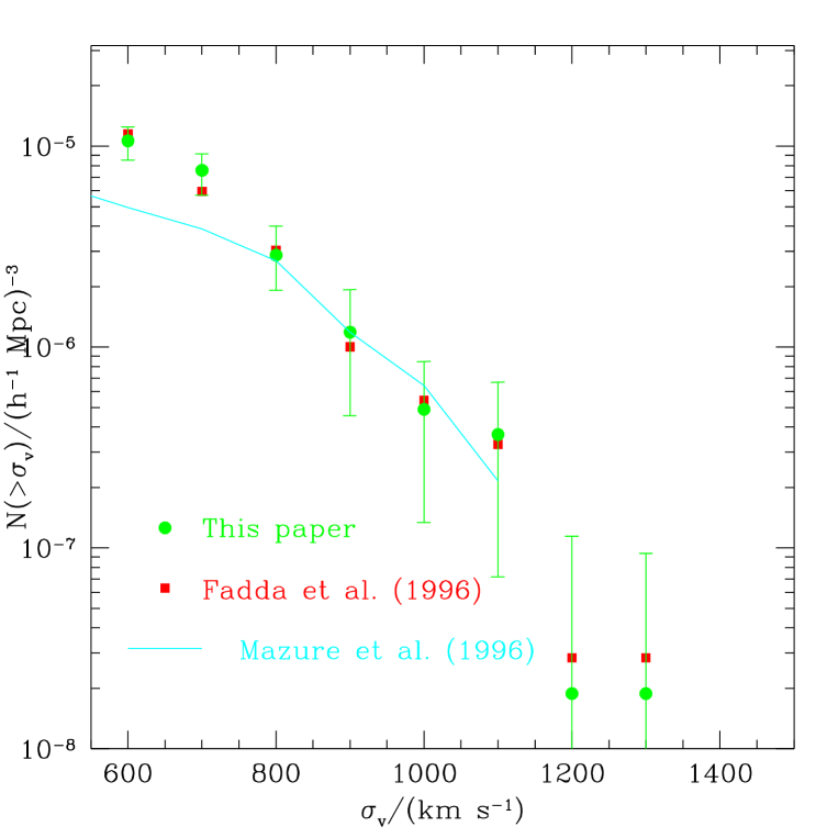
Figure 1: The cumulative velocity dispersion function for the observational sample as originally published by F96 (squares) and re-estimated here (circles). The continuous line represents the determination by Mazure et al. (1996) for ENACS clusters. Errorbars are the 1$\sigma$ uncertainties obtained by adding in quadrature errors coming from the Poissonian statistics and from the bootstrap error in the determination of individual cluster velocity dispersions.

We compare in Figure 1 the original $N(>\sigma_{v})$ from F96 (squares) to the one we calculated here (circles). Also plotted is the CVDF obtained by M96 for the ENACS clusters (continuous line). As already pointed out in the Introduction, the ENACS sample is incomplete for $\sigma_{v}\raise-2.0pt\hbox{\hbox to0.0pt{\hbox{$\sim$}\hss}\raise 5.0pt\hbox{$<$}\ }800\,{\rm km\,s^{-1}}$. This explains the bending of its $N(>\sigma_{v})$ in this velocity range. As for the F96 sample, it is remarkable the agreement with the original $N(>\sigma_{v})$ estimate. This indicates that, at least from a statistical point of view, velocity gradients and galaxy morphology play a marginal role. In turn, these results are very close to those by M96 in the range of completeness of the ENACS. The plotted errorbars (reported only in one case for sake of clarity) represent the $1\sigma$ uncertainties obtained by summing in quadrature the Poissonian errors and the bootstrap errors in the determination of $\sigma_{v}$ for each individual cluster. Note that Poissonian errors are due to the fact that we sample the intrinsic $N(>\sigma_{v})$ distribution with a finite number of clusters, while bootstrap errors are connected to the finite sampling of the velocity dispersion within individual clusters. Therefore, such errors have independent origin and must both be considered.

In the following, our CVDF will be used for the comparison with simulation results.

4.2 Testing the method

We will test here the reliability of the method for cluster membership assignment, that we described in the previous section. We will also compare the resulting $\sigma_{v}$ estimates to the intrinsic ones, as provided by using the whole 3D information from the simulation particle distribution. After analysing how projection and sampling biases affect the determination of the velocity dispersion, we will also show their overall imprint on $N(>\sigma_{v})$.

We plot in Figure 2 the result of introducing observational biases on four clusters selected from the TCDM model with $\sigma_{8}=0.67$. The first three clusters from the left have progressively larger $\sigma_{v}$ values, while the fourth column shows the case of a cluster which is rejected on the ground of its too large $\sigma_{v}$ bootstrap error [$>150\,{\rm km\,s^{-1}}$; cf. point (3) in the previous section]. Panels in the first line show how the clusters appear in projection, with open circles indicating the rejected interlopers and filled circles for the “galaxies” recognized as genuine members. We note that the algorithm for membership assignment is rather efficient in identifying interlopers preferentially at the outskirts of the clusters, while genuine members are more concentrated to define the cluster shape. This is also confirmed by the panels in the second line, which show the real–space distribution along the line of sight for accepted (filled histogram) and rejected (open histogram) members. In general, true members of the first three clusters are correctly recognized to lie very close to the cluster center, with few exceptions (e.g., note the group of seven galaxies, located at $\simeq 20\,h^{-1}{\rm Mpc}$ from the center of the second cluster). As for the fourth cluster, a non–negligible fraction of galaxies recognized as genuine members are instead interlopers, which lie at a distance $\raise-2.0pt\hbox{\hbox to0.0pt{\hbox{$\sim$}\hss}\raise 5.0pt\hbox{$>$}\ }20\,h^{-1}{\rm Mpc}$ from the cluster.

Figure 2: Results of the application of the cluster member assignment and $\sigma_{v}$ estimate on four clusters extracted from the TCDM simulations with $\sigma_{8}=0.67$. Panels in the first line show clusters in projection. Filled and open circles refer to “galaxies” recognized as genuine members and interlopers, respectively. Panels in the second and third lines show the histograms for the line–of–sight galaxy distribution toward the cluster centers in real and velocity space, respectively. Open and filled histograms are for the distributions of interlopers and true cluster members. Panels in the fourth line are for the integral velocity dispersion profiles. The horizontal dashed line corresponds to the intrinsic $\sigma_{v}$ value, computed at $1.5\,h^{-1}{\rm Mpc}$. Errorbars are for the r.m.s. scatter over 1000 bootstrap resamplings. For each cluster the point at the smallest radius represents $\sigma_{v}$ as computed for the first six innermost galaxies.

Panels in the third line show the redshift–space distribution from which $\sigma_{v}$ is actually calculated, while the fourth line shows the projected integrated velocity dispersion profile. In each panel the horizontal dashed line represents the intrinsic value of $\sigma_{v}$, which is estimated from all the simulation particles lying within $1.5\,h^{-1}{\rm Mpc}$ from the cluster center. Errorbars are the $1\sigma$ scatter from 1000 bootstrap resamplings. As for the first two clusters, it is remarkable how well the correct $\sigma_{v}$ is recovered at the scales where it keeps flat (see F96 and G96 for discussions about the flatness of profiles in the external cluster region). As for the third cluster, despite the fact that the $\sigma_{v}$ profile flattens at scales $\raise-2.0pt\hbox{\hbox to0.0pt{\hbox{$\sim$}\hss}\raise 5.0pt\hbox{$>$}\ }1\,h^{-1}{\rm Mpc}$, it does not converge to the correct value. Note that the discrepancy of $\sim 200\,{\rm km\,s^{-1}}$ exists at a high confidence level ($>3\sigma$) and, therefore, can not be ascribed to sampling uncertainties. This means that a better recovering of the intrinsic $\sigma_{v}$ can hardly be attained in this case with a denser galaxy sampling. The situation is quite different for the fourth cluster. In this case, the discrepancy is as large as $\sim 400\,{\rm km\,s^{-1}}$, but it is not significant, as a consequence of the large errorbars. This example shows the effectiveness of eliminating those clusters with large $\sigma_{v}$ errors, which in general corresponds to rather small and loose structures, whose $\sigma_{v}$ can be heavely boosted by sampling uncertainties.

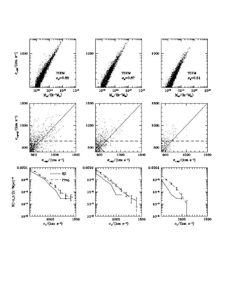
Figure 3: Effect of the observational biases on the $\sigma_{v}$ estimates for the three TCDM outputs. Panels in the first line show the relation between intrinsic velocity dispersion and cluster masses, both estimated at $1.5\,h^{-1}{\rm Mpc}$. Panels in the second line show the scatter between intrinsic and observed cluster velocity dispersions. The horizontal dashed line is for the $\sigma_{v}$ completeness limit of the F96 sample, $\sigma_{v,lim}=650\,{\rm km\,s^{-1}}$. Panels in the third line are for the intrinsic (solid lines) and observational (dashed lines) CVDF. Errorbars represent the 1$\sigma$ Poissonian uncertainty.

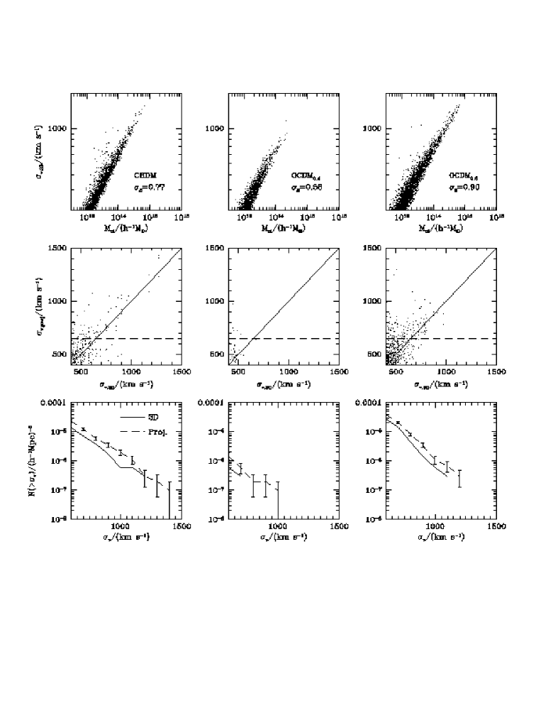
Figure 5: The same as in Figure 3, but for CHDM, OCDM_0.4 and OCDM_0.6 simulations.

Figures 3–5 are devoted to the statistical description of what can be understood from measurements of cluster internal velocity dispersion. Results are reported for all the nine simulation outputs that have been considered (for each model, plotted results refer to only one realization). The panels in the first line show the relation between the intrinsic $\sigma_{v,3D}$, estimated by using all the simulation particles within $1.5\,h^{-1}{\rm Mpc}$, and the total cluster mass within the same radius (as for CHDM, both quantities refer only to the cold particles). We note that a well defined correlation always exists, which reflects the condition of virial equilibrium characterizing most of the clusters. Few clusters detach significantly from this correlation and all have velocity dispersions larger than the virialization one. Such exceptions are even more rare for those models, like the OCDM ones, in which the cluster particles have spent more time within the collapsed structure and, therefore, have had more time to reach virial equilibrium.

Note that a scatter of a factor two in mass at a fixed $\sigma_{v}$ value is not rare, especially at low $\sigma_{v}$ values. However, one would conclude that in general rather reliable cluster mass determinations would be possible from measurements of the internal velocity dispersion. The situation is rather different in realistic cases, when observational limitations are introduced. This is shown in the panels of the second line, where we plot the relation between the projected $\sigma_{v}$, estimated according to the procedure described in Section 3, and the intrinsic $\sigma_{v}$. Although most of the clusters show discrepancies of about 100–200$\,{\rm km\,s^{-1}}$ between observed and true velocity dispersions, there are cases in which the difference is as large as $\sim 500\,{\rm km\,s^{-1}}$.

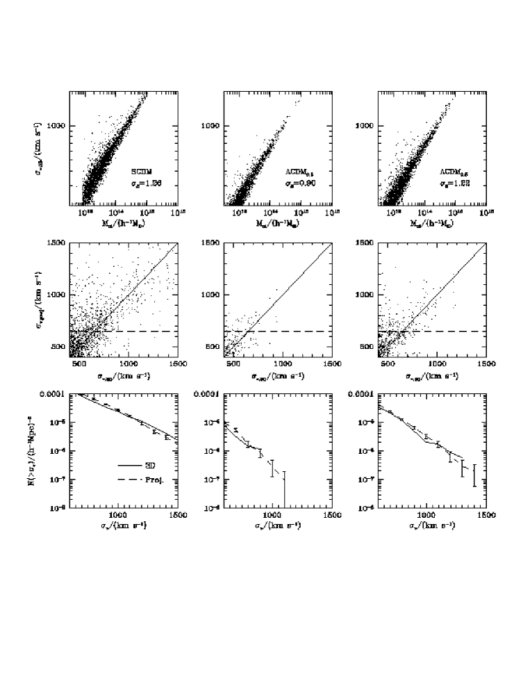
Figure 4: The same as in Figure 3, but for SCDM, $\Lambda$CDM_0.3 and $\Lambda$CDM_0.5 simulations.

The consequence of the large scatter in the $\sigma_{v,proj}$–$\sigma_{v,3D}$ on $N(>\sigma_{v})$ is plotted in the panels of the third line, where we compare the CVDF for the intrinsic (solid lines) and observed (dashed lines) velocity dispersions. Errorbars, which are reported only for the “observational” CVDF, represent the Poissonian uncertainties. As expected, the overall effect is that of increasing the CVDF, especially in the large $\sigma_{v}$ tail. This result is qualitatively similar to that found by van Haarlem et al. (1997). A closer comparison with his analysis is however rather difficult, since he considered simulations only of the SCDM model with $\sigma_{8}=0.63$, by adopting a lower mass resolution, although within a larger simulation box. Furthermore, he also used different procedures to remove observational biases in the $\sigma_{v}$ estimate.

We point out that all the results we reported here are based on clusters whose $3D$ velocity dispersion is larger than $\sigma_{lim,3D}=400\,{\rm km\,s^{-1}}$. Since we require that simulated cluster samples be complete above $\sigma_{lim,proj}=650\,{\rm km\,s^{-1}}$ (indicated with the horizontal dashed line), we should keep $\sigma_{lim,3D}$ small enough that no clusters below this limit would have their $\sigma_{v,proj}$ increased above the observational completeness limit. On the other hand, the number of selected clusters rapidly increases as $\sigma_{lim,3D}$ decreases, so as to hardly keep the amount of data to be analysed to a manageable size. We verified that the incompleteness induced in the simulated samples by taking $\sigma_{lim,3D}=400\,{\rm km\,s^{-1}}$ is always negligible (note that only very few clusters have $\sigma_{v,proj}>650\,{\rm km\,s^{-1}}$ at the smallest $\sigma_{v,3D}$). Indeed, for the TCDM model with $\sigma_{8}=0.67$ we plot the observed $N(>\sigma_{v})$ obtained from $\sigma_{lim,3D}=400\,{\rm km\,s^{-1}}$ (short–dashed curve) and $\sigma_{lim,3D}=200\,{\rm km\,s^{-1}}$ (long–dashed curve). The small difference between these two cases confirms the reliability of cutting at $\sigma_{lim,3D}=400\,{\rm km\,s^{-1}}$.

Note that the difference with respect to the intrinsic $N(>\sigma_{v})$ is rather model dependent being in general smaller for those models whose clusters have had more time to virialize; an excellent recovering of the 3D cumulative distribution is indeed found for SCDM and $\Lambda$CDM_0.5, which have the largest $\sigma_{8}$ values; instead, larger differences exist for TCDM as lower $\sigma_{8}$ values are considered. Also note how models whose intrinsic $N(>\sigma_{v})$ are comparable, like $\Lambda$CDM_0.3 and TCDM with $\sigma_{8}=0.51$ are affected in a rather different way by observational biases. The CVDF for $\Lambda$CDM_0.3 is almost unaffected at $\sigma_{v}\raise-2.0pt\hbox{\hbox to0.0pt{\hbox{$\sim$}\hss}\raise 5.0pt\hbox{$<$}\ }900\,{\rm km\,s^{-1}}$, while it only acquires a high $\sigma_{v}$ tail up to $\sigma_{v}\simeq 1100\,{\rm km\,s^{-1}}$. On the other hand, the low–$\sigma_{8}$ TCDM significantly increases its CVDF over the whole $\sigma_{v}$ range. This is due to the fact that $\Lambda$CDM_0.3 clusters are small and rather isolated structures, which already undergone virialization. As a consequence, the effect of interlopers is in general smaller than for TCDM clusters, which are expected to be more extended objects (like in any $\Omega_{0}=1$ model) characterized by the presence of substructures and continuous merging of surrounding clumps. This is explicitely shown in Figure 6, where we plot the structure and velocity dispersion profiles for two clusters extracted from a $\Lambda$CDM_0.3 and a TCDM ($\sigma_{8}=0.51$) simulation. Left and central panels show in projection the whole particle distribution within the observational cylinder, before and after the inclusions of the observational biases, respectively. Since the two simulations are started with the same initial random numbers and the two clusters lie almost at the same position, they are originated by the same waves and any difference in their morphology is only due to the difference in the corresponding cosmologies. The cluster in $\Lambda$CDM_0.3 has a much better defined shape than that in TCDM. The latter, even after the interloper removal, does not look in projection like a well defined structure. As a consequence, the membership assignment is not very efficient in identifying genuine cluster members and the resulting velocity dispersion profile does not recover the true $\sigma_{v}$ so efficiently like for the $\Lambda$CDM_0.3 cluster.

The results of this analysis can be summarized into two main points.

(a)

Although the scatter between the intrinsic and the observed $\sigma_{v}$ is in general rather large, the difference between the corresponding $N(>\sigma_{v})$ is not dramatic, especially for $\sigma_{v}\raise-2.0pt\hbox{\hbox to0.0pt{\hbox{$\sim$}\hss}\raise 5.0pt\hbox{$<$}\ }800\,{\rm km\,s^{-1}}$. This is just the consequence of the roughly symmetric distribution of overestimates and underestimates of $\sigma_{v}$. Discrepancies in the high $\sigma_{v}$ tail are due to few clusters whose $\sigma_{v}$ ought to be overestimated by 200–300$\,{\rm km\,s^{-1}}$, because of the presence of unremoved interlopers. A typical example of this occurrence is just provided by the third cluster in Figure 2.

(b)

Differences between intrinsic and observed $N(>\sigma_{v})$ may however not be negligible. Furthermore, no a priori recipe exists, which could allow to recover the correct CVDF from the observed one, the difference being non–trivially model dependent. This casts doubts on the reliability of detailed comparisons between the abundance of clusters, as inferred from their internal velocity dispersion, and predictions of DM models based on analytical approaches, like the Press & Schechter (1974) one, which can not include any observational effect.

4.3 Comparing with DM models

Based on the results obtained in the previous sections, we compare in Figure 7 the CVDF for the observational sample and for the simulations. In each panel, the shaded band represents the result of our analysis of the F96 sample (cf. Figure 1 and Section 4.1). For each model, results are obtained by averaging over the three available realizations (exept for CHDM).

As for the SCDM model, as expected it largely overproduces clusters at any $\sigma_{v}$. In order to check for the effect of a possible velocity bias on this model, we resorted to the relation $b_{v}=0.7(r/0.5\,h^{-1}{\rm Mpc})^{0.2}$ ($b_{v}$: ratio between the velocity dispersions of “galaxies” and dark matter particles) obtained by Evrard et al. (1994) from hydrodynamical cluster simulations of a CDM model with $\sigma_{8}=0.6$. Since these authors found the above relation to be almost independent of the evolutionary stage, we adopt it also for our larger $\sigma_{8}$ output (cf. Table 1). The effect of such a velocity bias is shown with the dotted curve in the upper left panel; even in this case the resulting $N(>\sigma_{v})$ is much larger than the observational one.

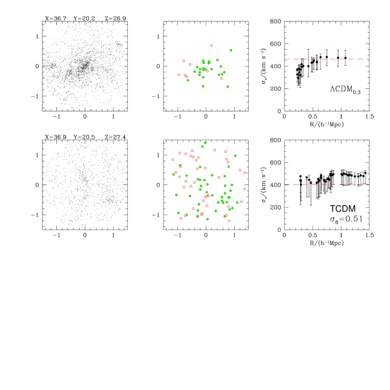
Figure 6: Comparison of the role of projection effects on a cluster identified in $\Lambda$CDM_0.3 (upper panels) and TCDM with $\sigma_{8}=0.51$ (lower panels) simulations. Note that the two clusters have almost the same positions in the two simulations based on the same set of initial random numbers. Left panels show in projection the whole distribution of simulation particles within the observational cylinder. Central and right panels are the same as for plots in the first and fourth lines of Fig. 2.

From the results reported in lower left panel, it turns out that lowering the primordial spectral index to $n=0.85$ is not enough to bring a $\Omega_{0}=1$ CDM model into agreement with observations, unless one introduces a substantial amount of gravitational wave contribution to the CMB anisotropy. Even taking $T/S=7(1-n)$ from power–law inflation ($\sigma_{8}=0.67$), the CVDF remains significantly larger than that of the observational sample. Only further lowering the normalization to $\sigma_{8}=0.51$ leads into agreement with real data, thus in accordance with the X–ray based results (see, e.g., E96; Pen 1996). In their analysis of the large–scale velocity fields, Zaroubi et al. (1997) found that TCDM with $n\simeq 0.85$ is the best fit for $\Omega_{0}=1$, $h=0.5$ CDM models only if $T/S=0$ (see, however, Borgani et al. 1997b). A possible way out may be allowing for a substantially larger baryon fraction (see, e.g., White et al. 1996). This would have the effect of suppressing fluctuations on the cluster mass scale, while leaving the spectrum almost unchanged at the larger scales probed by velocity fields.

As for the CHDM model, it turns out to marginally overproduce clusters. A better agreements can be achieved either by increasing the hot component or by tilting the primordial spectral index. In both cases this model, which is already marginally consistent with observations of high–redshift ($z=3$–4) damped Ly$\alpha$ systems, would have even harder time with the galaxy formation timing (see, e.g., Borgani et al. 1996, and references therein). A way to overcome this problem would be to share the hot component between more than one $\nu$ species; in this case, the increase in the neutrino free streaming suppress fluctuations on the cluster mass scale, without significantly affecting the fluctuation power on the galaxy mass scale. A model with $\Omega_{\nu}=0.2$ and two massive neutrinos (Primack et al. 1995; Primack 1996) has been found to satisy at the same time the constraints from the cluster abundance and high–redshift objects.

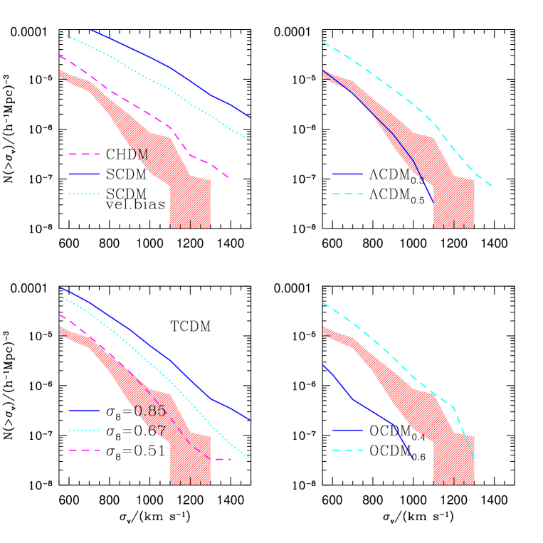
Figure 7: Comparisons between CVDF’s for real data (dashed band) and simulations. Simulation results correspond to the average over the three random realization of each model (except for CHDM, for which only one realization is available).

In any case, it is interesting to note that the CHDM model, for which $\sigma_{8}=0.77$, has a CVDF which is comparable to (or even smaller than) that of TCDM with $\sigma_{8}=0.67$, even though $\Omega_{0}=1$ for both models. This is the consequence of the presence of the neutrino component, which acts like a sort of background superimposed on the more clustered cold component. Its effect is that of slowing down the dynamical clustering evolution, so that more time is required for a CHDM model to develop the same small–scale velocities of a purely cold model. This means that a larger $\sigma_{8}$ value is required for a CHDM model to produce the same cluster abundance as an $\Omega_{0}=1$ CDM model.

As for the $\Lambda$CDM models, the $\Omega_{0}=0.3$ case is quite consistent with the observational $N(>\sigma_{v})$, thus confirming the result based on $X$–ray data about the capability of this model to produce the correct cluster abundance (see, e.g., E96). The $\Lambda$CDM_0.5 model, instead, turns out to overproduce clusters, as expected on the ground of its large $\sigma_{8}$ value. As for OCDM, the $\Omega_{0}=0.4$ model is found to underproduce clusters, while increasing the density parameter to $\Omega_{0}=0.6$ turns into a marginal cluster overproduction.

5 Conclusions

In this paper we addressed the question concerning the reliability of the distribution of cluster internal velocity dispersions as a diagnostic for cosmological models. In order to properly address this issue we decided: (a) to run simulations for a variety of models, so as to verity the discriminative power of $N(>\sigma_{v})$; (b) to analyse simulated clusters in the same way as a reference observational sample, originally considered by Fadda et al. (1996; F96), consisting of 153 clusters and complete in velocity dispersion down to $\sigma_{v,lim}\simeq 650\,{\rm km\,s^{-1}}$.

Our main results can be summarized as follows.

(a)

Projection effects and the limited number of galaxy redshifts per cluster can heavily pollute the recovering of the correct $\sigma_{v}$. The cluster member selection procedure leads to the wrong identification of several interlopers as genuine members. This effect is more pronounced for low–$\sigma_{v}$ ($\raise-2.0pt\hbox{\hbox to0.0pt{\hbox{$\sim$}\hss}\raise 5.0pt\hbox{$<$}\ }600\,{\rm km\,s^{-1}}$) objects. On the other hand, high–$\sigma_{v}$ clusters, which look in projection like better defined structures, display an improved recovering of the true $\sigma_{v}$.

(b)

The resulting effect is in general that of overestimating the CVDF, especially in the high–$\sigma_{v}$ tail. This is due to few small, low–$\sigma_{v}$ clusters, whose velocity dispersion is heavily boosted by projection effects. Furthermore, the amount of the overestimate is non–trivially model dependent: simulations in which particles last more within virialized structures generate clusters with a sharper profile, even after projection, so as to make interloper removal an easier task.

(c)

As for the comparison with data, our results substantially agree with the $\sigma_{8}$–$\Omega_{0}$ scaling for CDM models, based on the Press–Schechter approach to the $X$–ray temperature function (e.g., Viana & Liddle 1996; Eke et al. 1996; Pen 1996). We confirm that a $\Omega_{0}=1$ CDM model requires $\sigma_{8}\simeq 0.5$. The $\Lambda$CDM model with $\Omega_{0}=0.3$ produces the correct $N(>\sigma_{v})$ with $\sigma_{8}=1.1$. This value is somewhat larger than that predicted by Eke et al. (1996; cf. Table 1), but rather consistent with the scaling provided by Pen (1996). As for the CHDM model, it overproduces clusters, although not by a large amount. In any case, the presence of the neutrino background has the effects of slowing down the development of non–linear structures. As a consequence, CHDM models are allowed to have a larger $\sigma_{8}$ value to provide the same cluster abundance as an $\Omega_{0}=1$ CDM model (see also Jing & Fang 1994 and Walter & Klypin 1996). This is the reason why the CVDF for CHDM with $\sigma_{8}=0.77$ is smaller than that of TCDM with $\sigma_{8}=0.67$.

Such constraints on $\sigma_{8}$ from cluster abundance can be compared with those from large–scale velocity fields. For instance, Zaroubi et al. (1997) found for CDM models that $\sigma_{8}\Omega_{0}^{0.6}=0.88\pm 0.15$ ($90\%$ c.l.) is predicted by a maximum likelyhood approach to the peculiar velocities of the Mark III sample. Instead, Borgani et al. (1997b) analysed the sample of cluster peculiar velocities by Giovanelli et al. (1997) and derived $\sigma_{8}\Omega_{0}^{0.6}=0.5\pm 0.2$ ($90\%$ c.l.), thus in better agreement with cluser abundance.

Based on such results, we conclude that cluster internal velocity dispersions represent a stringent cosmological constraint, provided that observational biases, like projection and sampling effects, are carefully accounted for (cf. also van Haarlem et al. 1997). It is also clear that further advancements both from the theoretical and the observational sides would be required in order to fully exploit the potential of cluster velocity dispersions. For instance, the availability of high–resolution simulations, also including gas dynamics, should settle the question of the velocity bias, whose amount should be rather model dependent.

Furthermore, improved observational strategies should eliminate some of the ambiguities, which are still present in the data sets. The possibility of measuring many more galaxy redshifts per cluster will allow a better understanding of the internal cluster dynamics and of the role of substructures. Extensions of the today available samples in the following two directions would provide even more stringent constraints on DM models. From the one hand, realising a shallower volume–limited ($z\raise-2.0pt\hbox{\hbox to0.0pt{\hbox{$\sim$}\hss}\raise 5.0pt\hbox{$<$}\ }0.1$) survey, including at least down to $R=0$ clusters, would extend to smaller $\sigma_{v}$ the range where the CVDF is accurately sampled. From the other hand, realising a deeper ($z\raise-2.0pt\hbox{\hbox to0.0pt{\hbox{$\sim$}\hss}\raise 5.0pt\hbox{$>$}\ }0.5$) survey of rich clusters would allow to discriminate between those models that, even though providing the correct $N(>\sigma_{v})$ at $z\simeq 0$, have different evolutionaly patterns (e.g., Jing & Fang 1993; Crone & Geller 1994). Attempts in this direction have been already pursued with the CNOCC cluster survey (see, e.g., Carlberg et al. 1996, and references therein), but only for a limited number of clusters. In any case, it is clear that as deeper cluster surveys are considered, a careful treatment of projection biases becomes a more and more delicate issue. Multi–object spectrographs of the new generation will be needed to measure $\sim 10^{2}$ galaxy redshifts for each cluster in one shot, thus rendering feasible in the near future a substantial enlargment of the today available data sets.

References

Abell G.O., Corwin H.G., Olowin R.P., 1989, ApJS, 70, 1
Bahcall N.A., Cen R., 1993, ApJ, 407, L49
Balland C., Blanchard A., 1996, preprint
Bardeen J.M., Bond J.R., Kaiser N., Szalay A.S., 1986, ApJ, 304, 15
Bartelmann M., 1995, A&A, 303, 643
Bartlett J.G., Silk J., 1993, ApJ, 407, L45
Beers T.C., Flynn K., Gebhardt K., 1990, AJ, 100, 32
Bennett C.S., et al., 1996, ApJ, 464, L1
Bird C.M., 1995, ApJ, 445, L81
Bird C.M., Mushotzki R.F., Metzler C.A., 1996, ApJ, 1995, 453, 40
Biviano A., Girardi M., Giuricin G., Mardirossian F., Mezzetti M., 1993, ApJ, 411, L13
Bond J.R., Jaffe A.H., 1996, Proceedings of the XXXI Moriond meeting “Microwave Background Anisotropies”, preprint astro–ph/9610091
Borgani S., da Costa L.N., Freudling W., Giovanelli R., Haynes M., Salzer J., Wegner G., 1997, ApJ Letters, submitted
Borgani S., Lucchin F., Matarrese S., Moscardini L., 1996, MNRAS, 280, 749
Borgani S., Moscardini L., Plionis M., Górski K.M., Holtzman J., Klypin A., Primack J.R., Smith C.C., Stompor R., 1997a, NewA, 1, 321
Bunn E.F., Liddle A.W., White M., 1996, Phys. Rev., D54, 5917
Buote D.A., Tsai J.C., 1996, ApJ, 458, 27
Burles S., Tytler D., 1996, Science, submitted, preprint astro–ph/9603070
Carlberg R.G., 1994, ApJ, 433, 468
Carlberg R.G., Morris S.L., Yee H.K.C., Ellingson E., 1996, ApJ Letters, in press, preprint astro–ph/9612169
Cen R., 1996, preprint astro–ph/9608070
Collins C.A., Guzzo L., Nichol R.C., Lumsden S.L., 1995, MNRAS, 274, 1071
Copi C.J., Schramm D.N., Turner M.S., 1995, Phys. Rev. Lett., 75, 3981
Couchman H.M.P., 1991, ApJ, 268, L23
Crittenden R., Bond J.R., Davis R.L., Efstathiou G., Steinhardt P.J., 1993, Phys. Rev. Lett., 71, 324
Crone M.M., Evrard A.E., Richstone D.O., 1996, ApJ, 467, 489
Crone M.M., Geller M.J., 1994, AJ, 110, 21
David L.P., Jones C., Forman W., 1995, ApJ, 445, 578
Dell’Antonio I.P., Geller M.J., Fabricant D.G., 1994, AJ, 107, 427
Dressler A., Schechtman S.A., 1988, AJ, 95, 985
Edge A.C., Stewart G.C., 1991, MNRAS, 252, 428
Eke V.R., Cole S., Frenk C.S., 1996, MNRAS, 282, 263 (E96)
Ensslin Q.A., Biermann P.L., Kronberg P.P., Wu X.P., 1996, ApJ, in press, preprint astro–ph/9609190
Escalera E., Biviano A., Girardi M., Giuricin G., Mardirossian F., Mezzetti M., 1994, ApJ, 423, 539
Evrard A.E., Metzler C.A, Navarro J.F., 1996, ApJ, 469, 494
Evrard A.E., Summers F.J., Davis M., ApJ, 1994, 422, 11
Fadda D., Girardi M., Giuricin G., Mardirossian F., Mezzetti M., 1996, ApJ, 473, 670 (F96)
Fields B.D., Kainulainen K., Olive K.A., Thomas D., 1996, New Ast., 1, 77
Frenk C.S., Evrard A.E., White S.D.M., Summers F.J., 1996, ApJ, 472, 460
Frenk C.S., White S.D.M., Efstathiou G., Davis M., 1990, ApJ, 351, 10
Giovanelli R., Haynes M.P., Herter T., Vogt N.P., da Costa L.N., Freudling W., Wegner G., Salzer J.J., 1997, AJ, 113, 53
Girardi M., Biviano A., Giuricin G., Mardirossian F., Mezzetti M., 1993, ApJ, 404, 38
Girardi M., Fadda D., Giuricin G., Mardirossian F., Mezzetti M., Biviano A., 1996, ApJ, 404, 38 (G96)
van Haarlem M.P., Frenk C.S., White S.D.M., 1997, MNRAS, in press, preprint astro–ph/9701103
Henry J.P., Arnaud K.A., 1991, ApJ, 372, 410
Henry J. P., Briel U.G., 1995, ApJ, 443, L9
Jing Y.P., Fang L.Z., 1994, ApJ, 432, 438
Katgert P., Mazure A., Perea J., et al., 1996, A&A, 310, 8
Katz N., Hernquist L., Weinberg D.H., 1992, ApJ, L109
Klypin A., Nolthenius R., Primack J.R., 1996, ApJ, in press, preprint astro–ph/9502062
Kochanek C.S., 1995, ApJ, 453, 545
Lacey C., Cole S., 1994, MNRAS, 271, 676
Lineweaver C.H., Barbosa D., Blanchard A. Bartlett J.G., 1996, A&A, submitted, preprint astro–ph/9610133
Loeb A., Mao S., 1994, ApJ, 435, L109
Lubin L.M., Bahcall N.A., 1993, ApJ, 415, L17
Lubin L.M., Cen R., Bahcall N.A., Ostriker J.P., 1996, 460, 10
Lumsden S.L., Nichol R.C., Collins C.A., Guzzo L., 1992, MNRAS, 258, 1
Ma C.P., 1996, ApJ, 471, 000, preprint astro–ph/9605198
Mazure A., Katgert P., den Hartog R., et al., 1996, A&A, 310, 31
Merritt D., 1987, ApJ, 313, 121
Miralda–Escudè J., Babul A., 1995, ApJ, 449, 18
Mohr J.J., Evrard A.E., Fabricant D.G., Geller M.J., 1995, ApJ, 447, 8
Navarro J.F., Frenk C.S., White S.D.M., 1995, MNRAS, 275, 720
Oukbir J., Blanchard A., 1996, A&A, submitted, preprint astro–ph/9611085
Pen U.L., 1996, ApJ, submitted, preprint astro–ph/9610147
Pen U.L., Spergel D.N., Turok N., 1994, Phys Rev., D49, 692
Pisani A., 1993, MNRAS, 265, 706
Pisani A., 1996, MNRAS, 278, 697
Press W.H., Schechter P., 1974, ApJ, 187, 425
Primack J.R., Holtzman J., Klypin A., Caldwell D.O., 1995, Phys. Rev. Lett., 74, 2160
Primack, J. R. 1996, in Critical Dialogues in Cosmology, ed. Neil Turok (World Scientific, in press), astro-ph/9610078
Reeves H., 1994, Rev. Mod. Phys., 66, 193
Seitz S., Schneider P., 1996, A&A, 305, 383
Squires G., Kaiser N., 1996, ApJ, 469, 73
Stein P., 1996, A&A, in press, preprint astro–ph/9606162
Sugiyama N., 1995, ApJS, 100, 281
Viana P.T.P., Liddle A.R., 1996, MNRAS, 281, 323
Walter C., Klypin A., 1996, ApJ, 462, 13
White M., Viana P.T.P., Liddle A.W., Scott D., 1996, MNRAS, 283, 107
White M., Scott D., 1996, Comm. Ap., 18, 289
White S.D.M., Efstathiou G., Frenk C.S., 1993a, MNRAS, 262, 1023
Wu X.P., Fang L.Z., 1997, ApJ, in press, preprint astro–ph/9701196
Zabludoff A.I., Huchra J.P., Geller M.J., 1990, ApJS, 74, 1
Zabludoff A.I., Geller M.J., Huchra J.P., Ramella M., 1993, AJ, 106, 1301
Zaroubi S., Dekel A., Hoffman Y., Kolatt T., 1997, ApJ, in press, preprint astro-ph/9610226