Dynamical stability of N-body models for M32
with a central black hole

Abstract

We study the stability of stellar dynamical equilibrium models for M32. Kinematic observations show that M32 has a central dark mass of $\sim 3\times 10^{6}\>{\rm M_{\odot}}$, most likely a black hole, and a phase-space distribution function that is close to the ‘two-integral’ form $f=f(E,L_{z})$. M32 is also rapidly rotating; 85–90% of the stars have the same sense of rotation around the symmetry axis. Previous work has shown that flattened, rapidly rotating two-integral models can be bar-unstable. We have performed N-body simulations to test whether this is the case for M32. This is the first stability analysis of two-integral models that have both a central density cusp and a nuclear black hole.

Particle realizations with $N=\>$512,000 were generated from distribution functions that fit the photometric and kinematic data of M32. We constructed equal-mass particle realizations, and also realizations with a mass spectrum to improve the central resolution. Models were studied for two representative inclinations, $i=90^{\circ}$ (edge-on) and $i=55^{\circ}$, corresponding to intrinsic axial ratios of $q=0.73$ and $q=0.55$, respectively. The time evolution of the models was calculated with a ‘self-consistent field’ code on a Cray T3D parallel supercomputer. We find both models to be dynamically stable. This implies that they provide a physically meaningful description of M32, and that the inclination of M32 (and hence its intrinsic flattening) cannot be strongly constrained through stability arguments.

Previous work on the stability of $f(E,L_{z})$ models has shown that the bar-mode is the only possibly unstable mode for systems rounder than $q\approx 0.3$ (i.e., E7), and that the likelihood for this mode to be unstable increases with flattening and rotation rate. The $f(E,L_{z})$ models studied for M32 are stable, and M32 has a higher rotation rate than nearly all other elliptical galaxies. This suggests that $f(E,L_{z})$ models constructed to fit data for real elliptical galaxies will generally be stable, at least for systems rounder than $q\gtrsim 0.55$, and possibly for flatter systems as well.

1 Introduction

Active galaxies and quasars are thought to be powered by the presence of massive black holes (BHs) in their nuclei (e.g., Rees 1997). Such BHs are believed to exist in a large fraction of quiescent galaxies as well (e.g., Tremaine 1996). The best dynamical BH detections in active galaxies come from studies of gas kinematics; in quiescent galaxies only stars are generally available as a tracer of the gravitational potential. Ground-based stellar kinematical studies have yielded tentative detections for BHs in a handful of nearby quiescent galaxies (Kormendy & Richstone 1995), and this evidence is now being improved with the superior spatial resolution of the Hubble Space Telescope (HST; Kormendy et al. 1996a,b; van der Marel et al. 1997a). However, the interpretation of the observed stellar motions is never straightforward; only projected quantities are observed and the three-dimensional orbital structure is unknown. Construction of detailed dynamical models is therefore required. Axisymmetric models currently provide the state-of-the-art for this application. In such models, the phase-space distribution function (DF) generally depends on three integrals of motion (e.g., Binney & Tremaine 1987), the two classical integrals, $E$ and $L_{z}$ (the binding energy and the angular momentum component along the symmetry axis, both per unit mass), and the third integral, $I_{3}$. The latter cannot generally be expressed analytically in terms of the phase-space coordinates, which makes the construction of models with ‘three-integral’ DFs, $f=f(E,L_{z},I_{3})$, complicated and time-consuming, although not impossible (Dehnen & Gerhard 1993; Cretton et al. 1997; Gebhardt et al. 1997). As a result, significant attention has been given in recent years to a special class of axisymmetric models, those in which the DF depends only on the two classical integrals of motion, $f=f(E,L_{z})$. The attraction of these ‘two-integral’ models lies in the fact that their properties are tractable semi-analytically (e.g., Hunter & Qian 1993; Dehnen & Gerhard 1994). These models can be viewed as the axisymmetric generalization of spherical isotropic models: the velocity dispersions in the meridional plane are isotropic, i.e., $\sigma_{r}=\sigma_{\theta}$, and the flattening of the models (when oblate) is due to an excess of azimuthal motion.

The present paper deals with the nearby E3 galaxy M32, which has been a strong candidate for containing a BH for many years. The highest spatial resolution ground-based data are well fit by an $f(E,L_{z})$ model with a 2–$3\times 10^{6}\>{\rm M_{\odot}}$ BH (van der Marel et al. 1994; Qian et al. 1995; Dehnen 1995; Bender, Kormendy & Dehnen 1996). Such a model fits the observed line-of-sight velocity profile shapes without any adjustable parameters, suggesting that the DF of M32 is indeed close to the $f(E,L_{z})$ form. We recently completed the most detailed study to date of M32 (van der Marel et al. 1997a), using new HST data (van der Marel, de Zeeuw & Rix 1997b) and fully general three-integral modeling (van der Marel et al. 1997c; hereafter vdM97c). The main results of these studies are that: (i) M32 must have a central dark mass in the range $M_{\bullet}=(3.4\pm 1.6)\times 10^{6}\>{\rm M_{\odot}}$ (at the formal $99.73$% confidence level), enclosed within $\sim 0.3\>{\rm pc}$, most likely a BH; and (ii) the best-fitting models have a dynamical structure that is indeed similar (although not identical) to that of an $f(E,L_{z})$ model.

Although dynamical models with $f(E,L_{z})$ DFs can reproduce most features of the M32 data, they must also be stable if they are to be physically meaningful. Only limited research has been done on the stability of $f(E,L_{z})$ models. Bending modes and lopsided modes in extremely flattened systems (axial ratio $q\lesssim 0.2$) were discussed by Merritt & Fridman (1995). Kuijken & Dubinski (1994) performed N-body simulations of models with a King-type mass density profile and an axial ratio varying between $q\approx 0.6$ in the center and $q\approx 0.8$ in the outer parts. Models with little or no mean streaming were stable, but rapidly rotating models were found to be unstable to the formation of a bar. Preliminary results on the bar-stability in $f(E,L_{z})$ models with central density cusps, but without central dark objects, were presented by Dehnen (1996). His N-body simulations indicate that: (i) non-rotating models are stable, even if they are as flat as $q\approx 0.3$; and (ii) maximally rotating models tend to be bar-unstable if they are flatter than $q\approx 0.5$. The most detailed study to date of the stability of $f(E,L_{z})$ models has been that for a family of Kuzmin-Kutuzov models by Sellwood & Valluri (1997). They identify all the most important unstable modes as a function of shape and rotational support. Their results confirm the main conclusions on bar modes found by earlier authors, and they also present detailed studies of lopsided, bending and other unstable modes. The introduction of their paper provides a useful reference to other recent work on the stability of hot stellar systems (see also the introductory chapter of Robijn 1995). None of the previous studies included both a central density cusp and a central black hole, as is appropriate for M32.

If M32 is being viewed edge-on, its intrinsic axial ratio is $q\approx 0.73$. The galaxy must be intrinsically flatter if it is inclined with respect to the line of sight. The observed rotation velocities imply that, over the radial range $\lesssim 20^{\prime\prime}$ for which kinematical data is available, 85–90% of the stars (more-or-less independent of the assumed inclination) must have the same sense of rotation around the symmetry axis (van der Marel et al. 1994). The previous work on the stability of $f(E,L_{z})$ models suggests that the M32 models should certainly be stable to, e.g., lopsided and bending modes (unless for extreme inclinations), but that they might be unstable to bar modes. We therefore tested the stability of the $f(E,L_{z})$ models for M32 through N-body simulations on a parallel supercomputer. Our results are described in what follows. Section 2 summarizes our choice of models, Sections 3 describes the N-body technique, and Section 4 discusses the results of the simulations. Conclusions are presented in Section 5. An appendix outlines the construction of the initial conditions.

2 Models

2.1 Distribution functions

The dynamical models that we study in this paper are based on those presented in vdM97c. The luminous mass density is assumed to be axisymmetric and of the form

$$\rho(R,z)=\rho_{0}\>(m/b)^{\alpha}\>[1+(m/b)^{2}]^{\beta}\>[1+(m/c)^{2}]^{\gamma},\qquad m^{2}\equiv R^{2}+(z/q)^{2}.$$ (1)

The intrinsic axial ratio $q$ is related to the projected axial ratio $q_{p}$ and the inclination $i$ according to $q_{p}^{2}=\cos^{2}i+q^{2}\sin^{2}i$. The parameters are set to $\alpha=-1.435$, $\beta=-0.423$, $\gamma=-1.298$, $b=0.55^{\prime\prime}$, $c=102.0^{\prime\prime}$, $q_{p}=0.73$, $\rho_{0}=j_{0}\Upsilon M_{\odot}/L_{\odot,V}$, $j_{0}=0.463\times 10^{5}(q_{p}/q)L_{\odot,V}\>{\rm pc}^{-3}$, and the distance to M32 is assumed to be $0.7\>{\rm Mpc}$. The quantity $j$ is the luminosity density, and $\Upsilon$ is the average V-band mass-to-light ratio of the stellar population. Both $\Upsilon$ and $q_{p}$ are assumed to be constant with radius. This model provides an accurate fit to the observed surface brightness profile of M32, including the available HST photometry in the central few arcsec (Lauer et al. 1992). The adopted constant $q_{p}=0.73$ provides a good approximation in the central $\sim 10^{\prime\prime}$, although at larger radii the observed ellipticity increases slowly to $0.86$ at $\sim 100^{\prime\prime}$. The model has finite mass, and two free parameters: the inclination $i$ and the mass-to-light ratio $\Upsilon$. The results of this paper do not depend on the particular parametrization (1) that is used to characterize the M32 luminosity density.

The (positive) gravitational potential of M32 is assumed to be $\Psi=\Psi_{\rm lum}+\Psi_{\rm dark}$, where $\Psi_{\rm lum}$ is the potential generated by the luminous matter with mass density (1), and $\Psi_{\rm dark}$ is the potential of a nuclear massive dark object. The latter is taken to be the ‘softened point mass’ potential

$$\Psi_{\rm dark}=GM_{\bullet}(r^{2}+\epsilon^{2})^{-1/2}.$$ (2)

This is the potential generated by a cluster with a Plummer model mass density (Binney & Tremaine 1987). For the case of a nuclear BH (i.e., a point mass) the potential is Keplerian and $\epsilon=0$. We do not include the potential of a dark halo around M32; there are no (strong) observational constraints on the possible presence and characteristics of such a dark halo. Also, if anything, adding a dark halo probably has a stabilizing effect (Ostriker & Peebles 1973; Stiavelli & Sparke 1991), and omitting a dark halo is therefore conservative in the present context.

In vdM97c, models with two- and three-integral DFs are constructed to interpret the available kinematic M32 data. Two-integral models do not reproduce all features of the data, but come close. The more general three-integral modeling shows indeed that the best-fitting models do not have two-integral DFs. However, they have a similar dynamical structure: $\overline{v_{\phi}^{2}}>\overline{v_{\theta}^{2}}\gtrsim\overline{v_{r}^{2}}$, whereas for two-integral models $\overline{v_{\phi}^{2}}>\overline{v_{\theta}^{2}}=\overline{v_{r}^{2}}$. Because the construction of $N$-body initial conditions is significantly more complicated for three-integral than for two-integral DFs, we restrict ourselves here to testing only the stability of the two-integral models for M32. We do not expect the results to be much different for more general models.

For a given gravitational potential there is a unique even DF $f_{\rm e}(E,L_{z})$ that reproduces the mass density $\rho(R,z)$. For our models we calculated this DF as described in vdM97c. The total DF is the sum of the part $f_{\rm e}$ that is even in $L_{z}$ and the part $f_{\rm o}$ that is odd in $L_{z}$. In principle $f_{\rm o}$ is determined completely by the mean streaming velocities $\overline{v_{\phi}}(R,z)$, but these are not constrained well enough by the data to make an inversion feasible. We therefore adopt a convenient parametrization for the odd part:

$$f_{\rm o}(E,L_{z})=(2\eta-1)\>f_{\rm e}(E,L_{z})\>h_{a}[L_{z}/L_{\rm max}(E)],$$ (3)

where $L_{\rm max}(E)$ is the maximum angular momentum at a given energy. The function $h_{a}$ is a smoothed step function as defined in van der Marel et al. (1994), with the parameter $a$ regulating the step-smoothness. For any given potential, the free parameters $\eta$ and $a$ can be specified so as to best fit the observed rotation velocities. Our results should not depend sensitively on the particular choice of parametrization adopted here.

2.2 Initial Conditions

We chose to simulate models with $M_{\bullet}=3\times 10^{6}\>{\rm M_{\odot}}$ and $\epsilon=0.04^{\prime\prime}$ ($=0.136\>{\rm pc}$), using $N=\>$512,000 particles. The use of a softened dark object in this context (rather than a point mass) was motivated by numerical considerations. However, the adopted value of $\epsilon$ is not inconsistent with the kinematic observations (vdM97c; the size of the smallest HST/FOS aperture is $0.086^{\prime\prime}$). There are no independent constraints on the inclination of M32, and we therefore studied models with two representative values: $i=90^{\circ}$ (edge-on) and $i=55^{\circ}$. These models have intrinsic axial ratios $q=0.73$ and $q=0.55$, respectively. For both inclinations we characterized the odd part of the DF by $\eta=1$ and $a=5.5$, which provides an adequate fit to the observed rotation velocities. The mass-to-light ratio was chosen to be $\Upsilon=2.51$ for $i=90^{\circ}$, and $\Upsilon=2.55$ for $i=55^{\circ}$. A more complete study of the influence of the assumed inclination on the stability of the models would be interesting, but also expensive in terms of computing resources.

Appendix A describes how initial conditions were generated from the DF. The most straightforward approach is to use equal-mass particles. However, even with $N=\>$512,000 equal-mass particles, the resolution near the center is poor. The solid histogram in Figure 1 shows the number of particles as function of radius $r$ for the $i=55^{\circ}$ model with equal-mass particles. To improve the resolution it is useful to adopt a spectrum of particle masses, such that particles near the center are on average less massive. This can be achieved by choosing the particle mass $\mu$ to be a decreasing function of the binding energy $E$. A convenient choice is

$$\mu(E)\propto\{\>[R_{\Psi}(E)+r_{0}]\>/\>[R_{\Psi}(E)+r_{1}]\>\}^{\lambda},$$ (4)

where $\Psi(R,z)$ is the gravitational potential, and $R_{\Psi}(E)$ is defined by $\Psi(R_{\Psi}(E),0)=E$. After some experimentation, a mass spectrum was adopted with parameters $r_{0}=0.01^{\prime\prime}$, $r_{1}=100^{\prime\prime}$ and $\lambda=1$. This yields a particle distribution that well samples the density cusp around the dark nuclear object, as well as the main body of the galaxy (Figure 1, dotted curve). For these multi-mass models (with $N=\>$512,000), particles with $r\ll r_{0}$ have $\mu\approx 5\>{\rm M_{\odot}}$, while particles with $r\gg r_{1}$ have $\mu\approx 5\times 10^{4}\>{\rm M_{\odot}}$. Figure 2 shows a scatter plot of the particle mass $\mu$ as a function of radius for the $i=55^{\circ}$ multi-mass model.

3 N-body method

We performed N-body simulations on the Cray T3D parallel supercomputer at the Pittsburgh Supercomputing Center. The ‘self-consistent field’ (SCF) code developed by Hernquist & Ostriker (1992) was used, implemented for parallel architectures as described in Hernquist, Sigurdsson & Bryan (1995) and Sigurdsson et al. (1997).

To improve the accuracy of the particle integration near the black hole, and to allow the smoothing length for the black hole to be small, the previously used standard time centered leap-frog integrator was replaced by a fourth order Hermite integration scheme (Makino 1991; Makino & Aarseth 1992). While the leapfrog has the virtue of being both simple and symplectic, a fixed time step leapfrog is vulnerable to spurious numerical scattering of orbits when potential gradients are large, e.g., in steep density cusps and deep in Keplerian potentials. Choosing a small enough fixed time step for the leapfrog integrator to be completely free of numerical scattering in the center is highly inefficient. A Hermite scheme provides a higher order, but relatively cheap integration scheme which excels at adapting to rapidly changing force terms. Since the Hermite scheme is not symplectic, global energy conservation is limited by the Poisson noise in the global potential due to the discrete realization of the potential field (see Sigurdsson & Mihos 1997 for a discussion).

A variable time step scheme was used, where the minimum time step was set by the minimum time step for any particle, using Aarseth’s condition on the force derivatives (Aarseth 1985; Makino & Aarseth 1992). To improve accuracy near the center (where time scales are short), while not slowing down the entire calculation too much, a modified two level ‘multistep’ approach was used (Sigurdsson & Mihos 1997) in which the accelerations due to the central massive object and the self-gravity of the innermost group of particles are updated more often than for the bulk of the particles at large radii. This approach speeds up the calculations by an order of magnitude relative to a single step integration. Compared to the multistep approach that we used previously (Hernquist, Sigurdsson & Bryan 1995) this approach is about twice as fast at fixed integration precision. The adaptive time step scheme is essential when the cusp is well resolved by the particle realization and the black hole smoothing length is small, to follow the particles near the center where forces and jerks are large.

The expansion uses a Hernquist (1990) model as its lowest order term, for which $\rho\propto r^{-1}$ at small radii. For the case of M32 the scale-length of this model was chosen to be $a=8.73^{\prime\prime}$. This minimizes the contribution to the potential from the higher-order terms in the expansion. The calculations are done with units in which $G=M=a=1$. In these dimensionless units, the smoothing length is $\epsilon=4.6\times 10^{-3}$, and the central dark mass is $M_{\bullet}=7.2\times 10^{-3}$. In this system of units, time is measured in units of $1.2\times 10^{6}$ yrs, and the periods of circular orbits at radii of $0.1^{\prime\prime}$, $1^{\prime\prime}$ and $10^{\prime\prime}$ are $0.095$, $1.4$ and $18$, respectively.

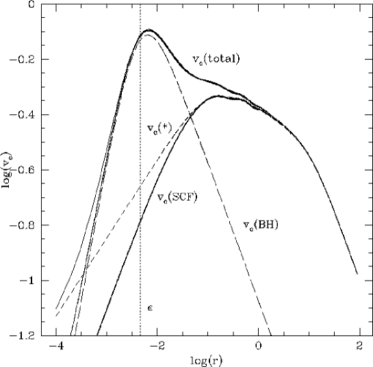
Figure 3: The circular velocity (in dimensionless units) of the $i=55^{\circ}$ model in the equatorial plane, as a function of radius (in dimensionless units). The dotted vertical line shows the softening radius $\epsilon$ of the dark object. The short-dashed curve labeled ‘$v_{\rm c}(\star)$’ is the circular velocity that corresponds to the mass density given by equation (1). The solid curve labeled ‘$v_{\rm c}({\rm SCF})$’ is the numerical approximation obtained from a SCF expansion with $n_{\rm max}=8$ terms. The approximation is poor for $\log(r)\lesssim-1.0$, due to the finite resolution of the SCF expansion. The long-dashed curve labeled ‘$v_{\rm c}({\rm BH})$’ shows the circular velocity of the (softened) black hole. The two (party overlaying) solid curves labeled ‘$v_{\rm c}({\rm total})$’ correspond to the actual total circular velocity of the model, and to the approximation obtained with the SCF expansion. The latter provides a good fit for all $\log(r)\gtrsim-2.7$, because the circular velocity at small radii is dominated by the contribution from the dark object. Hence, the numerical representation of the model is sufficiently accurate for all $r\gtrsim\epsilon$.

We performed small simulations with 25,600 and 51,200 particles to test the dependence of the results on the number of radial and angular terms in the SCF expansion. Based on these results we adopted $n_{\rm max}=8$ and $l_{\rm max}=8$ for the final simulations. Non-zero $m$ terms were included in the expansion to allow any non-axisymmetric instabilities to develop. Figure 3 illustrates the accuracy of the SCF expansion, by comparing its circular velocity to that of the true model potential. At small radii the stellar contribution to the circular velocity is poorly represented, due to the finite number of radial terms in the SCF expansion; in fact, increasing $n_{\rm max}$ by a small amount does not lead to a significantly improved fit. However, the total circular velocity is well represented for all $r\gtrsim\epsilon$, because it is dominated by the central dark object at the small radii where the SCF expansion fails. Only at radii $r\ll\epsilon$ does the numerical approximation to the total circular velocity become poor, and only as a result of the numerically imposed softening (which causes the circular velocity at $r\ll\epsilon$ to be dominated by the stellar density cusp, rather than by the dark object).

In principle, the potential could have been represented more accurately by using another set of basis functions. A basis set that has $\rho\propto r^{\alpha}$ at small radii for its lowest order term, with $\alpha=-1.435$ as in equation (1), would probably provide a better description for M32. Such basis sets can indeed be constructed (Saha 1993; Dehnen 1996; Zhao 1996), but in practice are generally more difficult to implement and slower in use. The fact that in our application the potential at small radii is dominated by the dark object, justifies our use of the more conventional Hernquist & Ostriker (1992) basis set.

We also used smaller simulations to make a proper choice for the time integration parameters. In the final simulations the smallest step size (near the center) was typically $\sim 4\times 10^{-4}$ in dimensionless units, with the step size at larger radii being $\sim 40$–50 times larger. Global energy conservation was about 0.5% over $\Delta t=100$.

One of the more useful diagnostics to monitor in the simulations is the evolution of the axial ratios of the mass distribution as a function of radius. For this we used an iterative scheme similar to that used by Dubinski & Carlberg (1991). A mass bin is adopted that contains a fixed fraction of the total mass (e.g., the central 0–10%). The moment of inertia tensor is calculated for the particles that fall in the bin, and diagonalization then yields the axial ratios $q_{1}$ and $q_{2}$ (the eigenvalues of the tensor) and the angles of the principal axes with respect to the initial coordinate axes. Iteration is required because the sorting of the particles in the ellipsoidal radial coordinate depends on the angles and axial ratios. We found that the algorithm has convergence problems when the number of particles is small, or at small radii. To improve this, we made modifications to the basic algorithm to allow the mass fraction to vary, to ensure that the centroid of the particles in the bin was at all times well inside their mean ellipsoidal radius. Iteration was done by taking the geometric mean of the derived axial ratio and the previously derived axial ratio. This provides for stabler convergence of the shape parameters, and allowed sensible axial ratio estimates to be obtained for a large range in radius (see also Sigurdsson & Mihos 1997).

4 Results

We ran an equal-mass model and a multi-mass model for each inclination. The equal-mass simulations were run to $t=100$ for the $i=90^{\circ}$ model, and to $t=50$ for the $i=55^{\circ}$ model, to explore global stability and stability at large radii. The multi-mass models were run to $t=20$ to explore stability at small radii. The main result is that the models for both inclinations are dynamically stable. We illustrate this by discussing and displaying the time evolution for the $i=55^{\circ}$ model. The results for the edge-on model are similar.

Figure 4 shows the initial and final mass densities. Figure 5 shows the evolution of the axial ratios $q_{1}$ and $q_{2}$ for four radial bins. At small radii we display the results from the multi-mass models, and at large radii those from the equal-mass models. There are no evolutionary trends in the mass distribution. The axial ratios are constant at their values for the continuous limit ($q_{1}=1$, $q_{2}=q=0.55$), to within the accuracy imposed by the finite number of particles. The orientation of the principal axes of the mass distribution also showed no trends with time.

A more sensitive diagnostic of possible instabilities is provided by an analysis of the individual expansion terms of the mass distribution. Such an analysis is straightforward, because the SCF technique makes a harmonic decomposition of the density and potential at each time step. Figure 6 shows the time evolution of some of the expansion terms, in particular those that could have been expected to show signatures of an instability. However, there is no sign of even a weak lopsided ($m=1$) or bar ($m=2$) instability. Other expansion terms showed the same result of constant amplitudes with time, to within the noise limits imposed by the discreteness of the model.

Not only the mass distribution is stable, but also the phase-space structure of the model. Figure 7 shows for the multi-mass model the initial and final mean azimuthal velocity $\overline{v_{\phi}}$, and the RMS velocities $[\overline{v_{\phi}^{2}}]^{1/2}$, $[\overline{v_{\theta}^{2}}]^{1/2}$ and $[\overline{v_{r}^{2}}]^{1/2}$, all as a function of the spheroidal radius $m$. There is some evolution in the velocities at radii close to the softening scale $\epsilon$, due to small number statistics and the finite resolution of the SCF expansion. Overall, however, the velocity structure of the model is stable. The equality of $[\overline{v_{\theta}^{2}}]^{1/2}$ and $[\overline{v_{r}^{2}}]^{1/2}$ is consistent with the $f(E,L_{z})$ form of the DF. Figure 8 shows that the model remains in virial equilibrium throughout, as expected from the stability of both the mass distribution and the kinematic structure.

5 Conclusions

Two integral $f(E,L_{z})$ models with a central BH provide a reasonable fit to the observed kinematics of M32. Previous work indicated that $f(E,L_{z})$ models with as much rotation as M32 could be bar-unstable, but none of the previous studies took into account both a central cusp in the mass density and a central BH. We therefore constructed particle realizations of $f(E,L_{z})$ models for M32, and calculated their time evolution using a SCF N-body code on a Cray T3D parallel supercomputer. Models were studied for two representative inclinations, $i=90^{\circ}$ and $i=55^{\circ}$, corresponding to intrinsic axial ratios of $q=0.73$ and $q=0.55$, respectively. Both these models were found to be dynamically stable.

This result has two implications. First, the equilibrium models that best fit the kinematic data for M32 are stable, and therefore physically meaningful. Second, imposing the requirement of stability on the models does not put very stringent constraints on the inclination or the intrinsic axial ratio of the models.

Previous work on the stability of $f(E,L_{z})$ models has shown that the $m=2$ bar-mode is the only mode that might be unstable for systems rounder than $q\approx 0.3$, and that the susceptibility to this instability increases with flattening and rotation rate (Dehnen 1996; Sellwood & Valluri 1997). Here we have shown that $f(E,L_{z})$ models for M32 as flat as $q=0.55$ are stable. Combined with the fact that M32 has a higher rotation rate $V/\sigma$ than nearly all other elliptical galaxies (M32 rotates more rapidly than an oblate isotropic rotator; van der Marel et al. 1994), this suggests that all $f(E,L_{z})$ models with $q\gtrsim 0.55$ that are constructed to fit real galaxies will generally be stable. This might in fact be true even for flatter models, but that is not something that can be addressed with the results presented here.

Nonetheless, the general applicability of $f(E,L_{z})$ models to real galaxies remains unclear. Two independent lines of observational evidence suggest that elliptical galaxies, especially those flatter than E2, cannot have $f(E,L_{z})$ DFs. The models tend to possess too much motion on the major axis relative to the minor axis (Binney, Davies & Illingworth 1990; van der Marel 1991), and line-of-sight velocity profiles that are too flat-topped (Bender, Saglia & Gerhard 1994). Either way, the relative simplicity of these models and their demonstrated use for the case of M32, are likely to leave them as a popular tool for the interpretation of stellar kinematic data for some time to come.

A more detailed study of the general stability properties of $f(E,L_{z})$ models is outside the scope of the present paper. However, it will certainly be of interest to study the influence of a central dark object on the stability of flattened rotating models, and, more generally, to search for evolution in the region close to the dark object as it grows with time. Parallel N-body integration algorithms such as those used here are well suited to address these issues.

The longest simulation we ran covered $1.2\times 10^{8}$ yrs. This is many dynamical times in the central region of M32, and therefore sufficient to test dynamical stability. However, it is only 1% of the Hubble time, and therefore insufficient for a study of very slow secular evolution. Although collisionless secular evolution need not necessarily be present, M32 will certainly suffer some secular evolution as a result of two-body relaxation; the relaxation time in the inner regions is only $4\times 10^{9}$ yrs, independent of radius (Lauer et al. 1992). Simulations that address the effects of this relaxation using a hybrid direct/SCF N-body code are in progress (Hemsendorf, Spurzem & Sigurdsson 1997). More complicated simulations are required to also include the effects of mass loss due to stellar evolution and stellar collisions, which operate on similar time scales.

Appendix A Drawing initial conditions from the distribution function

The N-body simulations require the generation of initial conditions from known $f(E,L_{z})$ DFs. This Appendix describes the techniques that were used for this. The cases of equal-mass particles and of particles with a mass spectrum depending on energy are described separately. The former is more straightforward, while the latter can be useful to increase the numerical resolution of a simulation near the center.

In the following, ${\cal P}$ denotes a normalized probability distribution, and ${\cal R}_{i}$ are random numbers in the interval $[0,1]$.

A.1 Equal-mass particles

For equal-mass particles one can first draw the particle positions. The ellipsoidal radius $m$ and ellipsoidal angle $\tau$ in the meridional $(R,z)$ plane are defined through

$$R=m\sin\tau,\qquad z=qm\cos\tau,$$ (A1)

where $q$ is the axial ratio of the system. The total mass of the system is

$$M=q\int_{0}^{2\pi}d\phi\int_{0}^{\pi}\sin\tau\>d\tau\int_{0}^{\infty}m^{2}\rho(m)\>dm,$$ (A2)

where $\phi$ is the azimuthal angle and $\rho(m)$ is the mass density defined in equation (1). The probability distributions of $\phi$, $\tau$ and $m$ for a random mass element are therefore

$${\cal P}(\phi)={1\over{2\pi}},\quad(\phi\in[0,2\pi]);\qquad{\cal P}(\tau)={1\over 2}\sin\tau,\quad(\tau\in[0,\pi]);\qquad$$

$${\cal P}(m)=4\pi q\>m^{2}\rho(m)\>/\>M,\quad(m\in[0,\infty)).$$ (A3)

The total mass $M$ is easily calculated numerically. The ‘rejection method’ (e.g., Press et al. 1992) with comparison function $F_{\rm comp}(m)\equiv(a+bm)^{-3/2}$ can be used to draw a random $m$ from ${\cal P}(m)$. The constants $a$ and $b$ must be chosen such that $F_{\rm comp}(m)\geq{\cal P}(m)$ for all $m\geq 0$. A random position from the mass density is then obtained as follows:

1. Draw a random number ${\cal R}_{1}$. Set $m=(a/b)\>[(1-{\cal R}_{1})^{-2}-1]$.

2. Draw a random number ${\cal R}_{2}$. Reject the previous step and return to step 1 if ${\cal R}_{2}>{\cal P}(m)/F_{\rm comp}(m)$.

3. Draw random numbers ${\cal R}_{3}$ and ${\cal R}_{4}$. Set $\phi=2\pi{\cal R}_{3}$ and $\tau=\arccos\>(1-2{\cal R}_{4})$.

After the particle positions have been drawn from the mass density, the particle velocities must be drawn from the DF. The discussion can be restricted to $f(E,L_{z})$ models in which all stars have $L_{z}\geq 0$. Such a DF, $f_{\rm m}(E,L_{z})$, is characterized by the choice of a maximally rotating odd part. Once initial conditions for this DF are available, initial conditions can be obtained for any other DF $f(E,L_{z})$ with the same even part (and arbitrary odd part) by simply reversing the velocity of each particle with probability $1-(f/f_{\rm m})$.

The maximum angular momentum at a given energy, $L_{\rm max}(E)$, is the angular momentum of a circular orbit in the equatorial plane. Define $\eta\equiv L_{z}/L_{\rm max}(E)$. The maximum $\eta$ for a star with known position and energy is

$$\eta_{\rm max}(R,z,E)=R\>[2(\Psi-E)]^{1/2}/L_{\rm max}(E),$$ (A4)

where $\Psi(R,z)$ is the (positive) gravitational potential. The mass-density is the integral of the DF over velocity space, which can be written as (e.g., Binney & Tremaine 1987)

$$\rho={{2\pi}\over{R}}\int_{0}^{\Psi}dE\int_{0}^{\eta_{\rm max}}f_{\rm m}(E,\eta)\>L_{\rm max}(E)\>d\eta.$$ (A5)

The joint probability distribution of $(E,\eta)$ at a fixed position is therefore

$${\cal P}(E,\eta)={{2\pi}\over{R}}f_{\rm m}(E,\eta)\>L_{\rm max}(E)\>/\>\rho,\qquad(E\in[0,\Psi],\quad\eta\in[0,\eta_{\rm max}]).$$ (A6)

For flattened models, the DF is a monotonically increasing function of $\eta$ (e.g., Qian et al. 1995). Hence, one may use the rejection method with comparison function

$$F_{\rm comp}=\max_{E\in[0,\Psi]}{\cal P}(E,\eta_{\rm max}),$$ (A7)

which can be shown to be finite. It is convenient to calculate $F_{\rm comp}$ on a grid in the meridional plane, such that its value at any position can be obtained quickly through spline interpolation. A random velocity vector for a particle with known position is then obtained as follows:

1. Draw random numbers ${\cal R}_{1}$ and ${\cal R}_{2}$. Set $E={\cal R}_{1}\Psi$ and $\eta={\cal R}_{2}$.

2. Calculate $\eta_{\rm max}$ from equation (A4). Draw a random number ${\cal R}_{3}$. Reject the previous step and return to step 1 if either $\eta>\eta_{\rm max}$ or ${\cal R}_{3}>{\cal P}(E,\eta)/F_{\rm comp}$.

3. Draw a random number ${\cal R}_{4}$. Set $\xi=2\pi{\cal R}_{4}$. Calculate the particle velocities from

   $$v_{\phi}=\eta L_{\rm max}(E)/R,\qquad v_{\rm m}=\sqrt{2(\Psi-E)-v_{\phi}^{2}},\qquad v_{r}=v_{\rm m}\cos\xi,\qquad v_{\theta}=v_{\rm m}\sin\xi.$$ (A8)

A.2 Particles with a mass spectrum

Particle positions and velocities must be drawn simultaneously if the particle mass $\mu$ depends on the phase space coordinates, $\mu=\mu({\vec{r}},{\vec{v}})$. The phase space number density is the ratio of the DF and the particle mass. With equations (A2), (A5) and (A8) one obtains formally for the total number of particles in the system

$$N_{\rm part}=q\int_{0}^{2\pi}d\phi\int_{0}^{\pi}d\tau\int_{0}^{\infty}dm\int_{0}^{2\pi}d\xi\int_{0}^{\Psi}dE\int_{0}^{\eta_{\rm max}}d\eta\>{{m^{2}\sin\tau f_{\rm m}(E,\eta)\>L_{\rm max}(E)}\over{R\>\mu({\vec{r}},{\vec{v}})}}.$$ (A9)

The integrand is independent of the angles $\phi$ and $\xi$, provided that $\mu$ does not depend on them. For efficient use of the rejection method one must have phase space coordinates with a finite range, and an integrand that is as close as possible to constant. This can be achieved with the coordinate transformations

$$t={1\over 2}(1-\cos\tau),\qquad\eta^{\prime}=\eta/\sin\tau=\eta m/R,$$

$$U=\int_{0}^{m}u(m^{\prime})\>dm^{\prime}\>\left/\>\int_{0}^{\infty}u(m^{\prime})\>dm^{\prime}\right.,\qquad u(m)=m^{-1/2}(A+m)^{-1},$$

$$V=\int_{0}^{\Psi-E}v(E^{\prime})\>dE^{\prime}\>\left/\>\int_{0}^{\Psi}v(E^{\prime})\>dE^{\prime}\right.,\qquad v(E)=(B\Psi+\Psi-E)^{-3/2},$$ (A10)

which yield

$$N_{\rm part}\propto\int_{0}^{2\pi}d\phi\int_{0}^{1}dt\int_{0}^{1}dU\int_{0}^{2\pi}d\xi\int_{0}^{1}dV\int_{0}^{\eta^{\prime}_{\rm max}}d\eta^{\prime}\>{{m\>f_{\rm m}(E,\eta)\>L_{\rm max}(E)}\over{\Psi^{1/2}\>u(m)\>v(E)\>\mu({\vec{r}},{\vec{v}})}}.$$ (A11)

The arbitrary constants $A$ and $B$ can be chosen to optimize the efficiency of the algorithm. The integrand is a known function of $(t,U,V,\eta^{\prime})$, so one may use the rejection method with the comparison constant

$$F_{\rm comp}=\max_{\rm phase\>space}\>{{m\>f_{\rm m}(E,\eta)\>L_{\rm max}(E)}\over{\Psi^{1/2}\>u(m)\>v(E)\>\mu({\vec{r}},{\vec{v}})}},$$ (A12)

which is finite for most $\mu({\vec{r}},{\vec{v}})$ of interest. Its value can be found with, e.g., the simplex algorithm of Press et al. (1992). It can be shown that $\eta^{\prime}_{\rm max}<1/q$ for an axisymmetric system. Particles with an arbitrary mass spectrum $\mu({\vec{r}},{\vec{v}})$ can therefore be generated using the following algorithm:

1. Draw random numbers ${\cal R}_{1},{\cal R}_{2},{\cal R}_{3}$ and ${\cal R}_{4}$. Set

   $$\tau=\arccos\>(1-2{\cal R}_{1}),\qquad m=A\tan^{2}(\pi{\cal R}_{2}/2),\qquad\eta^{\prime}={\cal R}_{3}/q,$$

   $$E=\Psi\left\{(B+1)-B\left[1-{\cal R}_{4}\left(1-(B/B+1)^{1/2}\right)\right]^{-2}\right\}.$$ (A13)

2. Calculate $\eta_{\rm max}$ from equations (A1) and (A4). Reject the previous step and return to step 1 if $\eta^{\prime}\sin\tau>\eta_{\rm max}$.

3. Draw a random number ${\cal R}_{5}$. Calculate the integrand in equation (A11). Reject the previous steps and return to step 1 if the integrand is $<{\cal R}_{5}F_{\rm comp}$.

4. Draw random numbers ${\cal R}_{6}$ and ${\cal R}_{7}$. Set $\phi=2\pi{\cal R}_{6}$ and $\xi=2\pi{\cal R}_{7}$. Calculate the velocities from equation (A8).

After the required number of particles ($N$) has been drawn, all particle masses $\mu_{i}=\mu({\vec{r}}_{i},{\vec{v}}_{i})$ must be renormalized such that the total mass $\sum\mu_{i}$ equals $M$, as given by equation (A2). For a system of equal-mass particles one simply sets $\mu_{i}=M/N$ for $i=1,\ldots,N$.

Figure 1: Histograms of the number of particles as a function of radius $r$ for $N=\>$512,000 initial conditions derived from the $f(E,L_{z})$ model with $i=55^{\circ}$. Solid curve: equal-mass particles; dotted curve: particles with a mass spectrum $\mu(E)$ as described in the text. Vertical dashed lines indicate three relevant scales: the softening length $\epsilon=0.04^{\prime\prime}$ of the dark nuclear object; the scale length $b=0.55^{\prime\prime}$ within which the mass density has a central cusp (cf. eq. [1]); and the outer scale length of the mass density $c=102^{\prime\prime}$. The mass spectrum gives the particles at smaller radii a smaller mass (see Figure 2), thereby increasing the resolution near the center. Both histograms are normalized to the same total number of particles.

Figure 2: Scatter plot of the particle mass $\mu$ as a function of radius $r$ for the $i=55^{\circ}$ multi-mass model. The left axis shows $\mu$ in dimensionless units, the right axis in solar masses. The vertical dotted lines show the scales $\epsilon$, $b$ and $c$ as in Figure 1, and also the scales $r_{0}$ and $r_{1}$ that enter into the definition of the mass spectrum (cf. eq. [4]). Particles at small radii have smaller masses than those at large radii.

Figure 4: Initial and final mass densities for the $i=55^{\circ}$ model, as a function of mean spheroidal radius $m$ (both in dimensionless units). The initial conditions were drawn from the mass density given by equation (1). The inner curves show the shorter time integration for the multi-mass model, the outer curve shows the longer time integration for the equal-mass model. The mass density profile is stable with time.

Figure 5: Axial ratios $q_{1}$ and $q_{2}$ of different mass bins for the $i=55^{\circ}$ model, as a function of time (in dimensionless units), calculated as described in the text. The range of spheroidal radius $m$ for each bin is indicated in the panel, as is the fraction of the total mass in that bin. The mass density (1) from which the initial conditions were drawn has $q_{1}\equiv 1$ and $q_{2}\equiv q=0.55$. The axial ratios in the simulation remain stable at these values.

Figure 6: The solid curves show the time evolution of several representative terms in the SCF decomposition for the $i=55^{\circ}$ multi-mass model. The mass density is expanded onto the set of basis functions $\rho_{nlm}$ given by Hernquist & Ostriker (1992). The $A_{nlm}$ are the expansion amplitudes; $n$ refers to the radial part of the expansion, and $l$ and $m$ to the spherical harmonic part. The amplitudes are shown logarithmically on a base-10 scale, in dimensionless units. Dashed lines in the two left-most columns (partially overlaid by the solid curves) show the analytically calculated $m=0$ amplitudes for the mass density given by equation (1); the $m=1$ and $m=2$ terms shown in the two right-most columns are zero for this axisymmetric mass density. The $A_{800}$ term shows a small secular variation, arising from the finite resolution of the SCF expansion. The variations of all other terms are consistent with random fluctuations. In particular there is no secular variation in the non-axisymmetric ($m\neq 0$) terms.

Figure 7: Initial and final velocity moments (in dimensionless units) as a function of radius (in dimensionless units), for the $i=55^{\circ}$ multi-mass model. The left panel shows the mean azimuthal streaming velocity $\overline{v_{\phi}}$. The right panel shows the RMS velocities $[\overline{v_{\phi}^{2}}]^{1/2}$, $[\overline{v_{\theta}^{2}}]^{1/2}$ and $[\overline{v_{r}^{2}}]^{1/2}$. The latter two are identical in an $f(E,L_{z})$ model. The vertical dotted lines show the softening length $\epsilon$ of the dark nuclear object. There is some evolution in the velocities at small radii, due to the small number statistics and the finite resolution of the SCF expansion. Overall, the velocity structure of the model is stable.

Figure 8: The variation in total kinetic energy ($T$; top), potential energy ($W$; middle) and the virial ratio (bottom) for the $i=55^{\circ}$ model, as a function of time (all in dimensionless units). The displayed virial ratio is not $|2T/W|$, but properly takes into account the contribution of the external potential of the dark object as dictated by the virial theorem. The solid curves are for the multi-mass model, the dotted curves are for the equal-mass model. The curves for these two cases are not identical, because the particle distributions statistically sample different radii of the model (cf. Figure 1). The virial ratio is constant with time, consistent with the stability inferred from the other diagnostic quantities.

References

- (1) Aarseth, S.J. 1985, in ‘Multiple Time Scales’, ed. J.U. Brachill and B.I. Cohen (New York: Academic Press), 377
- (2) Bender, R., Saglia, R.P., & Gerhard, O.E. 1994, MNRAS, 269, 785
- (3) Bender, R., Kormendy, J., & Dehnen, W. 1996, ApJ, 464, L123
- (4) Binney, J., & Tremaine, S. 1987, ‘Galactic Dynamics’ (Princeton: Princeton University Press)
- (5) Binney, J., Davies, R.L., & Illingworth, G.D. 1990, ApJ, 361, 78
- (6) Cretton, N., de Zeeuw, P.T., van der Marel, R.P., & Rix, H.-W. 1997, ApJ, in preparation
- (7) Dehnen, W. 1995, MNRAS, 274, 919
- (8) Dehnen, W. 1996, in ‘New Light on Galaxy Evolution’, Proc. of IAU Symp. 171, eds. R. Bender, R.L. Davies, (Dordrecht: Kluwer Academic Publishers), 357
- (9) Dehnen, W., & Gerhard, O.E. 1993, MNRAS, 261, 311
- (10) Dehnen, W., & Gerhard, O.E. 1994, MNRAS, 268, 1019
- (11) Dubinski, J., & Carlberg, R.G. 1991, ApJ, 378, 496
- (12) Gebhardt, K. et al. 1997, in preparation
- (13) Hemsendorf, Spurzem, R., & Sigurdsson, S. 1997, in preparation
- (14) Hernquist, L. 1990, ApJ, 356, 359
- (15) Hernquist, L., & Ostriker, J.P. 1992, ApJ, 386, 375
- (16) Hernquist, L., Sigurdsson, S., & Bryan, G.L. 1995, ApJ, 446, 717
- (17) Hunter, C., & Qian, E. 1993, MNRAS, 262, 401
- (18) Kormendy, J., & Richstone, D. 1995, ARA&A, 33, 581
- (19) Kormendy, J. et al. 1996a, ApJ, 459, L57
- (20) Kormendy, J. et al. 1996b, ApJ, 473, 91
- (21) Kuijken, K., & Dubinski, J. 1994, MNRAS, 269, 13
- (22) Lauer, T.R. et al. 1992, AJ, 104, 552
- (23) Makino, J. 1991, ApJ, 369, 200
- (24) Makino, J., & Aarseth, S.J. 1992, PASJ, 44, 141
- (25) Merritt, D., & Fridman, T. 1995, in ‘Fresh Views on Elliptical Galaxies’, eds. A. Buzzoni, A. Renzini, & A. Serrano (Astronomical Society of the Pacific), 13
- (26) Ostriker, J.P., & Peebles, P.J.E. 1973, ApJ, 186, 467
- (27) Press, W.H., Teukolsky, S.A., Vetterling, W.T., Flannery, B.P. 1992, Numerical Recipes (Cambridge: Cambridge University Press)
- (28) Qian, E., de Zeeuw, P.T., van der Marel, R.P., & Hunter, C. 1995, MNRAS, 274, 602
- (29) Rees, M.J. 1997, in ‘Black Holes and Relativity’, ed. R. Wald, Proceedings of Chandrasekhar Memorial Conference (Chicago), in press (astro-ph/9701161)
- (30) Robijn, F.H.A. 1995, PhD thesis (Leiden: Leiden University)
- (31) Saha, P. 1993, MNRAS, 262, 1062
- (32) Sellwood, J.A., & Valluri, M. 1997, MNRAS, in press (astro-ph/9612069)
- (33) Sigurdsson, S., He, B., Melhem, R., & Hernquist, L. 1997, Computers in Physics, submitted
- (34) Sigurdsson, S., & Mihos, J.C. 1997, in preparation
- (35) Stiavelli, M., & Sparke, L.S. 1991, ApJ, 382, 466
- (36) Tremaine, S. 1996, in ‘Unsolved Problems in Astrophysics’, eds. J.N. Bahcall, & J.P. Ostriker (Princeton: Princeton University Press), 137
- (37) van der Marel, R.P. 1991, MNRAS, 253, 710
- (38) van der Marel, R.P., Evans, N.W., Rix, H-W., White, S.D.M., & de Zeeuw, P.T. 1994, MNRAS 271, 99
- (39) van der Marel, R.P., de Zeeuw, P.T., Rix, H.-W., & Quinlan, G.D. 1997a, Nature, 385, 610
- (40) van der Marel, R.P., de Zeeuw, P.T., & Rix, H.-W. 1997b, ApJ, submitted (astro-ph/9702XXX)
- (41) van der Marel, R.P., Cretton, N., Rix, H.-W., & de Zeeuw, P.T. 1997c, ApJ, in preparation (vdM97c)
- (42) Zhao, H.S. 1996, MNRAS, 278, 488