Improved evidence for a black hole in M32 from HST/FOS spectra —
I. Observations

Abstract

We have obtained spectra through small apertures centered on the nuclear region and major axis of M32, with the Faint Object Spectrograph (FOS) on the Hubble Space Telescope (HST). A detailed analysis and reduction of the data is presented, including: (i) new calibrations and modeling of the FOS aperture sizes, point-spread-function and line-spread-functions; (ii) determination of the aperture positioning for each observation from the observed count rate; and (iii) accurate wavelength calibration, template matching, and kinematical analysis of the spectra. This yields measurements of the stellar rotation velocities and velocity dispersions near the center of M32, with five times higher spatial resolution than the best available ground-based data. The inferred velocities provide the highest angular resolution stellar kinematical data obtained to date for any stellar system.

The HST observations show a steeper rotation curve and higher central velocity dispersion than the ground-based data. The rotation velocity is observed to be $\sim 30\>{\rm km}\,{\rm s}^{-1}$ at $0.1^{\prime\prime}$ from the nucleus. This is roughly twice the value measured from the ground at this distance. The nuclear dispersion measured through the smallest FOS aperture ($0.068^{\prime\prime}$ square) is $156\pm 10\>{\rm km}\,{\rm s}^{-1}$. The average of four independent dispersion measurements at various positions inside the central $0.1^{\prime\prime}$ is $126\>{\rm km}\,{\rm s}^{-1}$, with a RMS scatter of $21\>{\rm km}\,{\rm s}^{-1}$. The nuclear dispersion measured from the ground is only 85–95$\>{\rm km}\,{\rm s}^{-1}$, whereas the dispersion outside the central arcsec is only $\sim 45$–$55\>{\rm km}\,{\rm s}^{-1}$. These results significantly strengthen previous arguments for the presence of a massive nuclear black hole in M32. Detailed dynamical models are presented in a series of companion papers.

1 Introduction

Astronomers have sought for two decades for dynamical evidence for the presence of massive black holes in galaxies by studying the dynamics of gas and stars in their nuclei. Rapid motions provide the main signature of a black hole. If these are indeed observed, the main difficulty is to rule out alternative interpretations. Gas motions can be due to hydrodynamical processes (inflow, outflow, turbulence, etc.) in addition to gravity. Large stellar velocities in galactic nuclei can be the result of an overabundance of stars on radial orbits. The primary observational tool to discriminate between different models is to obtain data of the highest possible spatial resolution.

In recent years much progress has been made in all areas of this field. For active galaxies, the existence of a central dark mass in at least some galaxies is now well established. The rotation velocities of nuclear gas disks detected with the HST can be used to study the central mass distribution. This has yielded evidence for a central dark mass of $2.4\times 10^{9}\>{\rm M_{\odot}}$ in M87 (Ford et al. 1994; Harms et al. 1994), and of $5\times 10^{8}\>{\rm M_{\odot}}$ in NGC 4261 (Ferrarese, Ford & Jaffe 1996). Even higher spatial resolution VLBA radio observations of water masers in the nucleus of the active galaxy NGC 4258 (Miyoshi et al. 1995) have revealed a torus in Keplerian rotation around a dark mass of $3.6\times 10^{7}\>{\rm M_{\odot}}$. For the case of NGC 4258, there are strong theoretical arguments that this mass is indeed a black hole (Maoz 1995).

The density of quasars at high redshifts suggests that many currently normal galaxies had an active phase in the past (Chokshi & Turner 1992; Haehnelt & Rees 1993). Hence, black holes are believed to be common in quiescent galaxies as well. In these galaxies only stellar kinematics are generally available to study the nuclear mass distribution. The evidence for a black hole in our own Galaxy is now very strong, due to proper motion measurements for individual stars near Sgr A^∗ (Eckart & Genzel 1996, 1997). For a handful of other, nearby galaxies, evidence for a central dark mass was obtained from ground-based measurements of line-of-sight velocities (see Kormendy & Richstone 1995 for a review), but it remained difficult to rule out all alternative models. It was always foreseen to be a main task for the HST to improve the evidence, by providing spectra of superior spatial resolution. Stellar kinematical studies with HST became possible after the refurbishment mission in 1993. The first results were presented by Kormendy et al. (1996a,b), for NGC 3115 and NGC 4594. Spectra near the nucleus with $\sim 0.2^{\prime\prime}$ resolution confirmed previous arguments for black holes of $2\times 10^{9}\>{\rm M_{\odot}}$ and $1\times 10^{9}\>{\rm M_{\odot}}$, respectively.

The quiescent E3 galaxy M32 has long been one of the best-studied black hole candidate galaxies. The presence of a central dark mass of $10^{6}$–$10^{7}\>{\rm M_{\odot}}$ has been argued on the basis of ground-based data with continuously increasing spatial resolution. The most recent work indicates a central dark mass of $2$–$3\times 10^{6}\>{\rm M_{\odot}}$ (van der Marel et al. 1994b; Qian et al. 1995; Dehnen 1995; Bender, Kormendy & Dehnen 1996). However, the best ground-based kinematical data still have a spatial resolution of ‘only’ $\sim 0.5^{\prime\prime}$. Goodman & Lee (1989) showed that this is insufficient to rule out a cluster of dark objects, as opposed to a central black hole, on the basis of theoretical arguments. In addition, none of the previous dynamical studies has considered axisymmetric stellar dynamical models with fully general phase-space distribution functions. Hence, it has not been shown convincingly that no plausible model can be constructed that fits the data without requiring a central dark mass. Higher spatial resolution data are therefore highly desirable.

This paper is part of a series in which we present the first HST spectra and new dynamical models for M32. We obtained spectra of the nuclear region with the HST/FOS, and we give here a detailed description of the acquisition and analysis of these data. Dynamical models are presented in van der Marel et al. (1997b) and Cretton et al. (1997). The main results of the project are summarized and discussed in van der Marel et al. (1997a).

The instrumental resolution of the FOS has a Gaussian dispersion of $\sim 100\>{\rm km}\,{\rm s}^{-1}$, while the wavelength scale can vary at the $20\>{\rm km}\,{\rm s}^{-1}$ level from orbit to orbit. A study of a low mass galaxy such as M32 (the main body of which has a velocity dispersion of $\sim 50\>{\rm km}\,{\rm s}^{-1}$ and a rotation velocity amplitude of $\sim 45\>{\rm km}\,{\rm s}^{-1}$) is therefore significantly more complicated observationally, than that of more massive galaxies (which have higher dispersions). An additional complication is that the ‘sphere of influence’ of the suspected black hole in M32 is smaller than that of most other candidate galaxies. It is thus necessary to use the smallest FOS apertures, for which it is more difficult to do an accurate target acquisition. In addition, for a proper interpretation of the results it is necessary to determine the aperture position for each observation post facto, with an accuracy of $\sim 0.01^{\prime\prime}$. To deal with these complications it proved necessary to study the instrument and analyze the data in more than the usual detail. Parts of this paper are therefore of a somewhat technical nature. Readers interested mostly in the stellar kinematical results may wish to skip directly to Section 7.3.

The paper is organized as follows. Section 2 summarizes the observational setup and strategy. Section 3 discusses the aperture positions for the observations. Section 4 describes some aspects of the data reduction. Section 5 presents calculations of the line-spread function for each observation. Section 6 discusses the template spectrum used in modeling the M32 spectra. Section 7 discusses the kinematical analysis. Section 8 summarizes the main observational results. In the appendices, new calibrations and modeling are presented of the FOS aperture sizes, point-spread-function (PSF) and line-spread-functions, for which no sufficiently accurate determinations were previously available.

2 Observational setup and strategy

We observed M32 with the red side detector of the HST/FOS for nine spacecraft orbits on August 22, 1995 (project GO-5847). The COSTAR optics corrected the spherical aberration of the HST primary mirror. Telescope tracking was done in ‘fine lock’. The RMS telescope jitter was typically $3$ milli-arcsec (mas). Each orbit consisted of $54$ minutes of target visibility time, followed by $42$ minutes of Earth occultation. The first two orbits were used to accurately acquire the nucleus of M32. Subsequently, spectra were taken at various positions near the nucleus. The G570H grating was used in ‘quarter-stepping’ mode, yielding spectra with 2064 pixels covering the wavelength range from 4572 Å to 6821 Å. Periods of Earth occultation were used to obtain wavelength calibration spectra of the arc lamp. In the last orbit of the observations the FOS was used in a special mode to obtain an image of the central arcsec of M32, to verify the telescope pointing.

Two different square apertures were used to obtain the spectra: the ‘0.1–PAIR’ and the ‘0.25–PAIR’. These are the smallest apertures available on the FOS. Although they are paired (two square openings separated by several arcsec), they were used exclusively in single-aperture mode. All data were collected through the upper aperture. The aperture names are based on their size in arcsec before the installation of COSTAR. Their nominal post-COSTAR sizes are smaller: $0.086^{\prime\prime}$ square and $0.215^{\prime\prime}$ square, respectively. Evans (1995a) presented calibration observations in which the light throughput was measured for a point source as function of position in the apertures. Models for these observations presented in Appendix A indicate somewhat smaller aperture sizes: $0.068^{\prime\prime}$ square and $0.191^{\prime\prime}$ square, respectively. These sizes are adopted in the remainder of the paper.

The natural coordinate system of the FOS is the Cartesian $(X,Y)$ system defined in the FOS Instrument Handbook (Keyes et al. 1995). The apertures have their sides parallel to the axes of this system. The grating disperses the light in the $X$-direction. The $(X,Y)$ system is ‘left-handed’ when projected onto the sky. In the following we adopt a more convenient ‘right-handed’ system $(x,y)$, defined through $x=-X$ and $y=Y$. During the observations, the direction of the $y$-axis was fixed at a position angle of $161^{\circ}$ on the sky. This coincides with the major axis position angle of M32 (cf. Lauer et al. 1992).

3 Aperture positions

3.1 Target acquisition

The position of the M32 center in the HST Guide Star Coordinate system is RA $=$ 0h 42m 41.82s, $\delta=40^{\circ}\,51^{\prime}\,53.9^{\prime\prime}$. The positional uncertainty is dominated by that in the HST Guide Star Catalog itself, which is $\sim 0.5^{\prime\prime}$ RMS. Hence, some form of acquisition is required to properly position the galaxy in the small apertures. For an extended target with a sharp and well defined brightness maximum, such as M32, the method of choice is a so-called ‘peak-up’ acquisition, which consists of a number of ‘stages’. Each stage adopts a rectangular grid of $N_{x}\times N_{y}$ points on the sky, with inter-point spacings of $s_{x}$ and $s_{y}$, respectively. An FOS aperture is positioned at each of the grid points, and the total number of counts is measured in some exposure time. The grid point with the most counts is adopted as new estimate of the target position. Subsequent stages in a sequence use smaller and smaller apertures, with each stage increasing the accuracy of the target positioning.

Various standard choices exist for the number of stages, and for the aperture, the grid and the exposure time for each stage in the acquisition (Keyes et al. 1995). These standard sequences work well for point-source targets. However, they have not been particularly well tested for extended sources, especially not for acquisitions into the small 0.1-PAIR aperture. Therefore, as part of the preparation of the observations, a software package was developed to simulate FOS peak-up acquisitions of arbitrary targets in a Monte-Carlo manner (van der Marel 1995). Guided by simulations done with this package, a non-standard 5-stage peak-up sequence was constructed for M32. The parameters of this sequence are listed in Table 1. The sequence was executed with the G570H grating in place, because M32 is too bright to be acquired with the FOS mirror. The accuracy of the sequence is such that in an idealized situation (no Poisson noise, no telescope jitter, etc.) $|\Delta_{x}|<0.022^{\prime\prime}$ and $|\Delta_{y}|<0.022^{\prime\prime}$, where $(\Delta_{x},\Delta_{y})$ is the difference between the adopted pointing at the end of the acquisition and the true position of the galaxy center.

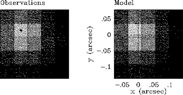
Figure 1: The final peak-up acquisition stage positions the 0.1-PAIR aperture at the points of a $5\times 5$ grid on the sky. The left panel shows the observed intensities in a grey-scale representation. The dot marks the grid point with the highest intensity, which is adopted by the telescope software as its estimate for the position of the galaxy center. The major axis of the galaxy lies along the $y$-axis. The right panel shows a model fit to the observations, based on the Lauer et al. (1992) cusp model for the M32 surface brightness, and the PSF and aperture size derived in Appendix A. The cross marks the position of the galaxy center in this best-fit model. The adopted position for the galaxy center is offset from the model position by (only) $(\Delta_{x},\Delta_{y})=(-0.010^{\prime\prime},0.015^{\prime\prime})$. Hence, the target acquisition was successful.

The observed intensities in the acquisition stages can be analyzed post facto, to determine the extent to which the acquisition was successful. Most important are the results of the fifth and final stage, in which the 0.1-PAIR aperture was sequentially positioned at the points of a $5\times 5$ grid on the sky, with spacing of $0.043^{\prime\prime}$ between the grid points. The left panel of Figure 1 shows a grey-scale representation of the observations. The solid dot marks the position with the highest intensity, which was adopted by the telescope software as its best estimate for the position of the galaxy center.

To model the observed intensities, the ‘cusp model’ for the unconvolved M32 surface brightness presented by Lauer et al. (1992) was used, which is based on pre-COSTAR HST/WFPC images. The point-spread-function (PSF) of the HST+FOS was approximated by a sum of Gaussians, as determined in Appendix A. The total magnitude at each grid point was calculated using the equations in the Appendix. The offset $(\Delta_{x},\Delta_{y})$ was varied to optimize the fit. The best fit is displayed in the right panel of Figure 1. It has $(\Delta_{x},\Delta_{y})=(-0.010^{\prime\prime},0.015^{\prime\prime})$, with a formal error in either coordinate (based on the chi-squared surface of the fit) of approximately 1 mas. The target acquisition was thus successful.

3.2 FOS image

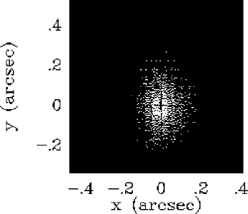
Figure 2: FOS image with overlaid contours of the central region of M32, taken at the end of the observations to verify the telescope pointing. Raw FOS images have very poor spatial resolution ($0.301^{\prime\prime}\times 1.291^{\prime\prime}$, i.e. similar in size to the image itself). The displayed image was obtained from the raw image through deconvolution. Features such as the deviations of the isophotes from ellipses are artifacts of this deconvolution, and should not be trusted. However, the galaxy center can be accurately determined (cross). The dot marks the position where the telescope thought the galaxy center would be, which is offset by $(\Delta_{x},\Delta_{y})=(-0.024^{\prime\prime},0.095^{\prime\prime})$ from the actual center. This indicates that pointing errors must have accumulated during the observations.

An FOS image of the central region of M32 was obtained in the final orbit of the observations. The telescope was commanded to position the upper ‘1.0-PAIR’ aperture, which has a nominal post-COSTAR size of $0.86^{\prime\prime}$ square, on the galaxy center, after which the intensity on the photocathode was scanned with the diode array of the detector (with no grating in the light path). The scan pattern was chosen to provide $0.038^{\prime\prime}\times 0.041^{\prime\prime}$ pixels. However, the spatial resolution of the image is poor, $0.301^{\prime\prime}\times 1.291^{\prime\prime}$, corresponding to the size of one FOS diode (Koratkar et al. 1994; Evans 1995b). The resolution can be improved by deconvolution. Figure 2 shows the result of Lucy deconvolving the raw image with a boxcar PSF with the size of one diode. The cross marks the galaxy center, while the dot marks the aperture center, i.e., the position where the telescope thought the galaxy center would be. The latter is offset from the actual galaxy center by $(\Delta_{x},\Delta_{y})=(-0.024^{\prime\prime},0.095^{\prime\prime})$ (with a formal error of 3 mas in each coordinate). This offset at the end of the observations is much larger than that achieved by the target acquisition. Hence, positional errors must have accumulated during the observations. The reason for this is not well understood. However, the most likely cause is a drift of the telescope pointing due to thermal effects related to the heating and cooling of the spacecraft and Fine Guidance Sensors (FGSs) during the 14.4 hours of the observations. Such thermal effects exist (Lupie, priv. comm.), but were not previously reported to complicate observations with the FOS (Keyes, priv. comm.).

3.3 Spectra

Nine spectra were taken. Those obtained with the 0.1-PAIR aperture are referred to as S1–S4, those obtained with the 0.25-PAIR aperture as L1–L5. Table 2 summarizes the observational setup for each spectrum. It also lists the position with respect to the galaxy center at which the telescope was instructed to place the aperture. These intended aperture placements are illustrated in the left panel of Figure 3.

In reality, the apertures were not placed exactly at their intended positions. The actual position is a sum of two vectors: (i) an intentional offset from the (telescope’s estimate of the) galaxy center (Table 2); and (ii) an unintentional offset $(\Delta_{x},\Delta_{y})$ of the telescope’s estimate of the galaxy center from the actual galaxy center. The intentional offsets are applied by slewing the telescope, which should be very precise ($\lesssim 1$ mas positional error). To determine the actual aperture positions one thus needs to know the offset $(\Delta_{x},\Delta_{y})$ for each observation. These can be determined by modeling the observed intensities of the spectra, which are listed in Table 3.

The spectra S1 and S2, taken in the subsequent orbits #3 and #4, were scheduled to have identical aperture positions (cf. Table 2). The same holds for the observations L4 and L5, taken in the subsequent orbits #8 and #9. In both cases, however, the observed intensities in the two spectra are significantly different. This indicates that the aperture positions must have changed (by $\sim 25$ mas, cf. Figure 4 below) between the orbits #3 and #4, and between the orbits #8 and #9. There was no motion of either the grating wheel or the aperture wheel of the instrument between the different observations. The guide star reacquisition at the beginning of each orbit is normally accurate to a few mas. Hence, the inferred pointing drifts are indeed most likely due to thermal effects on the FGS.

To proceed we make a number of simplifying assumptions about the offset $(\Delta_{x},\Delta_{y})$: (i) the offset for the first spectrum, S1, taken in orbit #3, was identical to the offset determined from the final peak-up stage (Figure 1), executed in orbit #2; (ii) the offset for the last spectrum, L5, taken in orbit #9, was identical to the offset determined from the FOS image (Figure 2), taken in that same orbit; (iii) the observations S2–S4, taken in orbits #4, #5 and #6, have a common offset; and (iv) the observations L1–L4, taken in orbits #7 and #8, have a common offset. These assumptions do not allow for positional errors between orbits #4 and #5, between orbits #5 and #6, and between orbits #7 and #8. Even though errors could have occurred, they are not required to fit the observed intensities. The assumptions do allow for an error between orbits #6 and #7, when the 0.1-PAIR aperture was replaced by the 0.25-PAIR aperture. This is because these apertures might not be exactly concentric on the aperture wheel (Evans et al. 1995), and because the motion of the aperture wheel might have a positional non-repeatability (Dahlem & Koratkar 1994).

With these assumptions, the offset $(\Delta_{x},\Delta_{y})$ can be determined for each observation by fitting to the observed intensities, using the Lauer et al. (1992) cusp model for the M32 surface brightness, and the aperture sizes and PSF determined in Appendix A. The results are displayed in Figure 4. The corresponding aperture placements for the individual spectra are listed in Table 3 and are displayed in the right panel of Figure 3. The fits to the intensities constrain only the absolute value of $\Delta_{x}$, and not its sign. This introduces an ambiguity for L1–L4, which was resolved by adopting the same sign for $\Delta_{x}$ as measured in Figure 2 (so as to minimize the size of the positional error between orbits #8 and #9). At the positions of the apertures (along the major axis), the surface brightness changes more rapidly along the $y$ direction than along the $x$-direction. Hence, the observed intensities constrain the $\Delta_{y}$ more tightly than the $\Delta_{x}$. Other model assumptions to fit the observed intensities were also studied. In all cases the results for $\Delta_{y}$ agreed to within a few mas, while the $\Delta_{x}$ could differ by as much as $0.02^{\prime\prime}$.

4 Data reduction

Most of the necessary data reduction steps are performed by the HST calibration ‘pipeline’. For the M32 data, three issues required additional attention: (i) wavelength calibration; (ii) absolute sensitivity calibration; and (iii) flat-fielding.

4.1 Wavelength calibration

The wavelength scale provided by the calibration pipeline is not accurate enough for our project. Arc lamp spectra were therefore obtained in each orbit during occultation. The emission line centers were determined, yielding for each arc spectrum $j$ and for each line $i$ with vacuum wavelength $\lambda_{{\rm vac},i}$, the observed wavelength $\lambda_{{\rm pipe},ij}$ on the scale provided by the calibration pipeline. Subsequently, the observed offsets $\Delta_{ij}\equiv\lambda_{{\rm pipe},ij}-\lambda_{{\rm vac},i}$ were fit as

$$\Delta_{ij}=D+P_{3}(\lambda_{{\rm vac},i})+d_{j}.$$ (1)

The constant offset $D$ is the result of non-repeatability in the FOS grating and aperture wheels, and was measured to be $6.17$Å. The third order polynomial $P_{3}$ with zero mean accounts for a slight ($|P_{3}|\lesssim 0.25$Å) non-linearity of the wavelength scale. The offsets $d_{j}$ account for constant shifts of the wavelength scale from orbit to orbit, mostly due to the ‘geo-magnetically induced image motion problem’ (Keyes et al. 1995). These shifts ranged between $\pm 0.18$Å, and could be determined with $0.02$Å ($\sim 1\>{\rm km}\,{\rm s}^{-1}$) accuracy.

The wavelength scale of the M32 spectra was corrected using the above fits to the arc spectra. An additional shift of $-0.769$Å was applied to correct for the fact that the light path for external targets differs from that for the internal arc lamp (Keyes et al. 1995). For each M32 spectrum the $d_{j}$ were used that was/were determined from the arc spectrum/spectra obtained immediately preceding or following the M32 spectrum. The fact that the arc spectra are never obtained completely simultaneously with galaxy spectra introduces a slight additional uncertainty. The cumulative uncertainty in the mean streaming velocities of the stars as a result of uncertainties in the wavelength scale is estimated to be $\lesssim 2\>{\rm km}\,{\rm s}^{-1}$. This is always smaller than the formal errors in these velocities as a result of photon noise (cf. Table 4 below).

After wavelength calibration (and absolute sensitivity calibration and flat-fielding as described below) the galaxy spectra were rebinned logarithmically in wavelength, as required for the stellar kinematical analysis. A scale of $57.9\>{\rm km}\,{\rm s}^{-1}/$pixel was used. The FOS is a photon counting detector, so the formal errors in the spectra follow directly from Poisson statistics. On average, the (logarithmic) rebinning decreases the formal errors, since it reduces the scatter between neighboring pixels. The decrease can be calculated for each pixel, and was taken into account in the subsequent analysis. The correlation between the errors in neighboring pixels induced by the rebinning was neglected.

4.2 Absolute sensitivity calibration

The calibration pipeline multiplies the observed count rate spectra by a so-called ‘inverse sensitivity file’ (IVS), to obtain fluxes in ${\rm erg}\,{\rm cm}^{-2}\,{\rm s}^{-1}\,$Å^-1. The pipeline IVS files contain a wavelength dependent aperture throughput correction, based on calibration observations of point sources. These, however, are not applicable to extended sources. Therefore, instead of the standard pipeline IVS file a more recent IVS file with no aperture throughput correction was used, provided to us by FOS Instrument Scientist Tony Keyes.

Each wavelength in the M32 spectra samples a slightly different region of the galaxy, because of the wavelength dependence of the PSF. This influences only the continuum slope of the spectra, because the PSF varies very slowly with wavelength. In the stellar kinematical analysis one is only interested in the absorption lines, which are not influenced. The underlying continuum is subtracted. Hence, no attempt was made to construct aperture throughput corrections. (In fact, this would require accurate knowledge of the wavelength dependence of the PSF, which is not readily available for the FOS; see Appendix A).

4.3 Flat-fielding

A G570H flat-field based on multiple 0.25-PAIR (upper) aperture observations of a star was used, as provided to us by Tony Keyes. No flat-fields obtained explicitly with the 0.1-PAIR (upper) aperture were available. A star illuminates the photocathode of the detector differently than an extended source. To test the appropriateness of the flat-field for the M32 data it was cross-correlated with the continuum subtracted normalized galaxy spectra. This yielded clear peaks, indicating that the flat-field and the M32 spectra share the same features (as they should). The peak was only $\sim$10% lower for the 0.1-PAIR spectra than for the 0.25-PAIR spectra. This indicates that the flat-field can be properly used for the 0.1-PAIR (upper) aperture as well, although a flat-field obtained specifically with that aperture would have been preferable. Shifts between the galaxy spectra and flat-field were identified from the positions of the cross-correlation peaks, and were corrected for (see also Kormendy et al. 1996a). The flat-fielding removes most of the pixel-to-pixel sensitivity variations, but some small residual variations might remain.

5 Line-spread-functions

The observed spectrum of a source is the convolution of its actual spectrum with the line-spread-function ${\rm LSF}(\lambda)$. The LSF can be written as the convolution of an ‘illumination function’ $B(\lambda)$ and an ‘instrumental broadening function’ $H(\lambda)$ (cf. Appendix B). The function $B(\lambda)$ is the normalized intensity distribution of the light that falls onto the grating. It depends on the target brightness and choice of aperture. The direction of dispersion is parallel to the $x$ direction. Hence, $B(\lambda)$ is the integral over the $y$ direction of the two-dimensional brightness distribution that falls onto the grating. For the PSF and aperture sizes derived in Appendix A, $B(\lambda)$ is given by equations (B3) and (B4) in Appendix B. It can be calculated for each observation upon substitution of the Lauer et al. (1992) cusp model for the M32 surface brightness, and the aperture positions in Table 3. The normalized function $H(\lambda)$ accounts for the instrumental broadening due to the grating and finite size of a detector diode (the resolution element). It was determined empirically from fits to the emission line shapes in the arc spectra, as discussed in Appendix B.

The LSF has zero mean if the galaxy light is distributed symmetrically within the aperture. This is not generally the case, because the aperture centers are not exactly at $x=0$ (Figure 3). Calculations show that the intensity weighted mean position is within $0.01^{\prime\prime}$ from the aperture center for all the observations. Nonetheless, there are noticeable wavelength shifts, because $0.01^{\prime\prime}$ projects onto $0.145$Å in the wavelength direction ($8.4\>{\rm km}\,{\rm s}^{-1}$ at 5170Å). Table 3 lists the LSF mean as calculated for each of the M32 spectra, both in Å and in $\>{\rm km}\,{\rm s}^{-1}$ at 5170Å. Errors in these values due to errors in the aperture positions do not exceed 0.04Å ($2\>{\rm km}\,{\rm s}^{-1}$ at 5170Å).

The width and shape of the LSF are determined mainly by the aperture size. The calculated LSFs for all the M32 spectra are shown in Figure 5. The LSF shapes for the 0.1-PAIR observations are very similar to each other, as are the LSF shapes for the 0.25-PAIR observations. The shapes are also similar to the emission line shapes observed directly in arc spectra (Figure 9). The 0.25-PAIR LSF can be well approximated by convolving the 0.1-PAIR LSF by a Gaussian with a dispersion of $1.14$Å ($66\>{\rm km}\,{\rm s}^{-1}$ at 5170Å), as illustrated by the dotted curve in Figure 5.

The best-fitting Gaussian to the 0.1-PAIR LSF has a dispersion of $1.65$Å ($96\>{\rm km}\,{\rm s}^{-1}$ at 5170Å). For the 0.25-PAIR LSF it has a dispersion of $1.98$Å ($115\>{\rm km}\,{\rm s}^{-1}$ at 5170Å). However, these numbers are of limited use in characterizing the LSFs, since these have noticeably broader wings than a Gaussian.

6 Template spectrum

For stellar kinematical analysis a template spectrum is needed to compare the M32 spectra to. To avoid systematic errors it is important to minimize template mismatching. This is best done by constructing a composite template which contains an appropriate mix of spectral types. Observing template stars with the HST is inefficient and time consuming (mainly because of the lengthy target acquisitions that are required). To date less than a handful different template stars have been observed with the HST, all of similar spectral type. These HST spectra are insufficient to construct an optimal template. A ground-based template library of spectra of 27 stars of different spectral types was therefore used, obtained in February 1990 by M. Franx at the 4m telescope of the KPNO with the RC Spectrograph (as discussed previously by van der Marel & Franx 1993). The LSF of these spectra is approximately Gaussian with a dispersion of $1.22$Å ($71\>{\rm km}\,{\rm s}^{-1}$ at 5170Å). The spectra cover the spectral range from 4836Å to 5547Å, centered on the Mg b triplet at $\sim 5170$Å. This is the most useful wavelength range for stellar kinematical analysis, so it is no drawback that this range is smaller than the full range covered by the FOS G570H grating.

The stellar spectra were similarly rebinned logarithmically as the galaxy spectra, and shifted to a common velocity. No attempt was made to construct a different composite template for each M32 spectrum (which is reasonable, given that there are no strong color gradients in the central arcsec; Lugger et al. 1992). Instead, the best fit was sought to a grand-total M32 spectrum, constructed by summing the HST spectra. The resulting composite template is a weighted mix of the individual templates, with the weights determined using the method outlined in Appendix A.3 of van der Marel (1994a). The mix contains giants, sub-giants and dwarfs of spectral types G and K.

The composite template is used in the remainder of the paper. However, other templates were studied as well. For example, a stellar kinematical analysis was performed with a K-star template spectrum obtained from the HST Data Archive, taken with the FOS circular 0.3 aperture ($0.26^{\prime\prime}$ diameter) by H. Ford and collaborators before the installation of COSTAR. This template provides a poor fit to the spectrum of M32. Nonetheless, the stellar kinematical properties inferred with this template were found to be consistent with those derived using the composite template.

7 Kinematical analysis

7.1 Description

The stellar kinematical analysis was performed with the method presented in van der Marel (1994a). It fits the convolution of a parametrized velocity profile and a template spectrum to a galaxy spectrum in pixel space, using chi-squared minimization. The formal errors in the fit parameters follow from the shape of the chi-squared surface near its minimum. The method has been well tested, and its results agree with those from other methods for extracting stellar kinematics from galaxy spectra. Deviations of the line-of-sight velocity profiles from Gaussians contain useful information on the dynamical structure of galaxies. Unfortunately, the velocity resolution of the FOS is too poor to extract any reliable velocity profile shape information from the M32 data. The analysis was therefore restricted to Gaussian velocity profile fits.

Data obtained with the FOS is time resolved. The red side detector reads and stores the data every $\sim 2$ minutes. Between 6 and 20 spectra were therefore available per aperture position. The aperture positions for the observations L4 and L5 differ by $\sim 0.024^{\prime\prime}$, but both are at a distance of $\sim 0.5^{\prime\prime}$ from the galaxy center, where kinematical gradients are small. In the kinematical analysis L4 and L5 were therefore treated as a single observation, referred to as L45. Especially for the 0.1-PAIR observations, the signal-to-noise ratio (S/N) of the individual read-outs is low. Individual read-outs for a given aperture position were therefore added to achieve an average S/N of $\sim 10$ per (logarithmically rebinned) pixel. This resulted in 4 independent spectra for each of the observations S1–S4 with the 0.1-PAIR aperture, and between 9 and 11 independent spectra for the observations L1, L2, L3 and L45 with the 0.25-PAIR aperture. A stellar kinematical analysis was performed on each of these spectra. The kinematical results for each aperture position were then averaged together, weighted with the errors. It was found that this yields slightly more accurate results than a kinematical analysis of the sum of the individual spectra for a given aperture position. No systematic trends with time in the orbit were found in the kinematical results.

The stellar kinematical analysis was performed over the wavelength range 4859–5520Å. Regions influenced by so-called ‘noisy’ diodes were masked. The fit to the galaxy spectrum includes a low order polynomial to account for continuum differences between the galaxy and template spectrum. This polynomial is fit simultaneously with the velocity profile. The parameters of the best-fitting velocity profile are virtually independent of the choice of polynomial order. A polynomial of order 5 was used.

7.2 Corrections

The mean velocity and velocity dispersion of the best-fitting Gaussian velocity profiles must be corrected for instrumental effects. The mean velocity is biased because the LSF mean is non-zero. This bias is removed by subtracting the corrections $\Delta V_{\rm LSF}$ listed in Table 3. These were calculated for the wavelength 5170Å of the Mg b triplet, but the wavelength dependence of the velocity corrections over the fit range is negligible ($\lesssim 0.4\>{\rm km}\,{\rm s}^{-1}$ in absolute value). Further, to obtain velocities in the M32 frame one must subtract a constant offset, determined by the difference between the systemic velocity of M32 and the template velocity. These were not known accurately enough to determine the offset directly, and it was therefore estimated from the data itself. Somewhat arbitrarily, it was fixed to the intercept of the best least-squares fit line in a plot (see Figure 6c below) of rotation versus position $y$ along the M32 major axis for the observations S4, S1 and S2 (for which $y=-0.046^{\prime\prime}$, $0.015^{\prime\prime}$ and $0.040^{\prime\prime}$, respectively).

The velocity dispersions ${\tilde{\sigma}}$ of the best-fitting Gaussians must be corrected for differences in the LSFs of the template and galaxy spectra. For this it is useful to consider not the observed dispersions themselves, but rather differences in the observed dispersions between two observations. Let ${\tilde{\sigma}}_{\rm A}$ and ${\tilde{\sigma}}_{\rm B}$ be the best-fitting dispersions for observations at positions A and B. Assume that the LSF of observation B can be obtained from the LSF of observation A through convolution with a Gaussian of dispersion $S_{\rm LSF}$. The difference between the actual dispersions at positions A and B can then be estimated as:

$$\sigma_{\rm A}^{2}-\sigma_{\rm B}^{2}={\tilde{\sigma}}_{\rm A}^{2}-{\tilde{\sigma}}_{\rm B}^{2}+S_{\rm LSF}^{2},$$ (2)

(which uses the fact that the convolution of two Gaussians is again a Gaussian, the dispersion of which is the RMS sum of the input dispersions). This approach has two important advantages. First, the LSF of the template influences the kinematical analysis at points A and B in the same way, so it does not enter into $\sigma_{\rm A}^{2}-\sigma_{\rm B}^{2}$. Second, the differences in the LSFs for the HST observations can in fact to good approximation be accounted for by convolution with a Gaussian (cf. Figure 5). One does not have to assume that the LSFs themselves are Gaussian, which would be a poor approximation.

In the following, the observation L45 at $\sim 0.5^{\prime\prime}$ from the galaxy center is used as ‘reference point’. Equation (2) then yields

$$\sigma^{2}-\sigma_{\rm L45}^{2}={\tilde{\sigma}}^{2}-{\tilde{\sigma}}_{\rm L45}^{2}+S_{\rm LSF}^{2},$$ (3)

where $S_{\rm LSF}=0$ for an observation with the 0.25-PAIR aperture, and $S_{\rm LSF}=66.2\>{\rm km}\,{\rm s}^{-1}$ for an observation with the 0.1-PAIR (based on the results of Section 5). The latter value was calculated for the wavelength 5170Å of the Mg b triplet, which is roughly at the center of the fit range. The actual value of $S_{\rm LSF}$ varies from $62.0$ to $70.4\>{\rm km}\,{\rm s}^{-1}$ over the fit range, which can be taken into account by assigning a ‘formal’ error of $4.2\>{\rm km}\,{\rm s}^{-1}$ to $S_{\rm LSF}$. Equation (3) can be used to estimate the stellar velocity dispersion $\sigma$ for any of the observations S1–S4 and L1–L3, if one assumes that the dispersion $\sigma_{\rm L45}$ at the position of observation L45 is known a priori. At $\sim 0.5^{\prime\prime}$ along the major axis one is beyond the region most influenced by seeing in ground-based data. Based on the data of van der Marel et al. (1994a) and Bender, Kormendy & Dehnen (1996) it was assumed that $\sigma_{\rm L45}=70\pm 5\>{\rm km}\,{\rm s}^{-1}$ (see Figure 6d below).

It is demonstrated in Appendix C that the velocity dispersions thus obtained have no systematic biases, and that even velocity dispersions as small as $\sim 50\>{\rm km}\,{\rm s}^{-1}$ can be measured reliably, in spite of the large FOS instrumental dispersion of $\gtrsim 100\>{\rm km}\,{\rm s}^{-1}$. The formal errors in dispersions $\sigma$ obtained from equation (3) follow from the errors in ${\tilde{\sigma}}$, ${\tilde{\sigma}}_{\rm L45}$, $\sigma_{\rm L45}$ and $S_{\rm LSF}^{2}$ using a standard first order error analysis. Systematic errors due to template mismatching are not likely to exceed a few $\>{\rm km}\,{\rm s}^{-1}$, and are smaller than the formal errors in the measurements.

7.3 Results

Table 4 lists the line strengths, rotation velocities and velocity dispersions, after correction for all instrumental effects. These results are discussed below. Figure 6 displays the results as function of the position $y$ of the aperture center along the M32 major axis. The best spatial resolution ground-based M32 data are also shown. These are the data from van der Marel et al. (1994a) obtained at the William Herschel Telescope (WHT), and those of Bender, Kormendy & Dehnen (1996) obtained at the Canada France Hawaii Telescope (CFHT). A comparison of these ground-based data to older (lower spatial resolution) ground-based data can be found in Kormendy & Richstone (1995).

The spatial resolution for each of the observations in Figure 6 is characterized by a convolution kernel, which results from the PSF and finite aperture size (for ground-based long-slit data the effective aperture is the spatial CCD pixel size by the slit width). The top left-panel illustrates the difference in spatial resolution between the data sets. It displays the projection of the convolution kernel along the M32 minor axis, i.e., the probability $P(y)$ that a photon observed in a given aperture was emitted at distance $y$ from the center of that aperture, measured along the M32 major axis. These probability distributions have FWHM values of $0.102^{\prime\prime}$, $0.203^{\prime\prime}$, $0.541^{\prime\prime}$ and $0.911^{\prime\prime}$, for the HST/FOS/0.1-PAIR, HST/FOS/0.25-PAIR, CFHT and WHT data, respectively. The HST data therefore provide a factor 5 increase in spatial resolution over even the best available ground-based data.

7.3.1 Line strengths

The line strengths shown in Figure 6b were normalized to an average of unity (line strengths are measured with respect to the template spectrum, and are hence on an arbitrary scale). There is no obvious trend with radius. The observations with the 0.1-PAIR aperture closest to the nucleus have relatively low line strength, but this is unlikely to be real. Metallicities and line strengths generally increase towards the centers of galaxies. The observed low values could be an artifact due to the presence of a black hole. The stars that move rapidly near the black hole produce broad velocity profile wings. These can be mistaken for an enhanced continuum, which causes the line strength to be underestimated (van der Marel 1994b). The broad-band colors of M32 are constant in the central arcsec (Lugger et al. 1992). The true line strengths in the central $0.5^{\prime\prime}$ covered by the HST observations are therefore probably also close to constant.

The observed line strengths have a sizable RMS scatter of $\sim 0.055$. This exceeds the formal errors, which are on average $\sim 0.03$. The measurements are therefore not statistically consistent with a constant line strength (as is confirmed by a chi-squared test). The scatter in the observed line strengths could be the result of minor inaccuracies in the data, such as unidentified bad pixels or flat-field errors, or it could be real, and due to shot noise in the contributions from individual stars. The total V-band luminosity inside the aperture varies from $3\times 10^{4}L_{\odot}$ (for observation S3) to $2.5\times 10^{5}L_{\odot}$ (for observation L3). Most of the observed light comes from giants, some of which can be as luminous as $10^{3}L_{\odot}$ (Freedman 1989). The luminosity of a ‘typical’ giant as measured from surface brightness fluctuations (Tonry, Ajhar & Luppino 1990) is $\sim 10^{1.6}L_{\odot}$. This implies that there are $N=10^{3-4}$ typical stars in each HST aperture. Therefore, $\sqrt{N}$ fluctuations can be of order a few percent of the intrinsic line strength differences between stars.

7.3.2 Kinematics

Figure 6c shows the rotation velocities. The HST rotation curve is smooth. It is significantly steeper in the central $0.2^{\prime\prime}$ than seen in the ground-based data, consistent with the presence of a central black hole. The rotation velocity is observed to be $\sim 30\>{\rm km}\,{\rm s}^{-1}$ at $0.1^{\prime\prime}$ from the nucleus. This is roughly twice the value measured from the ground at this distance.

The scatter in the line strength measurements (Figure 6b) induces scatter in the velocity dispersion measurements, because the velocity dispersion and line strength of a Gaussian fit are statistically correlated. Tests indicate that a line strength error $\Delta\gamma$ induces an error $\Delta\sigma=1.4\,(\Delta\gamma/0.01)\>{\rm km}\,{\rm s}^{-1}$ in the velocity dispersion. Rotation velocity measurements are not influenced. To avoid unwanted errors in the velocity dispersion measurements, they were determined by fitting Gaussian velocity profiles to the data while keeping the line strength constant to the mean of the measurements in Figure 6b. This yields velocity dispersions that differ only at the $\lesssim 10\>{\rm km}\,{\rm s}^{-1}$ level from those obtained by Gaussian fits with variable line strength, so the main results do not depend on this correction.

Figure 6d shows the resulting velocity dispersions. The dispersion measured with the 0.1-PAIR aperture closest to the nucleus is $156\pm 10\>{\rm km}\,{\rm s}^{-1}$. The profile of the velocity dispersion with radius is smooth, with the exception of the measurement $\sigma=96\pm 10\>{\rm km}\,{\rm s}^{-1}$ from observation S2, which is significantly lower than that for the other observations in the central $0.1^{\prime\prime}$. We doubt the reality of this, but have not been able to attribute it to any known instrumental effect. The average of the four dispersion measurements inside $0.1^{\prime\prime}$ is $126\>{\rm km}\,{\rm s}^{-1}$, with a RMS scatter of $21\>{\rm km}\,{\rm s}^{-1}$. Hence, the central velocity dispersion is definitely higher than the 85–95$\>{\rm km}\,{\rm s}^{-1}$ determined from ground-based measurements. It thus appears that a Keplerian increase in the velocity dispersion close to the center of M32 has been resolved.

The difference in the dispersions measured for observations S1 and S2, which were obtained with the same aperture at similar positions, indicates that uncertainties in the velocity dispersions are dominated by systematic errors, rather than Poisson noise. Systematic errors in the rotation velocity measurements are believed to be much smaller, primarily because these are less sensitive to the poor instrumental resolution of the FOS. Either way, the data clearly imply that the dispersion in the central $0.1^{\prime\prime}$ is higher than measured from ground-based data. Whether the nuclear dispersion seen through a small aperture is indeed as high as $156\>{\rm km}\,{\rm s}^{-1}$ should await verification by observations with the future HST spectrograph STIS.

8 Discussion

HST/FOS spectra were obtained through small apertures centered on the nuclear region and major axis of M32. Kinematical analysis of these data is more complicated than it is for ground-based data: the FOS is a low-resolution spectrograph, and is not particularly well suited for dynamical studies of low-dispersion objects such as M32. One of the main results of this paper is therefore that stellar kinematical quantities can in fact be determined from the data, provided that a detailed study is made of various technical issues, including: calibration and modeling of the FOS aperture sizes, PSF and LSFs, determination of the aperture positions from the data, accurate wavelength calibration, template matching, and corrections for instrumental resolution.

The resulting kinematical quantities are displayed in Figure 6. The main result is that in the central $0.1^{\prime\prime}$ the M32 rotation curve is significantly steeper, and the velocity dispersion significantly higher, than measured from even the highest resolution ground-based data. These observational results are robust. They do not depend critically on the corrections made in the analysis; even a rough analysis without any template matching and corrections for instrumental effects shows these main features. The results are exactly what would be expected if M32 does indeed have a massive dark object in its nucleus, as suggested previously on the basis of ground-based data. In the companion papers in this series (van der Marel et al. 1997a,b; Cretton et al. 1997) we construct dynamical models to address the presence of such a dark object quantitatively. We also address the question whether the dark object has to be a black hole, or whether plausible alternatives still exist.

Appendix A Point-spread-function and aperture sizes

Some calibrations exist of the HST+FOS PSFs and LSFs (Koratkar 1996) and of the FOS aperture sizes (Evans et al. 1995), but these are too crude for the purposes of this paper. To obtain more accurate calibrations we present detailed models for the calibration observations obtained by Evans (1995a) after the installation of COSTAR. He centered a star in FOS apertures, and stepped the star across each aperture in the FOS $x$ and $y$ directions, respectively. At each step the total intensity was measured. Here the results are considered for the FOS red detector with three apertures: the square upper aperture of the 0.1-PAIR, the square upper aperture of the 0.25-PAIR, and the circular 1.0. The names of these apertures are based on their size in arcsec, before the installation of COSTAR. Their nominal post-COSTAR sizes are smaller by a factor $\sim 0.86$. Figure 7 shows for each aperture the observed intensity as function of distance from the aperture center, normalized by the observed intensity with the star at the center of the circular 1.0 aperture. The aperture length or diameter is easily determined from these data for apertures much larger than the PSF core: it is then twice the radius at which the intensity has fallen to 50% of its central value. This was used by Evans et al. (1995) to estimate the size of all FOS apertures. Although this is reasonable for the larger apertures, it is not for the smaller apertures. For those a more careful analysis is required, in which the aperture sizes and PSF are fitted to the data simultaneously.

For a target with surface brightness $S(x,y)$, the intensity $I$ observed through an aperture centered on $(x,y)$ is

$$I(x,y)=\int_{-\infty}^{\infty}\int_{-\infty}^{\infty}S(x^{\prime},y^{\prime})\>K(x^{\prime}-x,y^{\prime}-y)\>dx^{\prime}\>dy^{\prime},$$ (A1)

where $K(x,y)$ is a convolution kernel that depends on the PSF and the aperture size and geometry. The PSF is assumed to be a circularly symmetric sum of Gaussians,

$${\rm PSF}(r)=\sum_{i=1}^{N}\>{{\gamma_{i}}\over{2\pi\sigma_{i}^{2}}}\>\exp\left[-{\textstyle{1\over 2}}({\textstyle{r\over\sigma_{i}}})^{2}\right],$$ (A2)

where the $\gamma_{i}$ must satisfy $\sum_{i=1}^{N}{\gamma_{i}}=1$. For a perfectly rectangular aperture with sides $A_{x}$ and $A_{y}$ the convolution kernel is then

$$K(x,y)=\sum_{i=1}^{N}\>{{\gamma_{i}}\over 4}\>\left\{\mathop{\rm erf}\nolimits\left[{\textstyle{x+(A_{x}/2)\over\sqrt{2}\>\sigma_{i}}}\right]-\mathop{\rm erf}\nolimits\left[{\textstyle{x-(A_{x}/2)\over\sqrt{2}\>\sigma_{i}}}\right]\right\}\>\left\{\mathop{\rm erf}\nolimits\left[{\textstyle{y+(A_{y}/2)\over\sqrt{2}\>\sigma_{i}}}\right]-\mathop{\rm erf}\nolimits\left[{\textstyle{y-(A_{y}/2)\over\sqrt{2}\>\sigma_{i}}}\right]\right\},$$ (A3)

while for a perfectly circular aperture with diameter $D$ it is

$$K(\rho\cos\theta,\rho\sin\theta)=\sum_{i=1}^{N}\>{{\gamma_{i}}\over{\sigma_{i}^{2}}}\exp\left[-{\textstyle{1\over 2}}({\textstyle{\rho\over\sigma_{i}}})^{2}\right]\int_{0}^{D/2}\exp\left[-{\textstyle{1\over 2}}({\textstyle{r\over\sigma_{i}}})^{2}\right]\>I_{0}({\textstyle{r\rho\over\sigma_{i}^{2}}})\>r\>dr,$$ (A4)

(van der Marel 1995). The function ${\rm erf}(t)$ is the error function and $I_{0}(t)$ is a Bessel function.

This model was used to fit the data in Figure 7. For a point source at $(x_{0},y_{0})$, the intensity observed through an aperture centered at the origin is simply $K(x_{0},y_{0})$. The solid curves in the figure show the best chi-squared fit to the data for a PSF that is a sum of three Gaussians. The aperture sizes were treated as free parameters. The square apertures were assumed to have equal sizes in the $x$ and $y$ directions. The model was forced to fit 2 additional constraints, obtained from theoretical modeling (as quoted in Keyes et al. 1995): (i) the throughput (for a centered point source) of the circular 1.0 aperture is $0.96$ times that of a rectangular aperture of size $3.7^{\prime\prime}\times 1.3^{\prime\prime}$; and (ii) the absolute throughput of the $3.7^{\prime\prime}\times 1.3^{\prime\prime}$ aperture is $0.975$. The best-fitting model parameters are listed in Table 5. The fit is robust, in spite of the fact that the model parameters are highly correlated. In particular: (i) no good fit can be obtained if the aperture sizes are held fixed to their nominal post-COSTAR values (which are $0.086^{\prime\prime}$ square, $0.215^{\prime\prime}$ square, and $0.86^{\prime\prime}$ circular, respectively); and (ii) the fit does not improve significantly if the number of Gaussians in the PSF is increased. The formal errors in the best fit parameters are $0.01$ for the $\gamma_{i}$, and $2$% for the $\sigma_{i}$ and aperture sizes. These numbers are not too meaningful, however, because systematic errors probably exceed the formal errors.

Figure 8 shows the PSF for the best fit, and the encircled flux curve $E(r)$. The latter is given by

$$E(r)\>\equiv\>\int_{0}^{r}{\rm PSF}(r^{\prime})\>2\pi r^{\prime}\>dr^{\prime}\>=\>1-\sum_{i=1}^{N}{\gamma_{i}}\>\exp\left[-{\textstyle{1\over 2}}({\textstyle{r\over\sigma_{i}}})^{2}\right].$$ (A5)

The PSF has 73% of the light within a circle of radius $0.1^{\prime\prime}$. This is smaller than the 84% measured from star images at visual wavelengths obtained with the FOC, but larger than the 65% measured with the WFPC2 (which suffers from additional pixel scattering). It should be noted that the PSF derived here pertains only to the upper position of the square paired FOS apertures. The aperture transmissions, and thus the PSF, are somewhat different at the lower positions of the square paired apertures (Evans 1995a).

The above analysis ignores the effects of diffraction at the aperture edges. The derived aperture sizes are therefore not the geometrical apertures sizes. This might explain why the derived sizes are smaller than the nominal post-COSTAR sizes. Non-circularly symmetric features in the PSF are also ignored. Such features might in fact be present, given that the results of scanning a star across the aperture in the $x$ and $y$ directions differ slightly (Figure 7). Either way, both the aperture sizes and the PSF enter into the data analysis only through the convolution kernels $K(x,y)$. These kernels are adequately fit by the model, independent of whether or not the aperture sizes and PSF of the model are unbiased estimates of their true values.

The observations in Figure 7 were derived from so-called ‘white light’ images, i.e., with no grating in the light path. The PSF with the parameters of Table 5 is therefore an average over all wavelengths to which the detector is sensitive. The M32 observations were obtained with the G570H grating. Observations with this grating (Bohlin & Colina 1995) show fractional throughputs for centered point sources that are larger by a few percent than those in Figure 7. This indicates that the core of the PSF for the G570H grating might be $\sim 15$% smaller than that of the PSF derived here. On the other hand, in fitting the M32 peak-up acquisition observations (Section 3.1) by convolving the Lauer et al. (1992) cusp model for the M32 surface brightness, it was found that the chi-squared of the fit could be improved by increasing the width of the PSF core by $\sim 15$%. This could mean that the PSF does in fact have a broader core than derived here, or alternatively, that the Lauer et al. model, based on WFPC1 measurements, is not a perfectly adequate representation of the M32 surface brightness in the central $0.1^{\prime\prime}$. In the absence of theoretical constraints on the wavelength dependence of the PSF from accurate wavefront modeling, it was decided not to make any corrections to the PSF derived from the white light images (Table 5). The PSF remains somewhat uncertain, but it was verified that changes in the PSF core width between $-20$% and 20% do not change any of the major conclusions of our paper(s).

Appendix B Line-spread-function

The observed spectrum $O(\lambda)$ of a source is the convolution of its actual spectrum $S(\lambda)$ with the line-spread-function ${\rm LSF}(\lambda)$,

$$O(\lambda)=\int_{-\infty}^{\infty}d\lambda^{\prime}\>S(\lambda^{\prime})\>{\rm LSF}(\lambda-\lambda^{\prime}).$$ (B1)

The LSF can be written as the convolution

$${\rm LSF}(\lambda)=\int_{-\infty}^{\infty}d\lambda^{\prime}\>B(\lambda^{\prime})\>H(\lambda-\lambda^{\prime}),$$ (B2)

where the ‘illumination function’ $B(\lambda)$ is the normalized intensity distribution of the light that falls onto the grating, and the normalized ‘instrumental broadening function’ $H(\lambda)$ accounts for the broadening due to the grating and the detector.

The $(x,y)$ coordinate system is defined such that the $x$ direction is parallel to the direction of dispersion. The function $B(\lambda)$ is therefore proportional to the integral over the $y$ direction of the two-dimensional brightness distribution that falls onto the grating. All the light in the aperture is detected, since the apertures used for the observations are smaller than the $y$-size of the diode array of the detector ($1.29^{\prime\prime}$). For the case of observations of a target with surface brightness $S(x,y)$ through an aperture centered on position $(x_{0},y_{0})$,

$$B(\lambda)={1\over{I(x_{0},y_{0})}}\int_{-\infty}^{\infty}\int_{-\infty}^{\infty}S(x^{\prime},y^{\prime})\>{\cal K}(x^{\prime}-x_{0},y^{\prime}-y_{0};x)\>dx^{\prime}\>dy^{\prime},$$ (B3)

where $I(x_{0},y_{0})$ is defined in equation (A1), and ${\cal K}(x^{\prime},y^{\prime};x)$ is a convolution kernel that depends on the PSF and the aperture size and geometry. For the G570H grating the wavelength $\lambda$ is related to the position $x$ according to $\lambda=14.489\>$(x/arcsec) Å. If the aperture is rectangular of size $A_{x}\times A_{y}$, and the PSF is as given in equation (A2), then

$${\cal K}(x^{\prime},y^{\prime};x)=\left\{\begin{array}[]{ll}\sum_{i=1}^{N}\>{{\gamma_{i}}\over{\sqrt{8\pi}\>\sigma_{i}}}\>\exp[-{1\over 2}({{x^{\prime}-x}\over{\sigma_{i}}})^{2}]\>\left\{\mathop{\rm erf}\nolimits\left[{{y^{\prime}+(A_{y}/2)}\over{\sqrt{2}\>\sigma_{i}}}\right]-\mathop{\rm erf}\nolimits\left[{{y^{\prime}-(A_{y}/2)}\over{\sqrt{2}\>\sigma_{i}}}\right]\right\},&\quad|x|\leq{{A_{x}}\over 2};\\ 0,&\quad|x|>{{A_{x}}\over 2}.\end{array}\right.$$ (B4)

The grating disperses the image of the aperture onto the photocathode of the detector, which is scanned using an array of diodes. A simple model for the instrumental broadening function $H(\lambda)$ is therefore:

$$H(\lambda)=\int_{-\infty}^{\infty}d\lambda^{\prime}\>D(\lambda^{\prime})\>G(\lambda-\lambda^{\prime}),$$ (B5)

where $D(\lambda)$ is the normalized response function of a detector diode and $G(\lambda)$ is the normalized broadening function of the grating. Let $D(\lambda)$ be a top-hat function with full width $d_{x}$, and let the grating broadening function be $G(\lambda)=(1/w)f(\lambda/w)$, where $f$ is a normalized function, and $w$ is a free parameter that measures the width of $G$. The notation

$$F^{(1)}(t)=\int f(t)\>dt,\qquad F^{(2)}(t)=\int F^{(1)}(t)\>dt,$$ (B6)

is used for the primitives of $f$. The function $H$ is then

$$H(\lambda)={\textstyle{1\over d_{x}}}\sum_{i=1}^{2}(-1)^{i}F^{(1)}(t_{i}),\qquad t_{i}\equiv{\textstyle{1\over w}}[\lambda+(-1)^{i}{\textstyle{d_{x}\over 2}}].$$ (B7)

It can be determined empirically by fitting to the emission lines in the arc spectra. If the arc lamp illuminates the aperture homogeneously, then $B(\lambda)$ is a normalized top-hat function of full width $A_{x}$. For an emission line that is intrinsically a delta-function at $\lambda_{0}$, the observed line shape will be

$$O_{\rm arc}(\lambda)={\textstyle{w\over A_{x}d_{x}}}\sum_{i=1}^{2}\sum_{j=1}^{2}(-1)^{i+j}F^{(2)}(t_{ij}),\qquad t_{ij}\equiv{\textstyle{1\over w}}[\lambda-\lambda_{0}+(-1)^{i}{\textstyle{A_{x}\over 2}}+(-1)^{j}{\textstyle{d_{x}\over 2}}].$$ (B8)

Several functional forms were considered for $f$. A Gaussian did not yield good fits to the observed line shapes. Satisfactory results were obtained with a Lorentzian, for which

$$f(t)={\textstyle{1\over\pi(1+t^{2})}},\qquad F^{(1)}(t)={\textstyle{1\over\pi}}\arctan t,\qquad F^{(2)}(t)={\textstyle{1\over\pi}}[t\arctan t-{\textstyle{1\over 2}}\ln(1+t^{2})].$$ (B9)

With this choice, the function $H$ has two parameters, $w$ and $d_{x}$. The best fit is generally attained for values of $d_{x}$ that differ from the actual size of one diode, which is $4.36$Å for the G570H grating. This probably indicates that the true diode response function is not a perfect top-hat. However, this does not invalidate the model. One is interested only in a fit to the function $H(\lambda)$, not in a determination of either $D(\lambda)$ or $G(\lambda)$. Therefore, both $w$ and $d_{x}$ are treated as free fitting parameters.

The best fits were determined to the emission line shapes in arc spectra obtained with the 0.1-PAIR and the 0.25-PAIR apertures, while keeping the values of $A_{x}$ fixed to their values in Table 5. Figure 9 shows the fits to the arc lines and the best-fitting function $H$. No evidence was found for a wavelength dependence of the LSF over the wavelength range covered by the grating. The best-fit parameters are: $w=0.595\pm 0.02$Å and $d_{x}=3.807\pm 0.02$Å for the 0.1-PAIR aperture, and $w=0.816\pm 0.04$Å and $d_{x}=3.904\pm 0.04$Å for the 0.25-PAIR aperture. Hence, the function $H(\lambda)$ is broader for the 0.25-PAIR aperture than for the 0.1-PAIR. The difference is too large to be attributed to small errors in the assumed aperture sizes. Hence, the instrumental broadening is more complicated in reality than in our simplified model, in which one would have expected $H(\lambda)$ to be independent of the aperture size. However, the only important point for the interpretation of the M32 spectra is that an accurate empirical description of the LSF is available. The fits in Figure 9 suggest that the model is satisfactory for this purpose.

Appendix C Velocity dispersion tests

C.1 Simulated galaxy spectra

Tests with artificial galaxy spectra were performed to determine whether systematic biases could be present in the velocity dispersion measurements. Artificial galaxy spectra were created from each of the 27 stellar spectra in the template library, by broadening them with Gaussian velocity profiles with dispersions $\sigma_{\rm in}$. Twenty copies were made of each broadened template, and noise was added to yield a S/N of 10 per pixel. A stellar kinematical analysis was then performed on each copy, using the composite spectrum discussed in Section 6 as template. The twenty velocity dispersion measurements where then averaged to yield an output velocity dispersion $\sigma_{\rm out}$.

Figure 10 plots $\sigma_{\rm out}$ as function of $\sigma_{\rm in}$ for each of the input spectra. The results lie closely along the line $\sigma_{\rm out}=\sigma_{\rm in}$. The minor deviations can be attributed entirely to the template mismatch in the simulations (the input stellar spectra are giants, sub-giants and dwarfs of spectral types G, K and M). At dispersions below $\sim 50\>{\rm km}\,{\rm s}^{-1}$ there is some tendency for the dispersion to be underestimated. However, for the M32 observations one is always in the situation where the difference in dispersion between the galaxy and template spectrum is $\gtrsim 100\>{\rm km}\,{\rm s}^{-1}$ (because the LSF of the galaxy spectra is broader than that of the template, in addition to the kinematical Doppler broadening). At these dispersions there are no significant biases in the results of the kinematical analysis, but only small ($\lesssim 5\>{\rm km}\,{\rm s}^{-1}$) errors due to template mismatching. These errors are nearly independent of the velocity dispersion. Since the approach used in this paper for determining velocity dispersions relies on differences between velocity dispersion measurements at different positions, it is expected that even these small errors largely cancel out.

C.2 Consistency check

A crude consistency check on our approach for determining velocity dispersions can be obtained by making the (poor) assumption that the LSFs of both the galaxy and template spectra are Gaussian, with dispersions $\sigma_{\rm LSF,t}$ and $\sigma_{\rm LSF,g}$, respectively. The stellar velocity dispersion $\sigma$ then follows from the dispersion ${{\tilde{\sigma}}}$ obtained by fitting to the galaxy spectrum, according to:

$$\sigma^{2}={\tilde{\sigma}}^{2}+\sigma_{\rm LSF,t}^{2}-\sigma_{\rm LSF,g}^{2}.$$ (C1)

For the observation L45 the dispersion measured directly from the spectra is ${\tilde{\sigma}}=111\pm 4\>{\rm km}\,{\rm s}^{-1}$. Upon substitution in equation (C1) of $\sigma_{\rm LSF,t}=71\>{\rm km}\,{\rm s}^{-1}$ (cf. Section 6), and $\sigma_{\rm LSF,g}=115\>{\rm km}\,{\rm s}^{-1}$ (cf. Section 5) one obtains the estimate $\sigma=63\pm 7\>{\rm km}\,{\rm s}^{-1}$ for the stellar velocity dispersion at $\sim 0.5^{\prime\prime}$ along the M32 major axis. This agrees reasonably well with the value of $\sigma=70\pm 5\>{\rm km}\,{\rm s}^{-1}$ adopted in Section 7.2 on the basis of ground-based measurements. This confirms the result of Appendix C.1 that there are no systematic biases in the velocity dispersion measurements from the spectra, and that the differences in the LSFs of the template and galaxy spectra can be fully corrected for.

Figure 3: The left panel shows the intended aperture positions for the M32 spectra, as listed in Table 2. The aperture sizes used in this panel are the nominal post-COSTAR sizes. The ellipses schematically represent the isophotes of the galaxy. The right panel shows the actual aperture positions during the observations, determined as described in the text, and listed in Table 3. The aperture sizes used in this panel are the more accurate sizes determined in Appendix A from calibration observations of a star.

Figure 4: Offsets between the telescope’s estimate of the galaxy center (dots) and the true position of the galaxy center (cross), determined as described in the text. Each offset is labeled by the spectra to which it pertains. The offsets increased systematically during the course of the observations.

Figure 5: Four solid and five dotted curves (mostly overlaying each other) display the LSFs calculated for the M32 spectra. The LSFs are not centered exactly on wavelength zero, because the galaxy light is not distributed symmetrically within the aperture. The LSF shapes depend mainly on the aperture size. A dashed curve shows the convolution of the 0.1-PAIR LSF with a Gaussian with a dispersion of $1.14$Å. The result provides a good fit to the 0.25-PAIR LSF.

Figure 6: Main results of the HST/FOS observations, compared to the ground-based data of van der Marel et al. (1994a) obtained at the WHT, and that of Bender, Kormendy & Dehnen (1996) obtained at the CFHT. A legend to the symbols and line types is given in panel [a]. For clarity, panel [d] includes the labels for the HST observations that are used in the tables. The abscissa in all panels is the position $y$ along the M32 major axis. Panel [a] illustrates the spatial resolution of each of the observations. The function $P(y)$ is the probability that a photon observed in a given aperture was emitted at a major axis distance $y$ from the center of that aperture. The spatial resolution of the HST data is superior to that of the ground-based data. Panel [b] shows the line strengths derived from the HST observations, normalized to unity. There is significant scatter, but no trend with radius. Panels [c] and [d] show the rotation velocities and velocity dispersions. The WHT data are connected by a line for illustration. The error bars of these data are smaller than the plot symbols. The HST rotation curve in the central $\sim 0.2^{\prime\prime}$ is significantly steeper than that of the ground-based data. The average dispersion in the central $0.1^{\prime\prime}$ clearly exceeds the ground-based measurements. These kinematical properties are consistent with the presence of a nuclear black hole in M32.

Figure 7: Aperture transmissions for the square 0.1-PAIR upper aperture, the square 0.25-PAIR upper aperture, and the circular 1.0 aperture, as measured by Evans (1995a). The abscissa $r$ is the distance of a star from the aperture center. Open triangles indicate offsets along the FOS $x$-axis, open circles indicate offsets along the FOS $y$-axis. The plotted transmission is defined as the ratio of the observed intensity to the intensity observed when the star is centered in the 1.0 aperture. The curves are the model predictions for the PSF and the aperture sizes described in the text and Table 5.

Figure 8: The PSF and encircled energy $E$ for the best-fit model to the data in Figure 8, the parameters of which are listed in Table 5.

Figure 9: The left panel shows the superposed data points for 12 different emission lines at various wavelengths in arc spectra obtained with the 0.1-PAIR (circles) and 0.25-PAIR (crosses) apertures. The curves show fits to these data for the LSF models described in the text. There are minor discrepancies between the predictions and the data, but overall the fits are satisfactory. The right panel shows the normalized instrumental broadening function $H(\lambda)$ that enters into the LSF as described in the text. This function is broader for the 0.25-PAIR aperture (dotted curve) than for the 0.1-PAIR aperture (solid curve). The horizontal bars indicate the aperture sizes when projected onto the wavelength direction.

Figure 10: Results of tests of the kinematical analysis. Average output velocity dispersions are plotted for artificial galaxy spectra, created by convolving spectra of stars of various spectral types with Gaussian velocity profiles with dispersions $\sigma_{\rm in}$ ranging from 0 to $200\>{\rm km}\,{\rm s}^{-1}$, and adding noise. Apart from small systematic errors due to template mismatching, the results closely follow the line $\sigma_{\rm out}=\sigma_{\rm in}$. In the context of the M32 observations only the simulations with $\sigma_{\rm in}\gtrsim 100\>{\rm km}\,{\rm s}^{-1}$ are relevant, as discussed in the text.

Table 1: FOS peak-up acquisition strategy

stage	ap. name	nominal size		$N_{x}$	$N_{y}$	$s_{x}$	$s_{y}$	$T_{\rm exp}$
		$x$ (arcsec)	$y$ (arcsec)			(arcsec)	(arcsec)	$s$
(1)	(2)	(3)	(4)	(5)	(6)	(7)	(8)	(9)
1	4.3	3.66	1.29	2	7	3.36	0.80	4.7
2	1.0–PAIR	0.86	0.86	6	2	0.61	0.65	7.4
3	0.5–PAIR	0.43	0.43	3	3	0.29	0.29	9.1
4	0.25–PAIR	0.215	0.215	3	3	0.143	0.143	8.5
5	0.1–PAIR	0.086	0.086	5	5	0.043	0.043	38.7

Note. — Column (1) lists the sequential number of each peak-up stage. The name of the aperture is listed in column (2). Its nominal size is given in columns (3) and (4). The values of $N_{x}$ and $N_{y}$ in columns (5) and (6) define the number of grid points for each stage, while $s_{x}$ and $s_{y}$ in columns (7) and (8) define the inter-point spacings. The exposure time per grid point is listed in column (9). The first three acquisition stages were performed in the first orbit of the observations, while the fourth and fifth stage were performed in the second orbit.

Table 2: Spectra: observational setup and intended aperture positions

ID	HST-ID	orbit	aperture	nominal size	intended position		$T_{\rm exp}$
				(arcsec)	$x$ (arcsec)	$y$ (arcsec)	($s$)
(1)	(2)	(3)	(4)	(5)	(6)	(7)	(8)
S1	y2uf0107t	3	0.1-PAIR	$0.086$	$0.0$	$0.0$	2400
S2	y2uf0109t	4	0.1-PAIR	$0.086$	$0.0$	$0.0$	2400
S3	y2uf010bt	5	0.1-PAIR	$0.086$	$0.0$	$0.086$	2400
S4	y2uf010dt	6	0.1-PAIR	$0.086$	$0.0$	$-0.086$	2400
L1	y2uf010gt	7	0.25-PAIR	$0.215$	$0.0$	$0.215$	1105
L2	y2uf010ht	7	0.25-PAIR	$0.215$	$0.0$	$-0.215$	1105
L3	y2uf010jt	8	0.25-PAIR	$0.215$	$0.0$	$0.0$	1395
L4	y2uf010kt	8	0.25-PAIR	$0.215$	$0.0$	$0.430$	800
L5	y2uf010mt	9	0.25-PAIR	$0.215$	$0.0$	$0.430$	1790

Note. — Column (1) is the label for the spectrum used in the remainder of the paper, while column (2) is the name of the observation in the HST Data Archive. Column (3) lists the number of the orbit in which the spectrum was taken. Column (4) contains the name of the square aperture that was used. Column (5) lists its nominal size, based on a COSTAR reduction factor of 0.86. Columns (7) and (8) list for each observation the intended aperture position (Figure 3, left panel). The $(x,y)$ coordinate system is centered on the galaxy, the major axis of which lies along the $y$-axis. Column (11) lists the exposure time.

Table 3: Spectra: actual aperture positions and LSF properties

ID	aperture	calibrated size	Intensity	actual position		$\Delta\lambda_{\rm LSF}$	$\Delta v_{\rm LSF}$
		(arcsec)	(counts$\>{\rm s}^{-1}$)	$x$ (arcsec)	$y$ (arcsec)	(Å)	($\>{\rm km}\,{\rm s}^{-1}$)
(1)	(2)	(3)	(4)	(5)	(6)	(7)	(8)
S1	0.1-PAIR	0.068	218.1	$-0.010$	$0.015$	$0.009$	$0.54$
S2	0.1-PAIR	0.068	203.6	$0.000$	$0.040$	$0.000$	$0.00$
S3	0.1-PAIR	0.068	139.7	$0.000$	$0.126$	$0.000$	$0.00$
S4	0.1-PAIR	0.068	199.2	$0.000$	$-0.046$	$0.000$	$0.00$
L1	0.25-PAIR	0.191	686.0	$-0.047$	$0.304$	$0.030$	$1.72$
L2	0.25-PAIR	0.191	1133.7	$-0.047$	$-0.126$	$0.087$	$5.03$
L3	0.25-PAIR	0.191	1269.3	$-0.047$	$0.089$	$0.110$	$6.41$
L4	0.25-PAIR	0.191	435.5	$-0.047$	$0.519$	$0.013$	$0.78$
L5	0.25-PAIR	0.191	427.7	$-0.024$	$0.525$	$0.007$	$0.39$

Note. — Column (1) is the label of the spectrum, while column (2) is the square aperture with which it was obtained. Column (3) lists the size of the aperture as derived in Appendix A by fitting to calibration observations of a star. Column (4) lists the observed intensity in counts per second integrated over the wavelength range covered by the grating. The formal errors in these intensities due to Poisson statistics are $\leq 1.0$ for all observations. Columns (5) and (6) give the position of the aperture for each observation (Figure 3, right panel), inferred from the observed intensity as described in the text. The $(x,y)$ coordinate system is centered on the galaxy, the major axis of which lies along the $y$-axis. Column (7) lists the mean of the LSF in Å, calculated as described in Section 5. Column (8) lists the corresponding velocity shift at 5170Å.

Table 4: Line strengths and kinematics

ID	$\gamma$	$\Delta\gamma$	$V$	$\Delta V$	$\sigma$	$\Delta\sigma$
			($\>{\rm km}\,{\rm s}^{-1}$)	($\>{\rm km}\,{\rm s}^{-1}$)	($\>{\rm km}\,{\rm s}^{-1}$)	($\>{\rm km}\,{\rm s}^{-1}$)
S1	0.941	0.038	$9.1$	10.0	156.4	10.2
S2	0.957	0.033	$24.5$	6.4	95.6	9.8
S3	1.014	0.046	$33.5$	9.7	111.9	11.7
S4	1.049	0.039	$-28.1$	8.6	127.0	9.6
L1	0.927	0.027	$39.9$	5.3	78.3	11.0
L2	0.989	0.022	$-35.9$	4.3	83.4	9.3
L3	1.104	0.022	$19.3$	4.8	124.2	7.0
L45	0.973	0.022	$45.1$	4.3	70.0∗	5.0

Note. — Results of the kinematical analysis of the galaxy spectra, as discussed in Section 7. The aperture positions for the observations are listed in Table 3.   ${}^{*}\>$The dispersion listed for L45 is the one measured from ground-based data at the same position, as discussed in the text.

Table 5: PSF parameters and aperture sizes

Gaussian PSF parameters				Aperture sizes
$i$	$\gamma_{i}$	$\sigma_{i}$		Name	shape	size/diameter
		(arcsec)				(arcsec)
1	0.6198	0.0327		0.1-PAIR (upper)	square	0.068
2	0.3012	0.1043		0.25-PAIR (upper)	square	0.191
3	0.0790	0.6387		1.0	circular	0.825

Note. — The listed parameters yield the best fit (solid curves in Figure 7) to the calibration data of Evans (1995a), using the model described in the text.

References

- (1) Bender, R., Kormendy, J., & Dehnen, W. 1996, ApJ, 464, L123
- (2) Bohlin, R. C., & Colina, L. 1995, FOS Instrument Science Report CAL/FOS-136, ‘Post-COSTAR FOS aperture transmissions for point sources’ (Baltimore: Space Telescope Science Institute)
- (3) Chokshi, A., & Turner, E. L. 1992, MNRAS, 259, 421
- (4) Cretton, N., de Zeeuw, P. T., van der Marel, R. P., & Rix, H.-W. 1997, ApJ, in preparation
- (5) Dahlem, M., & Koratkar, A. 1994, FOS Instrument Science Report CAL/FOS-131, ‘Post-COSTAR FOS aperture wheel repeatability measurements’ (Baltimore: Space Telescope Science Institute)
- (6) Dehnen, W. 1995, MNRAS, 274, 919
- (7) Eckart, A., & Genzel, R. 1996, Nature, 382, 47
- (8) Eckart, A., & Genzel, R. 1997, MNRAS, 284, 576
- (9) Evans, I. N., Koratkar, A. P., Keyes, C. D., & Taylor, C. J. 1995, FOS Instrument Science Report CAL/FOS-138, ‘SMOV Report VII: FOS aperture alignments — II. Small apertures and adopted alignments’ (Baltimore: Space Telescope Science Institute)
- (10) Evans, I. N. 1995a, FOS Instrument Science Report CAL/FOS-140, ‘Post-COSTAR FOS small aperture relative throughputs derived from SMOV data’ (Baltimore: Space Telescope Science Institute)
- (11) Evans, I. N. 1995b, FOS Instrument Science Report CAL/FOS-141, ‘The FOS diode height’ (Baltimore: Space Telescope Science Institute)
- (12) Ferrarese, L., Ford, H. C., & Jaffe, W. 1996, ApJ, 470, 444
- (13) Ford, H. C. et al. 1994, ApJ, 435, L27
- (14) Freedman, W. L. 1989, AJ, 98, 1285
- (15) Goodman, J., & Lee, H. M. 1989, ApJ, 337, 84
- (16) Haehnelt, M., & Rees, M. J. 1993, MNRAS, 263, 168
- (17) Harms, R. J. et al. 1994, ApJ, 435, L35
- (18) Keyes, C. D., Koratkar, A. P., Dahlem, M., Hayes, J., Christensen, J., & Martin, S. 1995, FOS Instrument Handbook, Version 6.0 (Baltimore: Space Telescope Science Institute)
- (19) Koratkar, A. 1996, FOS Instrument Science Report CAL/FOS-148, ‘Pre-COSTAR and POST-COSTAR observed point-spread-functions for the FOS’ (Baltimore: Space Telescope Science Institute)
- (20) Koratkar, A., Wheeler, T., Evans, I., Lupie, O., Taylor, C., Keyes, C., & Kinney, A. 1994, FOS Instrument Science Report CAL/FOS-123, ‘SMOV Report V: FOS plate scale and orientation’ (Baltimore: Space Telescope Science Institute)
- (21) Kormendy, J., & Richstone, D. 1995, ARA&A, 33, 581
- (22) Kormendy, J. et al. 1996a, ApJ, 459, L57
- (23) Kormendy, J. et al. 1996b, ApJ, 473, L91
- (24) Lauer, T. R. et al. 1992, AJ, 104, 552
- (25) Lugger, P. M., Cohn, H. N., Cederbloom, S. E., Lauer, T. R., & McClure, R. D. 1992, AJ, 104, 83
- (26) Maoz, E. 1995, ApJ, 447, L91
- (27) Miyoshi, M., Moran, J., Herrnstein, J., Greenhill, L., Nakai, M., Diamond, P., & Inoue, M. 1995, Nature, 373, 127
- (28) Tonry, J. L., Ajhar, E. A., & Luppino, G. A. 1990, AJ, 100, 1416
- (29) Qian, E., de Zeeuw, P. T., van der Marel, R. P., & Hunter, C. 1995, MNRAS, 274, 602
- (30) van der Marel, R. P. 1994a, MNRAS, 270, 271
- (31) van der Marel, R. P. 1994b, ApJ, 432, L91
- (32) van der Marel, R. P. 1995, in ‘Calibrating Hubble Space Telescope: Post Servicing Mission’, eds., A. Koratkar, & C. Leitherer (Baltimore: Space Telescope Science Institute), 94
- (33) van der Marel, R. P., & Franx, M. 1993, ApJ, 407, 525
- (34) van der Marel, R. P., Evans, N. W., Rix, H-W., White, S. D. M., & de Zeeuw, P. T. 1994b, MNRAS, 271, 99
- (35) van der Marel, R. P., Rix, H.-W., Carter, D., Franx, M., White, S. D. M., & de Zeeuw, P. T. 1994a, MNRAS, 268, 521
- (36) van der Marel, R. P., de Zeeuw, P. T., Rix, H.-W., & Quinlan, G. D. 1997a, Nature, 385, 610
- (37) van der Marel, R. P., Cretton, N., de Zeeuw, P. T., & Rix, H.-W. 1997b, ApJ, in preparation