Non-Gaussian spectra and the search for cosmic strings

We present a new tool for relating theory and experiment suited for non-Gaussian theories: non-Gaussian spectra. It does for non-Gaussian theories what the angular power spectrum $C_{\ell}$ does for Gaussian theories. We then show how previous studies of cosmic strings have over rated their non-Gaussian signature. More realistic maps are not visually stringy. However non-Gaussian spectra will accuse their stringiness. We finally summarise the steps of an undergoing experimental project aiming at searching for cosmic strings by means of this technique.

1 Theory and experiment in CMB physics

In this review we present a new tool for making contact between theory and experiment in cosmic microwave background (CMB) physics $\!{}^{{\bf?}}$. The central tool which has played this role in the past is the angular power spectrum (known as $C_{\ell}$). If the underlying theory is Gaussian it is known that the power spectrum $C_{\ell}$ encodes the totality of the predictions made by the theory. It then makes sense to direct all experimental effort towards its measurement. Also the power spectrum represents the data-reduction end-point should we firmly believe in the Gaussianity of the underlying Universe. If we start with an all sky map with $10^{6}$ pixels one could reduce them to roughly $10^{3}$ values for $C_{\ell}$. For Gaussian theories all the science is in these $10^{3}$ numbers. The map itself is redundant. If we further believe not only that the Universe is Gaussian, but also that inflation is the truth, then these $C_{\ell}$ are only dependent on about $10$ parameters. Therefore we may in fact carry this reduction further to about $10$ quantities.

If the underlying theory is non-Gaussian, however, the power spectrum is not the end of the story. In this paper we define a new set of spectra, which we will label non-Gaussian spectra, and which carry predictive power in generic non-Gaussian theories. We will argue that non-Gaussian spectra could in fact be the best arena for connecting theory and experiment in motivated non-Gaussian theories such as cosmic string scenarios. Although the estimation of these spectra complicates data-reduction and data-analysis considerably, non-Gaussian spectra are essential for bringing out the full predictive power of non-Gaussian theories. They may also help to quantify in which sense topological defect theories are non-Gaussian. This becomes particularly relevant if one allows for the full complication of theories like cosmic strings to be included in the consideration of their non-Gaussian signals.

It should be stated from the start that if the underlying theory is indeed Gaussian, non-Gaussian spectra are perfectly useless. One may not, for instance, improve estimates of cosmological parameters in inflationary scenarios through their measurement. Prejudice is however a nasty element in science, and one should think of non-Gaussianity as an issue in its own right, regardless of any theoretical dogma. Most data-analysis methods, in particular, rely blindly on Gaussianity. They could well break down miserably should the data prove to be non-Gaussian in the first place.

2 A taste of non-Gaussian spectra

The idea of non-Gaussian spectra is to supplement the angular power spectrum with a set of quantities whose number may never exceed the number of information degrees of freedom one starts from. If $N$ independent pixels have been measured then transforming them into a larger number of quantities obviously introduces redundancy. On the other hand computing a small number of quantities, such as the skewness and kurtosis, or in general submitting the data to Gaussianity tests, may leave room for all sorts of perverse and less perverse non-Gaussianity to pass unnoticed. In general our philosophy is to factor out from the data only rotational degrees of freedom (how we oriented the axes). There are 3 degrees of freedom in rotations. There should then be $N-3$ quantities with which to compute the power spectrum, plus the non-Gaussian spectra.

Let us consider the spherical harmonic expansion of an all-sky map:

$$\frac{\Delta T(\bf{n})}{T}=\sum_{\ell=0}^{\infty}\sum_{m=-\ell}^{\ell}a^{\ell}_{m}Y^{\ell}_{m}(\bf{n})$$ (1)

Consider also the situation where the field is very small so that instead one may expand in Fourier modes:

$$\frac{\Delta T({\bf x})}{T}={\int{d{\bf k}\over 2\pi}a({\bf k})e^{i{\bf k}\cdot{\bf x}}}$$ (2)

There is some correspondence between $a^{\ell}_{m}$ and $a({\bf k})$. To some extent the moduli $|{\bf k}|$ correspond to $\ell$, and act as the scale of the modes. On the other hand the $m$ is a bit like the direction of the vector ${\bf k}$ and labels something like the direction of the mode. One must remember that these modes are complex, and that therefore have phases as well as moduli (which are the only components entering measures of power).

If for simplicity one concentrates on the Fourier space picture, then computing the power spectrum may be seen as the result of the following algorithm. One divides Fourier space into rings with $\Delta k=1$, and then averages the square of the moduli of modes lying in each of these rings. The average $C_{\ell}$ (or $C(k)$) represents a measure of the amplitude (or the power) of the fluctuations on the scale $\ell$ (or $|{\bf k}|$):

$$C(k)={\langle|a({\bf k})|^{2}\rangle}$$ (3)

Within this picture one can think of a natural way of extending this construction as a set of transverse or ring spectra. These represent a measure of how the power is distributed across each ring in angle. Such a measure of angular distribution of power would naturally represent the shape of the fluctuations. However one may now talk about shape on a given scale, something which is far from visually intuitive.

Figure 1: A schematic picture of power spectra and non-Gaussian spectra. Dividing Fourier space into rings with $\Delta k=1$ one obtains the power spectrum $C_{\ell}$ by averaging the power on each ring. Non-Gaussian spectra $B_{m}$ are a measure of how the power is distributed in angle, in each ring. Phase spectra and inter-ring spectra complement this, so-called, shape spectra.

On top of this one can consider phase spectra. Phases transform under translations and therefore represent the localisation of the fluctuations. Again we may define localisation as a function of scale, something rather abstract. Finally one can consider a radial spectrum of correlations between adjacent rings. Inter-ring correlators are the crucial aspect of non-Gaussianity which allows for shape and localisation on the various scales to be transmuted into structures which we can recognise visually. Indeed one needs the constructive interference between all the scales so that something as abstract as shape and place on a given scale becomes, say, the picture of an elephant.

The advantage of such abstract definitions of shape and place is precisely in that they do not rely on visual recognition. As we will see soon very rarely life is so kind to us so as to provide us with evident visual non-Gaussianity. A more abstract, but still comprehensive, method for describing shape and place is therefore necessary.

3 Realistic stringy skies

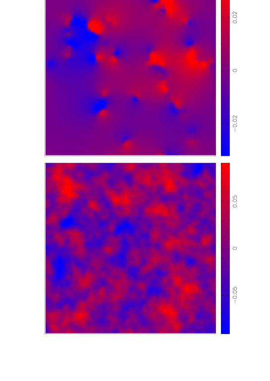
Figure 2: The Kaiser Stebbins effect from cosmic strings (top) if the glow out of the last scattering surface were homogeneous. Adding on the perturbations induced by strings before last scattering leaves what looks like a Gaussian map (bottom).

The formalism we have just outlined acts as comprehensive formalism for encoding non-Gaussianity, which is an advantage over Gaussianity tests. Also, unlike the $n$-point correlation function, it does not contain redundant information. However it lives naturally in Fourier space. This contradicts a well established dogma: non-Gaussianity is obvious in real space, but gets diluted in Fourier space. According to this argument a Fourier mode is the result of the addition of many possibly non-Gaussian temperatures:

$$a({\bf k})={\int{d{\bf k}\over 2\pi}\frac{\Delta T({\bf x})}{T}e^{-i{\bf k}\cdot{\bf x}}}$$ (4)

The central limit theorem then tells us that even if the $\frac{\Delta T({\bf x})}{T}$ are very non-Gaussian the $a({\bf k})$ will be approximately Gaussian. As an example we may consider the Kaiser-Stebbins effect from cosmic strings (see Fig. 2, top figure). Distinctive stringy discontinuities may be recognised in the top map. The Fourier transform of such a map would be a bit of a mess, a mess that is not particularly non-Gaussian.

We will counter this argument using precisely the example of cosmic string maps. These have been oversimplified in the past, in a way that over rates their non-Gaussinity. A more realistic examination of stringy skies does not comply with the cubist microwave sky often attributed to cosmic strings. To begin with realistic cosmic strings are rather contorted objects. As the top figure in Fig. 2 shows one does see jumps on stringy skies but these have a rather limited coherence length.

More important than this is the recognition that even the top picture in Fig. 2 is a simplification. It assumes that the glow of photons coming out of the last scattering surface is perfectly homogeneous. However one must remember that there were strings before last scattering. These also caused fluctuations in the cosmic radiation. After last scattering radiation is made up of free photons that fly past the moving strings and “take a picture” of the string network. Before last scattering the photons behaved more like a fluid, which was slashed by the strings, but was also subject to its own pressure. A complete mess of waves may be expected, rather than a neat picture of the string network. Indeed the only available calculation of string perturbations before last scattering shows rather Gaussian looking fluctuations $\!{}^{{\bf?}}$.

Figure 3: Schematic representation of the power spectrum of the Gaussian fluctuations induced by cosmic strings before last scattering and the non-Gaussian fluctuations induced after last scattering by the Kaiser-Stebbins effect. We also indicate the scale of the inter-string separation at last scattering, which is $\theta\approx 20^{\prime}$ corresponding to $\ell\approx 60^{\circ}/\theta\approx 200$.

One may plot the power spectrum of the fluctuations induced by cosmic strings schematically as in Fig. 3. The $C_{\ell}$ may be seen as the result of two contributing components. One corresponds to fluctuations induced by strings after last scattering, which gives the beautiful Kaiser-Stebbins effect one usually pictures. The other corresponds to the fluctuations induced before last scattering, which should be roughly Gaussian. The non-Gaussian component dominates on large scales, presenting a slightly tilted spectrum $\!{}^{{\bf?}}$, then falls off as a power law $\!{}^{{\bf?}}$. The Gaussian component is negligible at large scales (white noise, rather than quasi-scale invariant), then rises into a single Doppler peak of height as yet unknown, but roughly placed at $\ell\approx 400-600$ $\!{}^{{\bf?}}$. It then falls off exponentially, due to Silk damping .

Figure 4: The Fourier space structure of realistic string skies.

If the Gaussian component were not there all one would need would be an experiment with a resolution better than the inter-string separation at last scattering, and the Kaiser-Stebbins effect would emerge in all its glory. However at the inter-string separation scale the power of the fluctuations is dominated by the Gaussian component. Still not all is lost. Because the Gaussian component falls off as an exponential, whereas the non-Gaussian component falls off like a power law, at very high $\ell$ the fluctuations should be dominated by the non-Gaussian component again. All in all the Fourier space image of a stringy sky may be divided into mainly Gaussian and mainly non-Gaussian bands, as depicted in Fig. 4. It looks as if realistic string maps lead to the conclusion that one needs much higher resolution to detect strings than previously thought, and that their detection will probably be clearer in the Fourier domain.

We are now in position to reverse the central limit theorem argument so often used against non-Gaussianity analysis in the Fourier domain. The real space temperature is now seen as the sum of many Fourier space components, some of which are strongly non-Gaussian, and some others nearly Gaussian:

$$\frac{\Delta T({\bf x})}{T}={\int{d{\bf k}\over 2\pi}a({\bf k})e^{i{\bf k}\cdot{\bf x}}}$$ (5)

The central limit theorem can now, even more than before, predict that the real space imagine will be nearly Gaussian. The bottom figure in Fig. 2 shows that indeed the realistic Kaiser-Stebbins effect does not lead to any structures which any conceivable Human could visually recognise.

Clearly we have a situation where the Gaussian and non-Gaussian components are naturally separated in Fourier space. The non-Gaussian signal in Fourier space will never be a visual signal. However it should be now clear that if I find an algebraic way to detect stringiness in Fourier space, this method will be robust against the addition of Gaussian signal or even Gaussian noise, as long as a non-Gaussian band in Fourier space survives these additions.

Non-Gaussian spectra provide such an algebraic tool. They define shape on a given scale. They should therefore allow the detection of stringy shapes on the outer non-Gaussian band where the stringy Kaiser-Stebbins effect dominates the signal.

4 Non-Gaussian spectra

A more mathematical definition of non-Gaussian spectra will now be given. Consider a ring of the Fourier space where $N_{k}$ independent complex modes $a({\bf k}_{i})=\Re[a({\bf k}_{i})]+i\Im[a({\bf k}_{i})]$ live. In Gaussian theories these are distributed as

$$F(\Re[a({\bf k}_{i})],\Im[a({\bf k}_{i})])={1\over(2\pi\sigma^{2})^{N_{k}/2}}\times$$

$$\exp{-\left({1\over 2\sigma_{k}^{2}}\sum_{i=1}^{m_{k}}(\Re^{2}[a({\bf k}_{i})]+\Im^{2}[a({\bf k}_{i})])\right)}$$ (6)

where $m_{k}=N_{k}/2$. First separate the $N_{k}$ complex modes into $m_{k}$ moduli $\rho_{i}$ and $m_{k}$ phases $\phi_{i}$

$$\Re[a({\bf k}_{i})] = \rho_{i}\cos{\phi_{i}}$$

$$\Im[a({\bf k}_{i})] = \rho_{i}\sin{\phi_{i}}$$ (7)

The Jacobian of this transformation is

$$\left|{\partial(\Re[a({\bf k}_{i})],\Im[a({\bf k}_{i})])\over\partial(\rho_{i},\phi_{i})}\right|=\prod_{i=1}^{m_{k}}\rho_{i}$$ (8)

The $\{\rho_{i}\}$ may be seen as Cartesian coordinates which we transform into polar coordinates. These consist of a radius $r$ plus $m_{k}-1$ angles $\tilde{\theta}_{i}$ given by

$$\rho_{i}=r\cos{\tilde{\theta}_{i}}\prod_{j=0}^{i-1}\sin{\tilde{\theta}_{j}}$$ (9)

with $\sin{\tilde{\theta}_{0}}=\cos{\tilde{\theta}_{m_{k}}}=1$. In terms of these variables the radius is related to the angular power spectrum by $C(k)=r^{2}/(2m_{k})$. In general the first $m_{k}-2$ angles $\tilde{\theta}_{i}$ vary between $0$ and $\pi$ and the last angle varies between 0 and $2\pi$. However because all $\rho_{i}$ are positive all angles are in $(0,\pi/2)$. The Jacobian of this transformation is

$$\left|{\partial(\rho_{1},\cdots,\rho_{m_{k}})\over\partial(r,\tilde{\theta}_{1},\cdots,\tilde{\theta}_{m_{k}-1}}\right|=r^{m_{k}-1}\prod_{i=2}^{m_{k}-1}\sin^{m_{k}-i}{\tilde{\theta}_{i-1}}$$ (10)

Polar coordinates in $m_{k}$ dimensions may be understood as the iteration of the following rule:

$$\rho_{i} = r_{i}\cos{\tilde{\theta}_{i}}$$

$$r_{i-1} = r_{i}\sin{\tilde{\theta}_{i}}$$ (11)

in which $r_{i}$ is the radius of the shade $m_{k}-i+1$ dimensional sphere obtained by keeping fixed all $\rho_{j}$ for $j=1,\cdots,i-1$:

$$r_{i}={\sqrt{\rho_{i}^{2}+\rho_{i+1}^{2}+\cdots+\rho_{m_{k}}^{2}}}$$ (12)

One may easily see that this is how 3D polars work, and also that the transform (9) follows this rule. Hence one may invert the transform (9) with

$$\tilde{\theta}_{i}=\arccos{\rho_{i}\over{\sqrt{\rho_{i}^{2}+\rho_{i+1}^{2}+\cdots+\rho_{m_{k}}^{2}}}}$$ (13)

for $i=1,\cdots,m_{k}-1$.

The Jacobian of the transformation from $(\Re[a({\bf k}_{i})],\Im[a({\bf k}_{i})])$ to $\{r,\tilde{\theta}_{i},\phi_{i}\}$ is just the product of (8) and (10). Hence for a Gaussian theory one has the distribution

$$F(r,\tilde{\theta}_{i},\phi_{i})={{r^{N_{k}-1}\exp{-\left(r^{2}\over 2\sigma_{k}^{2}\right)}}\over(2\pi\sigma^{2})^{N_{k}/2}}\prod_{i=1}^{m_{k}-1}\cos{\tilde{\theta}_{i}}(\sin{\tilde{\theta}_{i}})^{N_{k}-2i-1}$$ (14)

In order to define $\tilde{\theta}_{i}$ variables which are uniformly distributed in Gaussian theories one may finally perform the transformation on each $\tilde{\theta}_{i}$:

$${\theta_{i}}=\sin^{N_{k}-2i}(\tilde{\theta}_{i})$$ (15)

so that for Gaussian theories one has:

$$F(r,{\theta}_{i},\phi_{i})={r^{N_{k}-1}e^{-r^{2}/(2\sigma_{k}^{2})}\over 2^{m_{k}-1}(m_{k}-1)!}\times 1\times\prod_{i=1}^{m_{k}}{1\over 2\pi}$$ (16)

The factorization chosen shows that all new variables are independent random variables for Gaussian theories. $r^{2}$ has a $\chi^{2}_{N_{k}}$ distribution, the “shape” variables $\theta_{i}$ are uniformly distributed in $(0,1)$, and the phases $\phi_{i}$ are uniformly distributed in $(0,2\pi)$.

The variables $\theta_{i}$ define a non-Gaussian shape spectrum, the ring spectrum. They may be computed from ring moduli $\rho_{i}$ simply by

$${\theta}_{i}={\left(\rho_{i+1}^{2}+\cdots+\rho_{m_{k}}^{2}\over\rho_{i}^{2}\cdots+\rho_{m_{k}}^{2}\right)}^{m_{k}-i}$$ (17)

They describe how shapeful the perturbations are. If the perturbations are stringy then the maximal moduli will be much larger than the minimal moduli. If the perturbations are circular, then all moduli will be roughly the same. This favours some combinations of angles, which are otherwise uniformly distributed. In general any shapeful picture defines a line on the ring spectrum $\theta_{i}$. A non-Gaussian theory ought to define a set of probable smooth ring spectra peaking along a ridge of typical shapes.

We can now construct an invariant for each adjacent pair of rings, solely out of the moduli. If we order the $\rho_{i}$ for each ring, we can identify the maximum moduli. Each of these moduli will have a specific direction in Fourier space; let ${\bf k}_{max}$ and ${\bf k}^{{}^{\prime}}_{max}$ be the directions where the maximal moduli are achieved. The angle

$$\psi(k,k^{\prime})={1\over\pi}{\rm ang}({\bf k}_{max},{\bf k}^{{}^{\prime}}_{max})$$ (18)

will then produce an inter-ring correlator for the moduli, the inter-ring spectra. This is uniformly distributed in Gaussian theories in $(-1,1)$. It gives us information on how connected the distribution of power is between the different scales.

We have therefore defined a transformation from the original modes into a set of variables $\{r,\theta,\phi,\psi\}$. The non-Gaussian spectra thus defined have a particularly simple distribution for Gaussian theories. The fact that this distribution does not have a peak shows clearly that we cannot use non-Gaussian spectra to find out anything about the parameters of a Gaussian theory (eg. cosmological parameters in inflation). We shall call perturbations for which the phases are not uniformly distributed localized perturbations. This is because if perturbations are made up of lumps statistically distributed but with well defined positions then the phases will appear highly correlated. We shall call perturbations for which the ring spectra are not uniformly distributed shapeful perturbations. We will identify later the combinations of angles which measure stringy or spherical shape of the perturbations. This distinction is interesting as it is in principle possible for fluctuations to be localized but shapeless, or more surprisingly, to be shapeful but not localized. Finally we shall call perturbations for which the inter-ring spectra are not uniformly distributed, connected perturbations. This turns out to be one of the key features of stringy perturbations. These three definitions allow us to consider structure in various layers. White noise is the most structureless type of perturbation. Gaussian fluctuations allow for modulation, that is a non trivial power spectrum $C(k)$, but their structure stops there. Shape, localization, and connectedness constitute the three next levels of structure one might add on. Standard visual structure is contained within these definitions, but they allow for more abstract levels of structure.

5 The meaning of non-Gaussian spectra

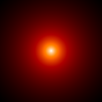
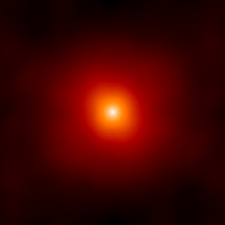
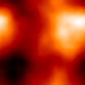
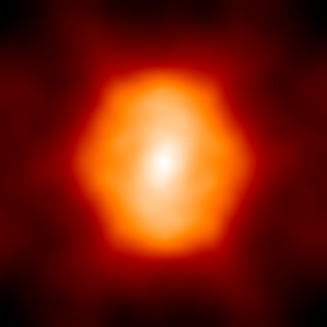
Figure 5: A spherical hot spot which has been deconstructed at different levels. On the top left hand panel we have the pure non-Gaussian signal. The angles $\theta_{i}$ have been redrawn uniformly on the top right picture. On the bottom left the phases $\phi_{i}$ were redrawn unformly. On the bottom right we applied an independent unformly distributed rotation on all rings in Fourier space. From top to bottom and left to right, a plain regular sphere, a shapeless sphere, a delocalized sphere, and a disconnected sphere.

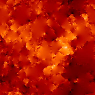
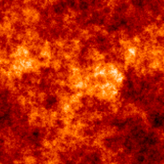
Figure 6: The Kaiser-Stebbins effect (top left) and its various stages of deconstruction. The angles $\theta_{i}$ have been redrawn uniformly on the top right picture. On the bottom left the phases $\phi_{i}$ were redrawn unformly. On the bottom right we applied an independent unformly distributed rotation on all rings in Fourier space. Respectively we have strings, shapeless strings, unlocalized strings and disconnected strings.

The decomposition $\{C(k),{\theta},\phi,\psi\}$ has an immediate physical interpretation. The angles $\theta$ reflect the angular distribution of power, and therefore reflect shape. The phases $\phi$ transform under translations and so contain the information on position and localization of the structures in the field. The angles $\psi$ correlate different scales, and therefore tell us how connected the structures are. For a Gaussian random field the variables $\{{\theta},\phi,\psi\}$ are all uniformly distributed reflecting complete lack of structure besides the power spectrum. In terms of the various levels of structure considered we can then characterize Gaussian fluctuations as shapeless, delocalized and disconnected. By comparison with a Gaussian we may then define structure at different levels. We will say that fluctuations for which ${\theta}$ are not uniformly distributed are shapeful. If the $\phi$ are not uniformly distributed we shall say the fluctuations are localized. If the $\psi$ are not uniformly distributed the fluctuations are connected. Although visual structure has room within these definitions, they are considerably more abstract and general. We may consider highly non visual types of structure such as shapeful but delocalized fluctuations or disconnected localized stringy fluctuations. In this sense we regard our formalism as a robust definition of structure, which goes beyond what is visually recognazible and so is tied down to our particular and narrow path of natural selection. We may imagine an alien civilization with Fourier space eyes (say interferometric eyes $\!{}^{{\bf?}}$), and a brain trained to recognize Fourier space structure at many different levels, structure that would seem totally non obvious to our human eyes.

To illustrate the limitations of human vision we shall now destroy highly structured maps level by level, that is Gaussianize only one of the variable types $\{{\theta},\phi,\psi\}$. Initially there will be structure at every level, shape, position, and connectedness. We will remove structure gradually, a fact not disasterous for the alien civilization referred above, but which will illustrate the limitations of the human visual method for recognizing non-Gaussianity. In Figure 5 we play this game with a sphere. We depict a spherical hot spot in real space, then a shapeless sphere, a delocalized sphere, and a disconnected sphere. For the case of a sphere we find that what we recognize as shape is mostly localization. A shapeless sphere keeps its recognizable features. On the other hand a delocalized sphere loses it characteristic features. Indeed the idea of a shapeful but non-localized object sounds somewhat surreal for all we can visually conceptualize. Nevertheless our formalism will acuse the strong but not obvious non-Gaussianity exhibited by a delocalized sphere.

In Figure 6 we repeat the same exercise for a map displaying the Kaiser-Stebbins effect from cosmic strings. Shapeless strings, delocalized strings, and disconnected strings are shown. Considerable disarray is introduced in every case, but one may say that disconnected strings as well as delocalized strings are perhaps the most messy of them. This is consistent with the strong signal in $\psi$ we have found for the case of the realistic Kaiser Stebbins effect. On the other hand the fact that line-like discontinuities are present even for shapeless strings shows how much more structure there is in the map on top of the structure which we can recognize. This is important since the beautiful patchwork is very fragile to the hard realities of noise and supperposed Gaussian signal. In the real world, it turns out, the non-visual feature which is the connectedness of strings happens to survive much better than the patchwork (which reflects mostly localization).

6 Non-Gaussian spectra and cosmic string detection

As shown in Sec.3 the existence of a Gaussian background in string scenarios implies the need for higher resolution than thought before in order to detect cosmic string non-Gaussianity. Interferometer experiments are therefore favoured. For such high resolution interferometers can only look into small fields. We therefore concentrate on a field of some $20^{\prime}$ across. The Kaiser-Stebbins effect before and after the addition of the Gaussian signal would then look like Fig. 7.

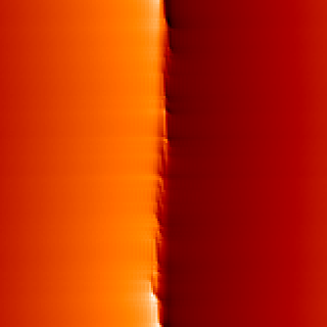
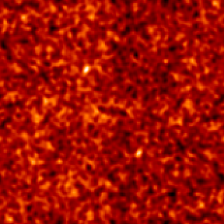
Figure 7: A field of the order of $20^{\prime}$ across showing the Kaiser-Stebbins effect from a cosmic string before and after the Gaussian signal is added.

Clearly the string is no longer visible. What is more, we have checked that the traditional non-Gaussianity tests fail to detect the hidden small scale non-Gaussianity in the right picture in Fig. 7. We have checked this statement with: pixel histograms, skewness and kurtosis, density of peaks, topological tests, the 3-point correlation function, and other traditional tests. As an example we show in Fig. 8 the failure of the Euler characteristic test to detect the realistic Kaiser-Stebbins effect.

Figure 8: The mean Euler characteristic, $\Gamma$ as a function of threshold for a string map with Gaussian noise (solid line) and for a pure Gaussian map with the same power spectrum (the shaded region is the 1 $\sigma$ region around the Gaussian mean, estimated from a 100 realizations).

However we found that non-Gaussian spectra may still detect the hidden string after Gaussian signal has been added. Let us first look at shape spectra (Fig. 9). For rings at low $k$ these are very Gaussian. However, as we go out into high $k$ rings, something peculiar starts to happen. The straight string spectrum is of course never visible. However a clear ridge in the distribution of shapes emerges. This corresponds to the wiggly string shape. There is naturally cosmic/sample variance in the shape spectrum. This is because not all wiggly strings have the same wiggles. Therefore, as in the case of $C_{\ell}$ spectra, one must complement the average spectrum with error bars. Still the concept of shape spectrum makes sense, because shapes are not uniformly distributed, but rather have a peaked distribution.

Figure 9: The ring spectrum at high $k$ inferred from 100 realizations. The shaded region represents a probability larger than $1\over e$ for the the values of $\theta_{i}$ to occur (this generalises the concept of 1 sigma error bar for non-Gaussian distributions.

More impressive still is the inter-ring spectrum, shown in Fig. 10. If an object is exactly stringy then it concentrates the power in Fourier space along one direction. More importantly, this direction is the same for adjacent rings. Then, for wiggly strings, one may expect that the direction where the maximum modulus is achieved is highly correlated from ring to ring. As we see in Fig. 10, as we go up in $k$ the angle $\psi$ between maximal directions is at first uniformly distributed. Gradually, as the string signal starts to dominate, the $\psi$ distribution becomes highly peaked around $\psi=0$. This is a very impressive signal, with a very small error bar. We put most of our hopes of detection on this signal.

Figure 10: The inter-ring spectrum $\psi$. The shaded region represents a probability larger than $1\over e$ for the the values of $\psi_{i}$ to occur.

7 Prospects for the future

The statistics presented here should be comprehensive in their detection of non-Gaussianity, but naturally we are concentrating on finding characteristic signatures for string networks in this framework.

7.1 Simulating the sky

We plan to test our statistics on actual observations. But before using real data, we need to test the method on simulations. We are currently working on simulated brownian strings. These are useful in testing our intuition about the statistics but of course are not the most realistic examples of strings. The most accurate string maps are generated by evolving a string network from its initial conditions up to the present. We will do this by means of the integer string code described in $\!{}^{{\bf?}}$. We hope to generate 10000 maps in this way.

Once we have a string map, the photon temperature map is calculated using Laplace’s equation $\!{}^{{\bf?}}$

$${\nabla}^{2}\frac{\Delta T}{T}=-8\pi G{\vec{\nabla}}\cdot{\vec{U}}$$ (19)

where all operations here are on the plane orthogonal to some direction vector ${\vec{n}}$. If ${\vec{n}}$ is chosen to be in the $z$ direction then we have

$$U_{i}=-\int_{-\infty}^{+\infty}[\Theta_{0i}(t,X_{\gamma}(t))-\Theta_{i3}(t,X_{\gamma}(t))]dt$$ (20)

where $\Theta_{\mu\nu}$ is the stress-energy tensor for a string and $i=1,2$. Laplace’s equation is most easily solved in Fourier space so we are like an interferometer experiment, which observes directly in Fourier space.

We will assume the fluctuations on the last scattering surface to be Gaussian, so all we need to specify is the power spectrum. As the height of the peak in the spectrum is unknown for defect models and its position is uncertain we need to fit parameters to the $C_{\ell}$.

7.2 Simulating the experiment

First we have to take into account effects of limited sky coverage and resolution. This is done for an interforemeter by modelling the primary beam of the antennae with a window function $W(\bf{x})$ in real space and the synthesized beam by a function $B(\bf{x})$. The Fourier transform of $B(\bf{x})$, $\tilde{B}(\bf{k})$, is 1 where the Fourier domain is sampled and 0 otherwise so it is effectively a window in Fourier space. Therefore the limit of resolution in real space places an upper limit on the values of $k$ we can look at. Large values of $k$ are precisely what we want to look at, so we hope for a high resolution experiment. The Fourier transform of $W(\bf{x})$, $\tilde{W}(\bf{k})$, corresponds to a limit in the resolution in Fourier space since $W(\bf{x})$ cuts off large scales in real space. This introduces correlations in the $a(\bf{k})$, so we must be careful in deciding how to sample Fourier space.

Foreground emission can be split into two main components: smooth emission from dust, synchrotron and free-free emission and point sources. Smooth emission gives approximately constant errors for all $k$ so it can be modelled as Gaussian noise (see below). Spherical point sources have $\rho_{i}={\rm constant}$ in each ring, so they should not interfere with the ring spectra of strings.

Finally we need to add noise to our sky map. This is assumed to be Gaussian. It adds an extra term to the covariance matrix of the Fourier modes $a(\bf k)$ which may be written as $\!{}^{{\bf?}}$

$${\langle a^{N}({\bf k}_{i}),a^{N}({\bf k}_{j})\rangle}=\delta_{ij}\frac{\omega^{-1}n_{\rm f}\Omega^{3}}{(2\pi)^{2}}$$ (21)

with $\omega^{-1}=\frac{As^{2}}{t_{\rm tot}}$, where $A$ is the area of Fourier space covered, $s^{2}$ is the sensitivity of the detector, $t_{\rm tot}$ is the total observing time, $n_{\rm f}$ is the number of fields observed and $\Omega$ is the area of each field. We will experiment with the various parameters to find the best observing strategy.

7.3 The statistics

Once we have our maps of stringy skies we can test the statistics on them so we will be in a position to decide what the best observing strategies are (ie how long should be spent in each field, how many fields should be observed etc).

Other possibilities for statistics to investigate include:

• Quantities made up of the phases of the $a(\bf k)$ (in the same way that the shape spectra are made up of the moduli). The phases contain all the information about position in real space and so are complementary to the moduli.

• Looking at the two point function around a ring in Fourier space.

• Taking another Fourier transform in angle around a ring in Fourier space. This and the two point function are alternative ways of looking at the distribution of power in rings.

Eventually we hope to test our statistics on data from the VLA and BIMA experiments. These are interferometer experiment with a field of a few arcminutes but very high resolution and sensitivity.

References

References

- [1] P.Ferreira and J.Magueijo, “Non-Gaussian spectra”, to be published in PRD.
- [2] N.Turok, Sub-degree Scale Microwave Anisotropies from Cosmic Defects, astro-ph/9606087.
- [3] Allen et al, astro-ph/9609038.
- [4] M.Hindmarsh, Astrophys.J. 431 (1994) 534.
- [5] A.Albrecht et al, Phys.Rev.Lett 76 1413-1416 (1996), Magueijo et al ibid 2617 (1996), Magueijo et al Phys.Rev D 54 3727 (1996).
- [6] R.Battye, astro-ph/9610197.
- [7] After all we have Fourier space ears. We thank Dr.K.Baskerville for this pertinent remark.
- [8] J.Borrill, PRD 50 2469 (1994)
- [9] M.Hobson,J.Magueijo, astro-ph/9603064, to be published in MNRAS.
- [10] Coulson et al, Nature 368 27-31 (1994).