Forecasting Cosmic Parameter Errors from Microwave Background Anisotropy Experiments

Abstract

Accurate measurements of the cosmic microwave background (CMB) anisotropies with an angular resolution of a few arcminutes can be used to determine fundamental cosmological parameters such as the densities of baryons, cold and hot dark matter, and certain combinations of the cosmological constant and the curvature of the Universe to percent-level precision. Assuming the true theory is a variant of inflationary cold dark matter cosmologies, we calculate the accuracy with which cosmological parameters can be determined by the next generation of CMB satellites, MAP and Planck. We pay special attention to: (a) the accuracy of the computed derivatives of the CMB power spectrum ${\rm C}_{\ell}$; (b) the number and choices of parameters; (c) the inclusion of prior knowledge of the values of various parameters.

1 Introduction

The detection of primordial anisotropies in the microwave background radiation by the COBE satellite (Smoot et al. 1992) has had an enormous impact on cosmology (see White, Scott and Silk 1994 and Bond 1996 for reviews). However, the relatively poor angular resolution of COBE/DMR ($\theta_{fwhm}\approx 7^{\circ}$) limits the amount of information that can be extracted from the CMB. From the 4 year COBE maps (Bennett et al. 1996a), the overall amplitude of the CMB power spectrum for a given spectral shape has been determined to an accuracy of $7\%$ and a power law index characterizing the shape to $\pm 0.24$ (Bond 1996). Constraints on other parameters such as the spatial curvature and the cosmological constant $\Lambda$ are weak.

It has long been known (Sunyaev and Zeldovich 1970) that at angular resolutions smaller than $\sim 1^{\circ}\Omega_{0}^{1/2}$ (the angle subtended by the Hubble radius at the time of recombination) the CMB power spectrum will depend on e.g., the sound speed of the baryon-photon fluid, and hence on a number of fundamental cosmological parameters, such as the densities of baryons, cold and hot dark matter, and the spatial curvature of the Universe. In adiabatic models, the acoustic motions of the matter radiation fluid lead to a characteristic series of ‘Doppler peaks’ in the CMB power spectrum which have been investigated in considerable detail numerically and semi-analytically (e.g., Bond 1996, Hu et al. 1997). Similar behaviour is expected qualitatively in defect (isocurvature) theories, though the pattern of Doppler peaks is expected to be less distinct and has not yet been calculated to high precision (e.g., Turok 1996). We therefore restrict the discussion in this paper to purely adiabatic perturbations obeying Gaussian statistics, as expected in most inflationary models of the early universe (e.g., Linde 1990). The anisotropies in such models can be computed to high accuracy which, as we will show in Section 2, is essential for estimating the precision with which cosmological parameters can be determined from the CMB.

Intermediate angle experiments have detected temperature anisotropies which are consistent with a primordial origin and in rough agreement with adiabatic theory predictions. However, the accuracy and robustness of the results does not yet allow strong conclusions to be drawn, even when experimental results are combined together (e.g., Bond 1996, Bond & Jaffe 1997, Lineweaver et al. 1997, Rocha & Hancock 1997). An experiment with an angular resolution of $\theta_{fwhm}\sim 5^{\prime}$ can yield useful information about the CMB spectrum ${\rm C}_{\ell}$ up to multipoles beyond a Gaussian filtering scale $\ell_{s}=\sqrt{8\ln 2}\theta_{fwhm}^{-1}\sim 2000$. If the sky coverage is complete, each multipole is statistically independent. However, it is clear from visual inspection (e.g. Figure 1) that a typical inflationary ${\rm C}_{\ell}$ curve is smooth and can be specified accurately by many fewer than $2000$ parameters. It is therefore not obvious a priori to what extent the typically 10-15 parameters specifying an inflationary model can be disentangled by a particular set of measurements. Evidently, a detailed calculation is necessary as has been performed in an important paper by Jungman et al. (1996). However, as described in the next section, an accurate assessment of the degeneracies between cosmological parameters imposed by high resolution CMB experiments requires a precise numerical calculation, rather than the semi-analytic approach adopted by Jungman et al.

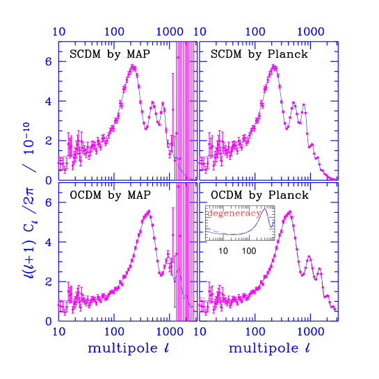
Figure 1: Temperature power spectra for a standard CDM (SCDM) model with ${\rm h}=0.5$, $\Omega_{m}=1$ and $\Omega_{\Lambda}=0$ and an open CDM (OCDM) model with ${\rm h}=0.6$ , $\Omega_{m}=0.33$ and $\Omega_{\Lambda}=0$. The points show a quadratic power spectrum estimation of ${\rm C}_{\ell}$ (in bands of width 5% in $\ell$), along with the one sigma error, from simulated CMB skies observed by the MAP and Planck satellites described in Section 3 and Table 1. The errors in the left panels use the MAP⁺ parameters for the three highest frequency channels and two years of observing, while those in the right panels use the four lowest frequency Planck HFI channels. Planck can follow the theoretical curves quite precisely far down the damping tail for both models. In the bottom right panel, a ${\rm C}_{\ell}$ curve with $\Omega_{m}=0.15$, $\Omega_{\Lambda}=0.44$ and ${\rm h}=0.9$ almost degenerate with the OCDM model is superposed. The inset, showing these two and also a $\Omega_{m}=0.10$, $\Omega_{\Lambda}=0.58$ and ${\rm h}=1.1$ model, demonstrate that the angle-distance degeneracy relation (see text) used to define these models is almost exact; these models can be distinguished only at low multipoles no matter how precise the CMB experiment.

2 Parameter estimation with priors

2.1 The covariance matrix

Errors on a set of cosmological parameters ${\bf s}=\{s_{i}\},i=1,\ldots,n$ are estimated using Bayes theorem, which updates the prior probability $P({\bf s}|{\rm prior})$ for the parameters with a likelihood function ${\cal L}({\bf s})$: $P({\bf s})\propto{\cal L}({\bf s})P({\bf s}|{\rm prior})$. (Although a uniform prior seems to be the least prejudicial, there are certain non-debatable restrictions and plausible constraints which are reasonable to include as prior information, as discussed in Section 2.5.) If the errors $\delta{\bf s}$ $\equiv{\bf s}-{\bf s_{\circ}}$ about the mean ${\bf s_{\circ}}=\langle{\bf s}\rangle$ are small, then an expansion of $\ln{\cal L}$ to quadratic order about the maximum gives:

$${\cal L} \approx {\cal L}_{m}\exp\left[-{\textstyle{1\over 2}}\sum_{ij}{F}_{ij}\delta s_{i}\delta s_{j}\right]\,,$$

$${F}_{ij} = \sum_{\ell}(\Delta{\rm C}_{\ell})^{-2}{\partial{\rm C}_{\ell}\over\partial s_{i}}{\partial{\rm C}_{\ell}\over\partial s_{j}}\,,$$ (1)

$$(\Delta{\rm C}_{\ell})^{2} \approx {2\over(2\ell+1)f_{sky}}\,\left({\rm C}_{\ell}+\overline{w}^{-1}\overline{{\cal B}}_{\ell}^{-2}\right)^{2}\,,$$ (2)

$$\overline{w} \equiv \sum_{c}w_{c},\quad\overline{{\cal B}}_{\ell}^{2}\equiv\sum_{c}{\cal B}^{2}_{c\ell}w_{c}/\overline{w},$$ (3)

$$w_{c} \equiv (\sigma_{c,pix}\theta_{c,pix})^{-2},\quad{\cal B}^{2}_{c\ell}\approx e^{-\ell(\ell+1)/\ell_{s}^{2}},$$

adopting a Gaussian approximation for the beam function ${\cal B}_{c\ell}$. In this approximation, with a uniform prior the covariance matrix ${\bf M}\equiv\langle\delta{\bf s}\delta{\bf s}^{\dagger}\rangle$ is the inverse of the Fisher information matrix ${\bf F}$ (e.g., Tegmark et al. 1997), the 1-sigma error on $s_{i}$ is $\sigma_{i}=M_{ii}^{1/2}$, and the correlation coefficient between parameters $i$ and $j$ is $r_{ij}=M_{ij}/(\sigma_{i}\sigma_{j})$. Equation (2) gives the standard error $\Delta{\rm C}_{\ell}$ on the estimate of ${\rm C}_{\ell}$ for an experiment with $N$ frequency channels $c$, angular resolution $\theta_{c,fwhm}$, and sensitivity $\sigma_{c,pix}$ per resolution element ($\theta_{c,fwhm}\times\theta_{c,fwhm}$ pixel), which samples a fraction $f_{\rm sky}$ of the sky.

A key simplifying assumption in deriving equation (2) is that the noise is homogeneous and isotropic. Provided that the sampling varies slowly, accurate error estimates can be obtained using the average weight for the experiment. Equation (2) is exact if $f_{sky}=1$ (e.g., Knox 1995) and is approximately correct at multipoles $\ell\mathrel{\hbox to0.0pt{\lower 3.0pt\hbox{$\mathchar 536\relax$}\hss}\raise 2.0pt\hbox{$\mathchar 318\relax$}}\ell_{cut}$ corresponding to angular scales small compared to the dimensions $2\pi/\ell_{cut}$ of an incomplete sky map.

The accuracy of cosmological parameter estimation via the covariance matrix approach depends on: (1) the validity of the Gaussian approximation to the likelihood function; (2) the number and choice of the parameters ${\bf s}$ defining the theoretical model; (3) the parameters ${\bf s_{\circ}}$ of the target model; (4) the numerical accuracy of the derivatives of ${\rm C}_{\ell}$; (5) the inclusion of prior constraints on the parameters ${\bf s}$; (6) systematic errors in estimates of ${\rm C}_{\ell}$ caused by Galactic and extragalactic foregrounds. For high resolution experiments which tightly constrain many of the cosmological parameters, a Gaussian approximation about the maximum likelihood should be quite good (Knox 1995, Spergel private communication), although positivity and other constraints can truncate general excursions in the likelihood space. We ignore systematic errors caused by foreground subtraction, since over much of the sky these are very likely to be much smaller than the variance of equation (2) (see e.g. Tegmark and Efstathiou 1996 for a discussion of foreground removal from CMB maps). Here we consider the remaining four points.

2.2 Choice of variables

Parameters describing the theoretical angular power spectra include those for initial conditions and those characterizing the transport of radiation through photon decoupling to the present. If we were to allow all possible variations, the count of parameters could easily exceed $20$; in our analysis, we use $\mathrel{\hbox to0.0pt{\lower 3.0pt\hbox{$-$}\hss}\raise 2.0pt\hbox{$\mathchar 316\relax$}}11$ variables. We characterize the initial fluctuation spectra by an amplitude and a spectral index (tilt) for the scalar and tensor components, ${\cal P}_{\Phi}^{1/2}(k_{n})$ and $n_{s}$, ${\cal P}_{GW}^{1/2}(k_{n})$ and $n_{t}$. The primordial amplitude parameters for the gravitational potential fluctuations, ${\cal P}_{\Phi}^{1/2}(k_{n})$, and the gravity wave fluctuations, ${\cal P}_{GW}^{1/2}(k_{n})$, are chosen here to be normalized at a wavenumber corresponding to the horizon scale. The fluctuations arising from inflation could be much more complicated, requiring, for example, the parameterization of variations of the spectral indices with wavenumber $k$, inclusion of isocurvature as well as adiabatic components in the scalar perturbations, and possibly of non-Gaussian features.

At the time of decoupling, the key parameters determining the temperature power spectrum are the densities of various types of matter, the expansion rate, the sound speed, and the damping rate; all of these depend only on the density parameters $\omega_{j}\equiv\Omega_{j}{\rm h}^{2}$, where $j=b,cdm,hdm,\gamma,er\nu$ refers to baryons, cold dark matter, hot dark matter, and the various relativistic particles present then, such as photons and relativistic neutrinos. The Hubble parameter at that time only depends upon $\omega_{m}=\omega_{b}+\omega_{cdm}+\omega_{hdm}$ (if the massive neutrinos were nonrelativistic then) and $\omega_{er}=\omega_{\gamma}+\omega_{er\nu}$.

The transport to an angular structure of scale $\ell^{-1}$ now from the post-decoupling spatial pattern of temperature fluctuations of comoving scale $k^{-1}$ depends on the cosmological angle-distance relation, $\ell\sim k{\cal R}$, where

$${\omega_{m}^{1/2}{\cal R}\over 3000{\rm~{}Mpc}} = {\omega_{m}^{1/2}\over\omega_{k}^{1/2}}{\rm sinh}\left[\int{\omega_{k}^{1/2}da\over(\omega_{k}a^{2}+\omega_{\Lambda}a^{4}+\omega_{m}a)^{1/2}}\right]$$

for an open universe (e.g., Bond & Efstathiou 1984). Here $\omega_{\Lambda}\equiv\Omega_{\Lambda}{\rm h}^{2}$ parameterizes the energy density associated with a cosmological constant $\Lambda$ ($\Omega_{\Lambda}=\Lambda/(3H_{0}^{2})$) and $\omega_{k}\equiv(1-\Omega_{0}){\rm h}^{2}$ = $(1-\Omega_{m}-\Omega_{\Lambda}){\rm h}^{2}$ parameterizes the energy associated with the mean curvature of the universe. This results in a degeneracy along ${\delta(\omega_{m}^{1/2}{\cal R})}=0$ lines, which leads to a linear relation between $\delta\omega_{k}$ and $\delta\omega_{\Lambda}$ for fixed $\omega_{m}$, with coefficients that depend upon the explicit target model. The angular pattern we observe also depends upon the change of the gravitational metric in time between post-decoupling and the present, which breaks this degeneracy. However, this late-time integrated Sachs-Wolfe effect influences only low multipoles which have a large cosmic variance. Thus, there exists one combination of variables which cannot be determined accurately from CMB observations alone, even with a high precision experiment such as the Planck Surveyor, as the lower right panel of Fig. 1 illustrates.

Some parameters are tightly constrained by measurements other than CMB anisotropies. For example, $\omega_{\gamma}$ depends on the temperature $T_{0}$ of the CMB, $\omega_{er\nu}$ depends as well on the number of massless neutrino types; the ${\rm C}_{\ell}$’s also depend on the helium abundance, parameterized by $Y_{He}$. Rather than allow such parameters complete freedom, we use the prior probabilities to restrict their allowed variations. (Since the experimental errors on $Y_{He}$, $T_{0}$ and $N_{\nu}$ are small , they have a weak effect on other cosmological parameters and hence we include only $Y_{He}$ in our analysis to illustrate the methodology.)

There also could be many parameters needed to characterize the ionization history of the Universe; here we use the Compton optical depth $\tau_{C}$ from the present to the redshift of reheating, assuming full ionization. We therefore analyse a maximum of 11 parameters in this paper: $Y_{He}$, $\tau_{C}$, 4 initial condition parameters and 5 density parameters $\omega_{j}$.

For a given model, the amplitudes of the scalar and tensor power spectra are uniquely related to the observed amplitude of the CMB power spectrum and that of the present day mass fluctuations (characterised, for example, by the rms density fluctuation in spheres of radius $8{\,{\rm h}^{-1}~{}\rm Mpc}$, $\sigma_{8}$). For example, Jungman et al. used the quadrupole ${\rm C}_{2}^{1/2}$ to fix the amplitude of the fluctuation spectrum. We use ${\langle\ell(\ell+1){\rm C}_{\ell}/(2\pi)\rangle}_{B}^{1/2}$, an average over the total band $B$ of multipoles that is accessible to the experiment, since this is most accurately determined. However the normalization parameters $\sigma_{8}$ and ${\cal P}_{\Phi}^{1/2}(k_{n})$ are of sufficient interest that we also show the accuracies with which these can be determined. To characterize the tensor amplitude, we use $r_{ts}\equiv{\rm C}^{(T)}_{2}/{\rm C}^{(S)}_{2}$ instead of ${\cal P}_{GW}^{1/2}(k_{n})$. In inflation models, ${\cal P}_{GW}^{1/2}(k_{n})/{\cal P}_{\Phi}^{1/2}(k_{n})$ is simply related to the tensor tilt, with small corrections dependent upon the scalar and tensor tilts, so one of the four initial fluctuation parameters is a function of the other three, here chosen to be $n_{t}$. $r_{ts}$ also depends upon other cosmological parameters as well as the tilts (e.g., Bond 1996, equation (6.38)).

Any parameter set which defines a coordinate system on the likelihood surface is a viable set. However, parameters for which the Fisher matrix analysis is particularly well suited are those for which the first order expansion ${\rm C}_{\ell}={\rm C}_{\ell}({\bf s_{\circ}})+(\partial{\rm C}_{\ell}({\bf s_{\circ}})/\partial{\bf s})\cdot({\bf s}-{\bf s_{\circ}})$ is more accurate than the sampling variance $\Delta{\rm C}_{\ell}$ for parameters ${\bf s}$ that lie within a few standard deviations from the target set ${\bf s_{\circ}}$. The set of variables that we have adopted gives acceptably high accuracy for the CMB experiments described in Section 3.

2.3 Choice of target models

We analyze three spatially flat ($\Omega_{k}=0$) target models and one with negative curvature. For the canonical flat universe we use a standard CDM model (SCDM) with the following parameters: $n_{s}=1$, $n_{t}=0$, $\Omega_{m}=1.0$, $\Omega_{b}=0.05$, $r_{ts}=0$, $\Omega_{cdm}=0.95$, $\Omega_{hdm}=0$, ${\rm h}=0.5$, $\tau_{C}=0$, $Y_{He}=0.23$; it has $\sigma_{8}=1.2$, normalized to match COBE DMR, but with too many clusters to match the observations. The open model has ${\rm h}=0.6$, $\Omega_{m}=0.33$, $\Omega_{b}=0.035$, $\Omega_{cdm}=0.30$ and $\sigma_{8}=0.44$, the COBE-normalization, which has too few clusters. We also discuss results for two other DMR-normalized spatially flat models that more closely match observations: an HCDM model with 2 species of massive neutrinos, $\Omega_{hdm}=0.2,m_{\nu}=2.4\,{\rm~{}eV}$, ${\rm h}=0.5$ and $\sigma_{8}=0.77$; a $\Lambda$CDM model with $\Omega_{\Lambda}=0.67$, ${\rm h}=0.7$ and $\sigma_{8}=1.1$. (All models have a 13 Gyr cosmological age.)

2.4 Accuracy of the power spectrum derivatives

Computational errors in the derivatives of ${\rm C}_{\ell}$ can lead to large errors in the covariance matrix. We distinguish between two classes of error, one caused by inadequate semi-analytic approximations to the ${\rm C}_{\ell}$ and the second caused by numerical errors in ${\rm C}_{\ell}$ and its derivatives computed from linear Boltzmann transport codes. The ${\rm C}_{\ell}$ accuracy must be $1\%$ or better, especially for high resolution experiments probing multipoles $\ell\mathrel{\hbox to0.0pt{\lower 3.0pt\hbox{$\mathchar 536\relax$}\hss}\raise 2.0pt\hbox{$\mathchar 318\relax$}}1000$ where the expected random errors on each individual multipole become $\mathrel{\hbox to0.0pt{\lower 3.0pt\hbox{$\mathchar 536\relax$}\hss}\raise 2.0pt\hbox{$\mathchar 316\relax$}}3\%$. Errors which are weakly correlated with physical parameters are particularly serious since these can artificially break real near-degeneracies between cosmological parameters and lead to overly optimistic error estimates, sometimes by an order of magnitude or more. Extreme care is therefore required in computing the ${\rm C}_{\ell}$ derivatives. For this work we have used derivatives calculated with two Boltzmann transport codes, an updated version of the multipole code described by Bond and Efstathiou (1987) generalized to low density universes and including tensor components (Bond 1996 and references therein), and the fast path-history code developed recently by Seljak and Zaldarriaga (1996). Generally the ${\rm C}_{\ell}$’s from these codes agree to better than $1\%$. We use intervals of typically $1-5\%$ in the parameters ${\bf s}$ in computing numerical derivatives of ${\rm C}_{\ell}$, i.e. small enough that the derivatives are insensitive to the size of the interval, but large enough that they are unaffected by numerical errors in the ${\rm C}_{\ell}$ coefficients. The primary limitation on the error estimates for Table 2 should be the ${\rm C}_{\ell}$ linearization assumption made in deriving equation 1, although we believe that better than percent level accuracy in ${\rm C}_{\ell}$ is needed to achieve high precision in the nearly degenerate directions of parameter space. The differences between our error estimates and analogous results of Jungman et al. , which are large for some parameters, are caused primarily by their use of semi-analytic approximations to calculate ${\rm C}_{\ell}$ and its derivatives. Zaldarriaga et al. 1997 have undertaken a similar analysis and come to similar conclusions as those presented here. They also showed that polarization information can improve the accuracy of some variables, e.g., $\tau_{C}$, if foregrounds are ignored. Little is known about how the polarization of foregrounds will compromise the relatively weak polarization signal of primary anisotropies, especially at low $\ell$ where much of the improvement comes from. See also related work on forecasting errors by Mageuijo and Hobson (1997).

2.5 Inclusion of prior information on parameters

We have mentioned that a non-uniform $P({\bf s}|{\rm prior})$ is particularly useful for parameters such as $Y_{He}$ and $T_{0}$, where other experiments restrict their values to much higher accuracy than can be achieved from CMB experiments alone. For other parameters, e.g. $\omega_{b}$ and $\omega_{cdm}$, it may be that the distribution derived from a CMB experiment is much narrower than any reasonable prior distribution, in which case we gain little by including prior information. There are also intermediate cases where prior information can help break degeneracies between parameters estimated from the CMB alone. We approximate the prior distribution of parameter values by a Gaussian distribution with covariance matrix ${\bf T}$, so the covariance matrix of parameter values including prior information is given by

$${\bf M}=({\bf F}+{\bf T}^{-1})^{-1}\ {\rm if}\ P({\bf s}|{\rm prior})\propto e^{-{{\textstyle{1\over 2}}\delta{\bf s}^{\dagger}{\bf T}^{-1}\delta{\bf s}}}$$ (4)

(e.g. Knox 1995), where ${\bf F}$ is the Fisher matrix (1). If we are interested in the error bars on $s_{i}$ irrespective of the values of the other variables, we would marginalize over these, with error $\sigma_{i}=M_{ii}^{1/2}$ for the Gaussian case. For most of the entries in Table 2 we use no prior at all (‘no$P$’), except for $Y_{He}$ where indicated. When priors are used, we adopted a diagonal covariance matrix $T_{ij}$ with the following values for $\sqrt{T_{ii}}$: 0.3 on the normalization $\delta{\langle{\cal C}_{\ell}\rangle}_{B}^{1/2}/{\langle{\cal C}_{\ell}\rangle}_{B}^{1/2}$, 0.5 on $n_{s}$, 2 on $r_{ts}$, 0.075 on $\omega_{b}$, 1 on $\omega_{m}$, 1 on $\omega_{\Lambda}$, 1 on $\omega_{k}$, 0.5 on $\omega_{hdm}$, and 1 on $\tau_{C}$. Some variables are restricted for physical reasons to lie within a certain range e.g., $\tau_{C}$ and $r_{ts}$ must be positive. Such constraints can be incorporated into the prior, but at the expense of more complicated expressions after marginalization over these constrained variables. In some cases, imposing physical restrictions can lead to a factor of two or more improvement in the accuracy of the parameter estimates.

Generally the errors in the parameters will be correlated through nondiagonal components of $({\bf F}+{\bf T}^{-1})^{-1}$. Linear combinations of the parameters which are uncorrelated can be found by diagonalizing $({\bf F}+{\bf T}^{-1})$. When the eigenvalues of $({\bf F}+{\bf T}^{-1})$ are rank ordered, from highest to lowest, the variable combinations corresponding to high values will be very accurately determined, while those for the lowest may be very poorly determined, representing the most degenerate directions in parameter space. In Tables 2 and 3 below we list the number of parameter combinations that are determined within a $\pm 0.01$ and $\pm 0.1$ accuracy.

3 Cosmological Parameter Errors from MAP and Planck

3.1 The CMB power spectrum estimated from MAP and Planck

In this section we apply the above machinery to determine the accuracy of cosmological parameter estimation from two satellite experiments: the MAP satellite selected by NASA (Bennett et al. 1996b) and the Planck Surveyor Mission (formerly named COBRAS/SAMBA) selected by ESA (Bersanelli et al. 1996). These satellites offer examples of the best that is likely to be achieved in the next decade. Ground based and balloon borne experiments will certainly continue to provide improved constraints on cosmological parameters over this timescale, and so we also analyze a sample long duration balloon experiment (LDB).

The specifications adopted for MAP and Planck are listed in Table 1 and have been computed from the information provided on the respective WWW pages for the two missions. Although indicative of the expected performance of each satellite at the time of writing, these are likely to evolve. Of the 5 HEMT channels for MAP, we assume that the 3 highest frequency channels, at 40, 60 and 90 GHz, will be dominated by the primary cosmological signal. We also present the gains that result from a 25% improvement in angular resolution at all frequencies and 2 years of observing time (we denote these specifications by MAP⁺). Such an improvement is now expected for MAP (Page, private communication). Planck will have two detector arrays, a Low Frequency Instrument (LFI) using HEMTs and a High Frequency Instrument (HFI) using bolometers. The current design of the HFI incorporates an additional channel at 100 GHz in addition to channels at 150, 217 and 353 GHz; we have adopted parameters as listed in Table 2 for these four channels. We also present results for the 3 highest resolution channels in the current design of the Planck LFI which has an expected performance that is significantly improved over those given by Bersanelli et al. (1996).

For each multipole $\ell$, the computational procedure automatically rotates the channels into a linear combination optimal for the CMB. In practice, a more sophisticated treatment would be required in practice to remove Galactic and extragalactic foregrounds. It is beyond the scope of this letter to assess the systematic errors in parameter estimates arising from inaccurate foreground subtraction. We therefore simply assume that Galactic foregrounds are negligible over a fraction of the sky $f_{sky}=0.65$, similar to the ‘clean’ sky area adopted in most analyses of the COBE power spectrum.

Figure 1 shows examples of ${\rm C}_{\ell}$ estimates from one realization of the SCDM and OCDM target models. In this figure, the estimated power spectra have been averaged over $5\%$ wide bands in $\ell$. At the resolution of MAP there is very little useful information beyond $\ell\sim 800$ (the third acoustic peak for the spatially flat models), whereas Planck samples the power-spectrum at close to the theoretical variance limit to multipoles $\ell\sim 2500$. The consequences of these differences for CMB parameter estimation are described in the next section.

3.2 Accuracy of cosmological parameters

Results of the analysis for the sample LDB experiment and for the MAP and Planck satellites are given in Table 2. For the LDB example we adopt specifications for TopHat (Meyer et al. 1997), which would cover 4.3% of the sky with an error of 18$\mu$K per $20^{\prime}$ pixel (which includes an allowance for the extra error incurred in removing foregrounds). We assume 65% of this area will be usable. Because the sky coverage is so limited, COBE’s DMR is added to improve the baseline in $\ell$ covered and thus the accuracy of parameter estimation. (When we apply our analysis to DMR alone, using the average noise in the 53+90+31 GHz map, $\overline{\sigma}_{pix}\approx 30\mu K$ per 5.2^∘ pixel, we predict the bandpower would be determined to 0.07 and $n_{s}$ to 0.20 for SCDM, 0.07 and 0.28 for OCDM, if only these two parameters are used, in agreement with what is actually found (Section 1); with all 9 parameters, the errors grow, but the first and second eigenparameter combinations have error estimates of 0.09 and 0.20 for SCDM.) When treating two experiments at very different scales, such as DMR and the long duration balloon experiment example shown, the log likelihoods (and Fisher matrices) just add. Instead of TopHat, we could have chosen any of the other bolometer-based LDBs, such as Boomerang (Lange et al. 1997) or MAXIMA (Richards et al. 1997) or even HEMT-based LDBs, such as BEAST (Lubin et al. 1997) and derived similar error forecasts.

For most parameters the inclusion of prior constraints on their variation have no effect, particularly for a high precision experiment like Planck. Even for MAP the inclusion of priors has little impact, except for variables such as $Y_{He}$ which are poorly constrained from the experiment alone. If the helium abundance is allowed to float freely, it has a substantial effect on the other parameters; however, limiting its value to be $0.23\pm 0.02$ results in little impact on the other numbers. For the LDB+DMR case, the errors are susbstantially larger with no controlling priors.

As expected, the parameters have correlations among themselves that range from weak to very strong in all models, and can differ from experiment to experiment as well as model to model. The power amplitude ${\langle{\cal C}_{\ell}\rangle}_{B}^{1/2}$ and $\tau_{C}$ have a correlation coefficient about 90% for SCDM for Planck and MAP. The most highly correlated are $\omega_{k}$ and $\omega_{\Lambda}$, as expected from the angle-distance near-degeneracy. In the Tables, the $\Omega_{\Lambda}{\rm h}^{2}$ numbers are determined with $\Omega_{k}{\rm h}^{2}$ fixed, and the $\Omega_{k}{\rm h}^{2}$ numbers are determined with $\Omega_{\Lambda}{\rm h}^{2}$ fixed; the other parameters are relatively insensitive to fixing either, or neither. Thus, although our estimates of errors after marginalization are gratifyingly small for many parameters, especially for the specifications of Planck, they are large in other cases (e.g. $\delta\Omega_{\Lambda}{\rm h}^{2}$). Error estimates in square brackets are those obtained when the most correlated component for that variable is constrained to be the target value. A more natural way to deal with strong correlations between variables is to perform a principle component analysis in parameter space, rank-ordering linear combinations of parameters, as described in Section 2.5: some linear combinations are determined exquisitely well and some are less well determined because of near-degeneracies as is illustrated in the Tables. The Tables also show values obtained in round brackets when positivity constraints on parameters such as $\tau_{C}$ are used.

The $\delta{\rm h}/{\rm h}$ shown are determined from ${\rm h}^{2}=\sum_{j}\omega_{j}$, hence it is a derived rather than fundamental quantity. However, ${\rm h}$ errors depend upon what is kept fixed and what is varied. Thus we can use ${\rm h}$ to replace one of $\omega_{m}$, $\omega_{\Lambda}$, $\omega_{k}$, with the other two to be marginalized. In that case, the error estimate would be $\delta{\rm h}/{\rm h}=0.5\delta\omega_{j}/{\rm h}^{2}$.

We find that the estimated errors on parameters are sensitive to their input target-model values. Table 3 shows results for two other $\Omega_{k}=0$ models, a $\Lambda$CDM model and an HCDM model. This illustrates the sensitivity of parameter error estimation to relatively modest changes in the target ${\rm C}_{\ell}$. In interpreting these tables it is also important to take into account the restrictions that we have imposed on the models. The OCDM model error estimates are derived assuming there is no tensor component. Including it has little effect on the results: even the most correlated, the amplitude, $\tau_{C}$ and $n_{s}$, are only slightly affected. The angle-distance scaling ensures that the tensor power spectrum does not fall off until higher $\ell$ than in the $\Omega_{k}=0$ cases, and this leads to a substantial improvement in $\delta r_{ts}$.

We have also found that the errors on $n_{t}$ and $r_{ts}$ are extremely dependent on the input $r_{ts}$ if they are allowed to vary independently (Knox and Turner 1994, Knox 1995, Efstathiou 1997). However, ${\rm h}$ and the various matter densities, $\omega_{cdm}$ etc., are insensitive to the tensor spectrum for reasonable values of $r_{ts}\mathrel{\hbox to0.0pt{\lower 3.0pt\hbox{$\mathchar 536\relax$}\hss}\raise 2.0pt\hbox{$\mathchar 316\relax$}}2$. In open universes, features in the power-spectrum shift to larger multipoles according to the angle-distance relation, roughly as $C(\ell)\rightarrow C(\ell/\Omega_{0}^{1/2})$; thus, for low $\Omega_{0}$, high resolution is required to determine parameters which affect the Doppler peak structure (e.g. ${\rm h}$ and the various $\omega$). The relative accuracies of the parameters are less sensitive to variations of $\Omega_{b}$ and ${\rm h}$.

4 Conclusions

In summary, we have described how to compute the errors in the estimation of cosmological parameters from measurements of the CMB power spectrum at a number of frequencies with different angular resolutions and sensitivities. We have also shown how prior information on the values of parameters can be incorporated into the analysis and described some of the pitfalls of this type of analysis that can arise if inaccurate derivatives of the ${\rm C}_{\ell}$’s are used and if poor parameter choices are adopted.

We have applied our machinery to the MAP and Planck satellites and find that these missions are capable of determining fundamental cosmological parameters to an accuracy that far exceeds that from conventional astronomical techniques. In particular, Planck is capable of determining the Hubble constant and the baryon density parameter $\Omega_{b}$ to a precision of a few percent or better for each of the target models listed in Tables 2 and 3. However, some parameter combinations are poorly determined by CMB observations alone as described in Section 2.3 and Section 3. Nevertheless, despite this caveat, it is evident from this work that accurate CMB observations have the potential to revolutionize our knowledge of the key cosmological parameters describing our Universe.

We would like to thank Lloyd Knox for useful discussions. JRB was supported by the Canadian Institute for Advanced Research and NSERC. GPE acknowledges the award of a PPARC Senior Research Fellowship. MT was supported by NASA through a Hubble Fellowship, #HF-01084.01-96A, awarded by the Space Telescope Science Institute, which is operated by AURA, Inc. under NASA contract NAS5-26555.

Table 1: Experimental parameters adopted for this study. $\nu_{ch}$ denotes the central frequency of the channel, $\theta_{fwhm}$ the resolution, $\sigma_{pix}$ the pixel sensitivity (in $\Delta T/T$) per $\theta_{fwhm}^{2}$ resolution element, $\ell_{s}$ is the Gaussian beam filter scale, and $w^{-1}$ is the noise power for each channel.

MAP (first 3 used)
$\nu_{ch}$(GHz)	90	60	40	(30)	(22)
$\theta_{fwhm}$	$18^{\prime}$	$23^{\prime}$	$32^{\prime}$	($39^{\prime}$)	($54^{\prime}$)
$\sigma_{pix}/10^{-6}$	13	9.9	7.3	(6)	(4)
$w^{-1}/10^{-15}$	$4.5$	$4.5$	$4.5$
$\ell_{s}$	465	345	255
MAP+ ($w^{-1}\times 0.5$ (2 yrs), $\theta_{fwhm}\times 0.75$, $\sigma_{pix}\times 0.94$)
$w^{-1}/10^{-15}$	$2.3$	$2.3$	$2.3$
$\ell_{s}$	620	460	340
Planck HFI (first 4 used)
$\nu_{ch}$(GHz)	100	150	220	350	(545)	(857)
$\theta_{fwhm}$	$14.5^{\prime}$	$10^{\prime}$	$6.6^{\prime}$	$4.1^{\prime}$	($4.4^{\prime}$)	($4.4^{\prime}$)
$\sigma_{pix}/10^{-6}$	1.3	1.3	1.2	16	(77)	(4166)
$w^{-1}/10^{-15}$	$0.028$	$0.015$	$0.005$	$0.35$
$\ell_{s}$	560	800	1225	1970
Planck LFI (first 3 used)
$\nu_{ch}$(GHz)	100	65	44	(30)
$\theta_{fwhm}$	$10^{\prime}$	$16^{\prime}$	$23^{\prime}$	($34^{\prime}$)
$\sigma_{pix}/10^{-6}$	6.2	3.7	2.6	(1.8)
$w^{-1}/10^{-15}$	$0.33$	$0.29$	$0.29$
$\ell_{s}$	810	505	350

Table 2: Parameter estimation for the 2 models shown. The standard CDM model has $\Omega_{m}=1$, ${\rm h}=0.5$. The open CDM model has $\Omega_{m}=0.33$, ${\rm h}=0.6$. The columns refer to experimental parameters for a fiducial Long Duration Balloon Experiment (LDB), and MAP and Planck, with parameters listed in Table 1. MAP⁺ assumes a 25% improvement in beams and 2 years as opposed to 1 year of observing. $\Omega_{\Lambda}{\rm h}^{2}$ is determined with $\Omega_{k}{\rm h}^{2}$ fixed with a prior, and $\Omega_{k}{\rm h}^{2}$ is determined with $\Omega_{\Lambda}{\rm h}^{2}$ fixed; most other parameters (except for $\omega_{m}$) are insensitive to fixing either, or neither. Values in square brackets indicate the reduced error when the dominant correlated variable is fixed. Values in circular brackets indicate what happens when a positivity constraint is imposed. Only selected cases with significant variations are shown. In the satellite cases, $\ell_{cut}=2$ was chosen; $\ell_{cut}=12$ was used for the LDB experiment, with $\ell_{cut}=3$ for DMR which was analyzed with it. The LDB parameters are based upon observing for ten days with the TopHat experiment, and assuming 65% of a $24^{\circ}$ radius patch will be usable. Because of the limited sky coverage the LDB likelihood is combined with the DMR likelihood to constrain low $\ell$’s. DMR has $\overline{w}^{-1}/10^{-15}=950$. ($\overline{w}$ is the total weight, eq.(3).) Priors are important for the LDB+DMR column, make small differences in the MAP column, and essentially none in the rest. ${\bf P}$ means the prior constraint controls that parameter’s value. Sample values for Helium with no prior are also shown in curly brackets.

Param	LDB	MAP	MAP+	Planck(LFI)	Planck(HFI)
	${\bf P}$	no${\bf P}$	no${\bf P}$	no${\bf P}$	no${\bf P}$
$\overline{w}^{-1}/10^{-15}$	1.5	1.5	.77	0.10	.0033
$f_{sky}$	.028	.65	.65	.65	.65
SCDM MODEL
Orthogonal Parameter Combinations within $\varepsilon$
$\varepsilon<0.01$	1/9	2/9	3/9	3/9	5/9
$\varepsilon<0.1$	4/9	6/9	6/9	6/9	7/9
Single Parameter Errors from Marginalizing Others
$\delta{\langle{\cal C}_{\ell}\rangle}_{B}^{1/2}/{\langle{\cal C}_{\ell}\rangle}_{B}^{1/2}$	.022	.019 (.012)	.017	.019	.015 [.007]
$\delta n_{s}$	.13	.06 (.03)	.04	.01	.006
$\delta r_{ts}$	.89	.38 (.30)	.24	.13	.09
$\delta\Omega_{b}{\rm h}^{2}/\Omega_{b}{\rm h_{0}}^{2}$	.23	.09 (.06)	.05	.016	.006
$\delta\Omega_{m}{\rm h}^{2}/{\rm h_{0}}^{2}$	.33	.18 (.11)	.10	.04	.02
$\delta\Omega_{\Lambda}{\rm h}^{2}/{\rm h_{0}}^{2}$	.84	.49 (.35)	.28	.14	.05
$\delta\Omega_{hdm}{\rm h}^{2}/{\rm h_{0}}^{2}$	.25P	.07	.05	.04	.02
$\tau_{C}$	.30	.22	.19	.18	.16
$\delta Y_{He}/Y_{He}$	.09P	.09P $\{1.4\}$	.09P $\{.59\}$	.08P $\{.19\}$	.07P $\{.10\}$
$\delta\sigma_{8}/\sigma_{8}$	.28	.28	.23	.21	.18 [.06]
$\delta{\cal P}_{\Phi}^{1/2}(k_{n})/{\cal P}_{\Phi}^{1/2}(k_{n})$	.24	.24	.19	.17	.15 [.02]
$\delta\Omega_{k}{\rm h}^{2}/{\rm h_{0}}^{2}$	.14	.07	.04	.02	.007
$\delta{\rm h}/{\rm h}$	.33	.19	.11	.06	.02
OPEN CDM MODEL
Orthogonal Parameter Combinations within $\varepsilon$
$\varepsilon<0.01$	2/7	2/7	2/7	3/7	5/7
$\varepsilon<0.1$	4/7	4/7	5/7	6/7	6/7
Single Parameter Errors from Marginalizing Others
$\delta{\langle{\cal C}_{\ell}\rangle}_{B}^{1/2}/{\langle{\cal C}_{\ell}\rangle}_{B}^{1/2}$	.03	.02 [.016]	.02	.02	.016
$\delta n_{s}$	.10	.03	.02	.01	.003
$\delta\Omega_{b}{\rm h}^{2}/\Omega_{b}{\rm h_{0}}^{2}$	.70	.17	.07	.03	.008
$\delta\Omega_{m}{\rm h}^{2}/{\rm h_{0}}^{2}$	.41	.11	.08	.03	.006
$\delta\Omega_{\Lambda}{\rm h}^{2}/{\rm h_{0}}^{2}$	1.2	.31	.22	.09	.016
$\tau_{C}$	.24	.11	.10	.07	.05
$\delta\Omega_{k}{\rm h}^{2}/{\rm h_{0}}^{2}$	.17	.10	.07	.03	.005
$\delta{\rm h}/{\rm h}$	.76	.26	.18	.07	.013

Table 3: Parameter estimation for the untilted $\Lambda$CDM model, with $\Omega_{\Lambda}=0.66$, $\Omega_{k}=0$, ${\rm h}=0.70$, and the untilted HCDM model, with ${\rm h}=0.50$, 2 species of neutrinos with the same mass giving $\Omega_{hdm}=0.2$, $\Omega_{\Lambda}=0$ and $\Omega_{k}=0$. Errors on $\Omega_{\Lambda}{\rm h}^{2}$ and $\Omega_{k}{\rm h}^{2}$ are independently determined, as described in the text. The columns are as in Table 2.

Param	LDB	MAP	MAP+	COSA(LFI)	COSA(HFI)
	${\bf P}$	no${\bf P}$	no${\bf P}$	no${\bf P}$	no${\bf P}$
$\overline{w}^{-1}/10^{-15}$	1.5	1.5	.77	0.10	.0033
$f_{sky}$	.028	.65	.65	.65	.65
$\Lambda$CDM MODEL
Orthogonal Parameter Combinations within $\varepsilon$
$\varepsilon<0.01$	1/9	2/9	3/9	4/9	5/9
$\varepsilon<0.1$	4/9	6/9	6/9	7/9	7/9
Single Parameter Errors from Marginalizing Others
$\delta{\langle{\cal C}_{\ell}\rangle}_{B}^{1/2}/{\langle{\cal C}_{\ell}\rangle}_{B}^{1/2}$	.021	.019	.018	.020	.017 [.007]
$\delta n_{s}$	.20	.07	.04	.015	.010
$\delta r_{ts}$	.85	.27 (.20)	.18	.10	.08
$\delta\Omega_{b}{\rm h}^{2}/\Omega_{b}{\rm h_{0}}^{2}$	.36	.10	.06	.02	.007
$\delta\Omega_{m}{\rm h}^{2}/{\rm h_{0}}^{2}$	.36	.12	.07	.03	.01
$\delta\Omega_{\Lambda}{\rm h}^{2}/{\rm h_{0}}^{2}$	1.0	.33	.19	.09	.03
$\delta\Omega_{hdm}{\rm h}^{2}/{\rm h_{0}}^{2}$	.16	.04	.03	.02	.006
$\tau_{C}$	.26	.18	.17	.17	.14
$\delta\sigma_{8}/\sigma_{8}$	.29	.29	.24	.20	.16 [.08]
$\delta{\cal P}_{\Phi}^{1/2}(k_{n})/{\cal P}_{\Phi}^{1/2}(k_{n})$	.28	.31	.22	.17	.15 [.02]
$\delta\Omega_{k}{\rm h}^{2}/{\rm h_{0}}^{2}$	.07	.023	.013	.006	.002
$\delta{\rm h}/{\rm h}$	.37	.12	.07	.04	.01
HCDM MODEL
Orthogonal Parameter Combinations within $\varepsilon$
$\varepsilon<0.01$	1/9	2/9	3/9	3/9	5/9
$\varepsilon<0.1$	4/9	6/9	6/9	6/9	7/9
Single Parameter Errors from Marginalizing Others
$\delta{\langle{\cal C}_{\ell}\rangle}_{B}^{1/2}/{\langle{\cal C}_{\ell}\rangle}_{B}^{1/2}$	.021	.017 (.014)	.016	.018	.013 [.008]
$\delta n_{s}$	.14	.10 (.05)	.08	.04	.017
$\delta r_{ts}$	.73	.43 (.28)	.36	.20	.11
$\delta\Omega_{b}{\rm h}^{2}/\Omega_{b}{\rm h_{0}}^{2}$	.28	.12	.06	.016	.008
$\delta\Omega_{m}{\rm h}^{2}/{\rm h_{0}}^{2}$	.32	.14	.08	.04	.02
$\delta\Omega_{\Lambda}{\rm h}^{2}/{\rm h_{0}}^{2}$	.74	.36 (.23)	.26	.15	.06
$\delta\Omega_{hdm}{\rm h}^{2}/{\rm h_{0}}^{2}$	.43	.38 (.30)	.26	.09	.03
$\tau_{C}$	.33	.28	.25	.20	.15
$\delta\sigma_{8}/\sigma_{8}$	.29	.86	.60	.25	.14 [.05]
$\delta{\cal P}_{\Phi}^{1/2}(k_{n})/{\cal P}_{\Phi}^{1/2}(k_{n})$	.24	.27	.24	.19	.13 [.06]
$\delta\Omega_{k}{\rm h}^{2}/{\rm h_{0}}^{2}$	.11	.05	.04	.02	.008
$\delta{\rm h}/{\rm h}$	.27	.15	.12	.07	.02

References

- [Bennett et al. 1996] Bennett, C. et al. 1996a, Ap. J. Lett., 464, 1.
- [MAP 1996] Bennett C. et al. 1996b, MAP home page, http://map.gsfc.nasa.gov
- [PLANCK 1996] Bersanelli, M. et al. 1996, COBRAS/SAMBA, The Phase A Study for an ESA M3 Mission, ESA Report D/SCI(96)3; Planck home page, http://astro.estec.esa.nl/SA-general/Projects/Cobras/cobras.html
- [Bond & Efstathiou 1984] Bond J.R. & Efstathiou G., 1984, ApJ Lett., 285, L45.
- [Bond & Efstathiou 1987] Bond J.R. & Efstathiou G., 1987, MNRAS, 226, 665.
- [Bond 1996] Bond, J.R. 1996, Theory and Observations of the Cosmic Background Radiation, in “Cosmology and Large Scale Structure”, Les Houches Session LX, August 1993, ed. R. Schaeffer, Elsevier Science Press, and references therein.
- [Bond & Jaffe 1997] Bond, J.R. & Jaffe, A. 1997, in Proc. XXXI Rencontre de Moriond, ed. F. Bouchet, Edition Frontières, in press; astro-ph/9610091.
- [Efstathiou1997] Efstathiou G. 1997, in Proc. XXXI Rencontre de Moriond, ed. F. Bouchet, Edition Frontières, in press.
- [Fixsen et al. 1997] Fixsen, D.J. et al. 1997, Ap. J., in press, astro-ph/9605054.
- [Hu et al. 1997] Hu, W., Sugiyama, N. & Silk, J. 1997, Nature 382, 768.
- [Jungman et al. 1996] Jungman G., Kamionkowski M., Kosowsky A. & Spergel D.N. 1996 Phys. Rev. D54, 1332.
- [1] Knox, L. & Turner, M. S. 1994, Phys. Rev. Lett., 73, 3347.
- [Knox 1995] Knox L., 1995, Phys. Rev. D48, 3502.
- [2] Kogut, A. et al. 1996, ApJ, 464, L29.
- [Lange et al. 1997] Lange, A. et al. 1997, Boomerang home page, http://astro.caltech.edu/ mc/boom/boom.html
- [3] LEP Electroweak Working Group 1995, CERN preprint PPE/95-172.
- [4] Lineweaver, C. et al. 1997, preprint astro-ph/9610133.
- [5] Linde A. 1990, Particle Physics and Inflationary Cosmology, Harwood Academic Publishers.
- [Lubin et al. 1997] Lubin, P. et al. 1997, ACE/Beast home page, http://www.deepspace.ucsb.edu/research/Sphome.html
- [Mageuijo and Hobson 1997] Mageuijo, J. & Hobson, M. Phys. Rev. D, in press (astro-ph/9610105).
- [Meyer et al. 1997] Meyer, S. et al. 1997, TopHat home page, http://cobi.gsfc.nasa.gov/msam-tophat.html
- [Netterfield et al. 1996] Netterfield, C.B., Devlin, M.J., Jarosik, N., Page, L. & Wollack, E.J. 1997, ApJ, 474, 47.
- [Pagelet al. 1992] Pagel B.E.J., Simonson E.A., Terlevich R.J. & Edmunds M.G., 1992, MNRAS, 255, 325.
- [Richards et al. 1997] Richards, P. et al. 1997, MAXIMA home page, http://physics7.berkeley.edu/group/cmb/gen.html
- [6] Rocha, G. & Hancock, S. 1997, preprint astro-ph/9611228.
- [Seljak & Zaldarriaga 1996] Seljak U. & Zaldarriaga M. 1996, ApJ, 469, 437.
- [Smoot et al. 1992] Smoot G.F. et al., 1992, ApJ, 396, L1.
- [Sunyaev & Zeldovich1970] Sunyaev R.A. & Zeldovich Ya. B., 1970, Ap&SS, 7, 3.
- [Tegmark & Efstathiou 1996] Tegmark M. & Efstathiou G., 1996, MNRAS, 281, 1297.
- [7] Tegmark, M., Taylor, A. & Heavens, A. F. 1997, astro-ph/9603021, ApJ, in press.
- [Turok1996] Turok N, 1996, ApJ Lett., 473, L5.
- [White, Scott & Silk 1994] White, M., Scott, D. & Silk, J. 1994, Ann. Rev. Astron. Ap. 32, 319.
- [Zaldarriaga 1997] Zaldarriaga M., Spergel, D. & Seljak U. 1997, preprint astro-ph/9702157.