Simulations of Spheroidal Systems with Substructure: Trees in Fields

Abstract

We present a hybrid technique of N-body simulation to deal with collisionless stellar systems having an inhomogeneous global structure. We combine a treecode and a self-consistent field code such that each of the codes model a different component of the system being investigated. The treecode is suited to treatment of dynamically cold or clumpy systems which may undergo significant evolution within a dynamically hot system. The hot system is appropriately evolved by the self-consistent field code. This combined code is particularly suited to a number of problems in galactic dynamics. Applications of the code to these problems are briefly discussed.

1 Introduction

We concern ourselves with the general dynamical evolution of a self-gravitating stellar system dominated to the first-order by a stable or slowly evolving spheriodal mass distribution but with significant and dynamically distinct substructure. We can refer to this as an inhomogeneous spheroidal system, e.g. a disk or other structure embedded within a dark matter halo, an encounter between an elliptical galaxy and less-massive companion, sinking satellites, rings, and fine structure in ellipticals. The aim in this work is to develop an efficient and handy method of modelling the complex dynamical evolution of the types of systems mentioned, given the resources which are commonly at hand.

An established method of investigating the dynamical evolution of stellar systems is through the use of N-body simulations. Such simulations have become increasingly sophisticated over the last decade, enabling detailed experiments to be performed on N-body models of stellar systems. Improvements have been a result of greater computing power and more cunning algorithms for following the time evolution of a system of particles. A major consideration for the researcher is to match the computing resources available to an N-body method suited to modelling the system under consideration.

The majority of numerical treatments of stellar dynamics rely upon the assumption that stellar systems on the scale of galaxies are collision free. This is based on the fact that the two-body relaxation time of a star, $t_{\rm relax}$, is many magnitudes larger than the age of the galaxy which contains it. The appropriate globally averaged estimate is given by,

$$t_{\mathrm{r}elax}\sim\frac{0.1N}{\ln N}\times t_{\mathrm{c}ross},$$ (1)

for a system of $N$ bodies where the crossing time, $t_{\rm cross}$, is the time for a particle to cross the system once [Binney & Tremaine 1987].

The two-body relaxation rate of a body in self-gravitating systems depends in part on the local density and velocity dispersion. Relaxation of the orbits of individual particles will occur more quickly in regions of higher density or lower velocity dispersion. Other authors present more detailed discussions of relaxation processes (e.g. Farouki & Salpeter 1994; Huang et al. 1993). If one is concentrating on short timescale evolution in a region of fine substructure in an otherwise dynamically stable or only slowly evolving system, one may find that the resolution locally is insufficient to accurately describe the detailed evolution. This provides the motivation to combine simulation techniques which will deal seperately but efficiently with different components of an N-body system.

1.1 The N-body Problem

The dynamical evolution of a system of collisionless particles is described by the collisionless Boltzmann equation,

$$\frac{\partial f}{\partial t}+\mn@boldsymbol{v}\cdot\hbox{{\syvec\char 114\relax}}f-\hbox{{\syvec\char 114\relax}}\Phi\cdot\frac{\partial f}{\partial\mn@boldsymbol{v}}=0,$$ (2)

and Poisson’s equation,

$$\nabla^{2}\Phi=4\pi G\rho(\mn@boldsymbol{r}),$$ (3)

where $f$ is the distribution function of the particles, describing their position $\mn@boldsymbol{r}$ and velocity $\mn@boldsymbol{v}$ at a time $t$, and $\Phi$ is the gravitational potential at $(\mn@boldsymbol{r},t)$ due to all the particles. The density of the system is related to $f$ by

$$\rho=\int fd^{3}{\mn@boldsymbol{v}}.$$ (4)

$G$ is the universal gravitational constant and hereafter is taken to be unity. The acceleration can then be found from the potential,

$$\mn@boldsymbol{a}=-\nabla\Phi.$$ (5)

Apart from a number of exact equilibrium solutions of the collisionless Boltzmann equations, in general this function of seven independent variables cannot be solved. A feasible way of solving for the time evolution of equations (2) and (3) is to construct an N-body realisation of the system by sampling the phase space $(\mn@boldsymbol{r},\mn@boldsymbol{v})$ $N$ times, subject to the probability density $f(\mn@boldsymbol{r},\mn@boldsymbol{v})$. The N-body system of particles is then evolved according to Newton’s laws. It is desirable for the sample $N$ to be as large as possible to reduce the effects of statistical noise in the sample, lessening the effects of numerical two–body relaxation, and increasing the possible spatial resolution. Memory and processing time of computing resources constrain the value of $N$ that is achievable, and thus N-body codes generally employ various approximations to counter the problems raised with smaller $N$. In general techniques address either one problem or another, and so choice of appropriate algorithms is very important. One must ensure that the limitations of any particular algorithm does not invalidate it’s application to the physical system under consideration.

In the following section we outline some of the major techniques that have been employed in the study of stellar dynamical problems [see also Hernquist (1987) for a comprehensive review], and explain why it is we implemented the two methods used in SCFTREE.

1.2 Techniques

Perhaps the most straightforward way to evolve the system is to calculate directly all the interparticle accelerations. The combined acceleration, ${\mn@boldsymbol{a}}_{i}$, on a particle is

$${\mn@boldsymbol{a}_{i}}=\sum_{j\neq i}^{N}\frac{m_{j}({\mn@boldsymbol{r}_{j}}-{\mn@boldsymbol{r}_{i}})}{[|{\mn@boldsymbol{r}_{j}}-{\mn@boldsymbol{r}_{i}}|^{2}+\epsilon^{2}]^{3/2}},$$ (6)

where ${\mn@boldsymbol{r}_{i}}$, ${\mn@boldsymbol{r}_{j}}$, $m_{i}$, and $m_{j}$ are the positions and masses of the particles $i$ and $j$, $\epsilon$ is the softening parameter. These particle–particle (PP) or direct summation methods have two important aspects in their favour, the resolution scale is determined solely by $\epsilon$, and there are no constraints on the geometry of the system. The greatest drawback is in computational cost, at best the CPU time scales as ${\cal O}(N^{2})$. Integration techniques have become quite efficient [Aarseth 1972, Aarseth 1985], but CPU expensive for $N\mathrel{\raise 1.29167pt\hbox{$>$}\mkern-14.0mu\lower 2.58334pt\hbox{$\sim$}}10^{4}$ (although new dedicated hardware has improved the situation, see below).

An extension of the PP technique is the particle–mesh (PM) technique [Hockney & Eastwood 1981]. This method imposes a grid upon the system and densities are assigned to each grid cell. Applying Fast Fourier Transform [Cooley & Turkey 1965] to PM methods makes them highly efficient at dealing with large numbers of particles, thus minimizing statistical fluctuations in particle distribution. However spatial resolution is constrained by the grid spacing. A hybrid technique has been developed incorporating PP and PM schemes, unsurprisingly referred to as P³M [Eastwood & Hockney 1974]. This technique has been usefully implemented for simulations of large-scale structure, where high density contrasts are expected [Efstathiou & Eastwood 1981], however when densities get high the number of close neighbours, which are dealt with by the PP algorithm, becomes large and prohibitively lengthen the computation time. Geometric constraints are also imposed by the existence of the fixed grid. Further refinement to the P³M technique has been to introduce an adaptive grid (AP³M, Couchman 1991, Couchman et al. 1995). Examples of further variants of the adaptive mesh technique are the adaptive Particle–Multiple–Mesh (PM²) of Gelato, Chernoff, & Wasserman (1996), and the hydrodynamic and N-body unstructured adaptive mesh of Xu (1995).

For systems with a fairly high degree of symmetry it is possible to represent the potential of the system as a series of terms in a multipole expansion about the centre of symmetry of the system. Various basis functions for the expansion have been employed [Clutton-Brock 1973, van Albada & van Gorkom 1977, McGlynn 1984, Hernquist & Ostriker 1992], depending on the global geometry of the system being modelled. The expansion is truncated at a specified order, $n$, this governs the effective resolution of the technique. The primary advantage of this technique is that computation time scales as ${\cal O}(nN)$, making large $N$ an attractive possibility. Weinberg [Weinberg 1996] has recently presented an advance on the expansion technique whereby the expansion basis and number of expansion terms are matched to the system during its time-evolution. The main drawback is that expansion techniques do not consider individual particle-particle interactions and so local substructure is ostensively suppressed. The SCF method of Hernquist & Ostriker (1992) (hereafter HO), is particularly suited to the observed mass distribution in ellipticals, we expand upon this method in some more detail in §2.2.

The advantages of the particle in a field approach of expansion techniques and the geometrical flexibility of PP methods are combined in what are generically described as tree codes. At close range PP interaction forces are calculated explicitly, but as the range increases, particles are grouped together in larger and larger clusters and their combined potentials are approximated by truncated expansions. For each individual particle the force on a particle is the sum of progressively more distant particle–cluster interactions. These methods are known as tree methods due to the division of the particle data into successively smaller and smaller clusters until a single particle is reached. The advantage behind the method is that the time scales involved scale as ${\cal O}(N\log N)$, providing significant improvements in efficiency over PP methods. There have been several methods of constructing the tree structure from particle data [e.g. the AJP method [Appel 1981, Jernigan 1985, Porter 1985], the BH hierarchical three method [Barnes & Hut 1986], see also Hernquist [Hernquist 1987], and Warren & Salmon [Warren & Salmon 1992]]. The BH method has proved to be the most popular, its method of tree construction is more organised and efficient, although not necessarily as accurate as the AJP approach. The hierarchical tree method is described in §2.1.

Recent modifications [Warren & Salmon 1993] to the hierarchical tree process has given greater control over the accuracy of the force calculations for the same computational cost of ${\cal O}(N\log N)$. See also Salmon & Warren [Salmon & Warren 1994] for detailed discussion on error analysis of treecodes.

A potentially promising approach has been the Fast Multipole Method (FMM) [Greengard & Rokhlin 1987]. In principle the FMM is similar to other tree methods described above, but in calculating the potential at a point, the algorithm passes from the root node to the leaves, accumulating information from the cells at the same level according to a range criterion. This method has been successful as used in two-dimensional, unclustered applications, but has failed to be as efficient in three-dimensional applications [Schmidt & Lee 1991].

Recent advances in computer architecture have seen a shift to massively parallel machines. Simply put, the computing load is split between $N$ separate processors simultaneously, increasing the computational speed by a factor of $N$. The method by which it is split varies depending on the algorithms implemented, some being more suitable than others, such as the SCF method [Hernquist et al. 1995]. Although intrinsically more tricky to parallelise, tree codes have also been successfully implemented on parallel machines [Salmon 1991, Olsen & Dorband 1994, Warren 1994, Dubinski 1996, Davé 1997].

An exciting prospect in N-body studies has been the introduction of special purpose computer chips which are dedicated to the force calculations. In the simplest case, for example in a PP code, one would supplement calls to the acceleration subroutine directly by calls to the chip. Details of the range of “GRAPE” and “HARP” boards that have been developed can be found in Ebisuzaki et al. [Ebisuzaki et al. 1993]. These developments have also been implemented in codes based on Tree algorithms (e.g. Steinmetz 1996).

For the generic problem of a spheroidal system with fine substructure, the various advantages and disadvantages exhibited by each of the methods point towards a combination of the SCF method and BH treecode scheme. These have the advantage of having been widely tested in a number of astrophysical applications and have been successfully implemented on commonly available unix workstations. In §2 we outline in more detail the principles behind the specific Tree and SCF methods used here. Following this we describe how these two separate algorithms were combined to form the new hybrid technique, and how we implemented this new SCFTREE code. We thoroughly test the efficiency and accuracy of SCFTREE, and present the results in §3. Finally in §4 we discuss the range of applicability of this new technique to a wide variety of dynamical problems.

2 Putting Trees in Fields

2.1 The Hierarchical Tree Code

The nature of the hierarchical tree method [Barnes & Hut 1986], as introduced in the previous section lends itself to efficient and logical coding of its algorithm.

The basic principle in improving the direct summation (PP) technique is to group together long range interactions. In the BH tree code particles are contained within a cubic volume, known as the root cell. The tree code algorithm gets its name from the way the particles are grouped together in a hierarchical level of cells, with the root cell being at the top. This root cell is subdivided into eight further cells, the next level down in the hierarchy of cells. If any of these cells contain more than one particle, that cell is further subdivided into eight. This ‘tree building’ process continues until the subdivision of cells at a particular level in the tree building can go no further, i.e. the final hierarchical tree level is composed of cells which contain only one particle. For all cells on every level which contain more than one particle, a multipole expansion is performed about its centre of mass. This expansion is typically truncated at the quadrupole term, although some implementations of the tree algorithm include higher terms, e.g. the octupole term [McMillan & Aarseth 1993]. Here we truncate the expansion at the quadrupole term, so that for each cell we calculate its centre of mass and its quadrupole moment, Q, [Goldstein 1980]. The acceleration at a position $\mn@boldsymbol{r_{c}}$ from the centre of mass of the cell can then be expressed as

$${\mn@boldsymbol{a}_{i}}=G\left[-\frac{M_{c}{\mn@boldsymbol{r}_{c}}}{r_{c}^{3}}+\frac{{\bf Q}\cdot{\mn@boldsymbol{r}_{c}}}{r_{c}^{5}}-\frac{5}{2}\frac{({\mn@boldsymbol{r}_{c}}\cdot{\bf Q}\cdot{\mn@boldsymbol{r}_{c}}){\mn@boldsymbol{r}_{c}}}{r_{c}^{7}}\right].$$ (7)

For any particle in the system it, in effect, now sees a hierarchy of cells of different sizes and different distances. If $s$ is the size of a cell and $d$ is the distance from the particle to the cell, the simple criterion,

$$\theta>\frac{s}{d},$$ (8)

where $\theta$ is known as the tolerance parameter, can be applied to decide whether the interaction between particles in that cell and the one particle is adequately approximated by the acceleration given by equation(7), or whether the particle should ‘look’ at the lower level of smaller cells. If the cell contains a single particle then the acceleration is simply given by equation (6). The tolerance parameter, $\theta$, can be set by the investigator to control the accuracy of the approximation. The usual process of calculating forces on a particle is to ‘walk’ through the tree from the root cell downwards forming a list of valid interactions between cells and the particle. The length of this list is proportional to $\log N$, hence the CPU time for a single timestep scales with ${\cal O}(N\log N)$. This is what makes the tree method a distinct improvement over the PP method.

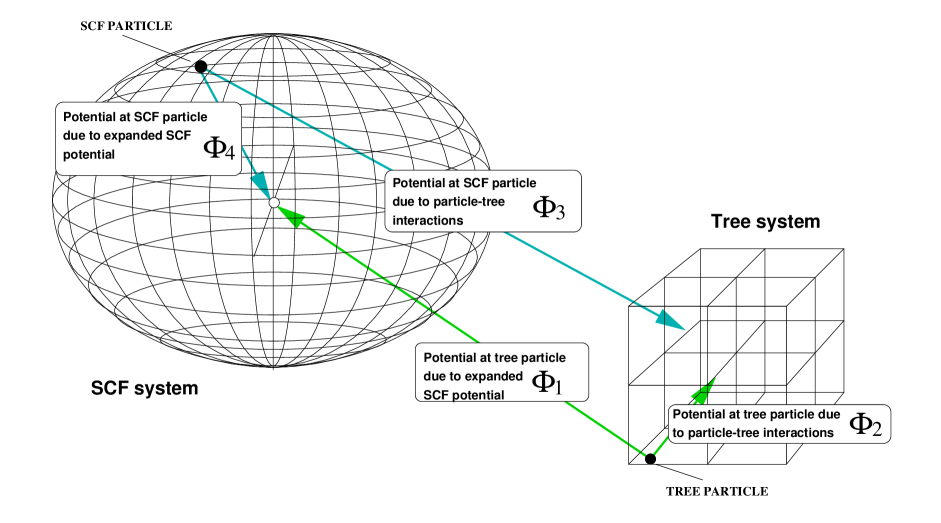
Figure 1: Schematic representation of the interaction between the SCF system and Tree system. The potentials $\Phi_{1}$ and $\Phi_{4}$ are due to the expanded SCF potential, see equation (12), at a position relative to the centre of mass of the SCF system (as defined in §2.3). The potentials $\Phi_{2}$ and $\Phi_{3}$ are due to the tree system of particles. The calculation of the tree potential is described in §2.1.

2.2 Self-Consistent Field Code

As far as a star in a galaxy is concerned, the dominant component of the gravitational potential which it experiences comes from the averaged field of billions of distant gravitational sources. It may appear rather odd that on the whole, the simulation of the gravitational dynamics of galaxies employs a method of basically summing up all the individual particle–particle interactions, each one of which is just about negligible. The expansion techniques described in §1.2 appear more natural, as the force calculation on each particle considers the effect of the mean gravitational field of the whole system directly acting on the particle. One might expect that the effects of two-body relaxation would be ostensively mitigated. On the other hand the model system still consists of many fewer bodies than a real system, and thus the statistical fluctuations brought about by the finite number of particles will cause the expanded gravitational field to fluctuate and thus the overall effect on the system approaches that of one that has experienced a corresponding amount of two-body relaxation. The major advantage of the SCF method is that the speed of the computation scales as ${\cal O}(N)$. Therefore it is possible to increase the practical limit on the number of particles, $N$, and thus any statistical fluctuations in the expanded potential are reduced.

The principle behind the SCF approach is to represent the potential of the system as a truncated series of terms of an expanded set of basis functions. It is possible to find the coefficients of such an expansion from the known density field ‘sampled’ by the particles. Poisson’s equation is solved for the set of basis functions, and coefficients of the expanded potential can be found. From the potential expansion the acceleration of any particle can be directly calculated. This technique had been applied in various guises and various degrees to a limited extent in the past [Clutton-Brock 1973, van Albada & van Gorkom 1977, McGlynn 1984]. The philosophy behind the SCF method of Hernquist & Ostriker (1992) was to use a set of basis function where the lowest order terms well represent the observed distribution in spheroidal galaxies. This method has subsequently been successfully utilised in further studies, [e.g. Johnston, Spergel, & Hernquist (1995); Hozumi & Hernquist [Hozumi & Hernquist 1995], Hernquist, Sigurdsson, and Bryan [Hernquist et al. 1995], Sigurdsson, Hernquist, & Quinlan [Sigurdsson et al. 1995]]. Below we present a quick resumé of the method of [Hernquist & Ostriker 1992].

Hernquist [Hernquist 1990] demonstrated that a density-potential pair exists such that their properties provide a very good approximation to the actual properties of observed galaxies, i.e. the $R^{1/4}$ law. They are:

$$\rho(r)=\frac{M}{2\pi}\frac{a}{r}\frac{1}{(r+a)^{3}};$$ (9)

and

$$\phi(r)=-\frac{M}{r+a}.$$ (10)

The total mass is $M$, and $a$ is the scale length related to the half-mass radius such that $r_{1/2}=(1+\sqrt{2})a$. A great advantage of this density–potential pair is that many of its properties can be derived analytically.

A biorthogonal basis set is constructed for the density and the potential, and they can be written as expanded series:

$$\rho({\mn@boldsymbol{r}})=\sum_{nlm}A_{nlm}\rho_{nlm}({\mn@boldsymbol{r}}),$$ (11)

and

$$\Phi({\mn@boldsymbol{r}})=\sum_{nlm}A_{nlm}\Phi_{nlm}({\mn@boldsymbol{r}}),$$ (12)

where $n$, $l$, and $m$ are equivalent to “quantum” numbers in the expansion, one radial, and two angular. Each pair $\rho_{nlm}$ and $\Phi_{nlm}$ satisfy Possion’s equation (3).

The lowest order terms are set to be those of the assumed model, i.e. $\rho_{000}\equiv\frac{1}{2\pi}\frac{1}{r}\frac{1}{(1+r)^{3}}$ and $\Phi_{000}\equiv-\frac{1}{1+r}$, where $G=M=a=1$. It is possible to construct the higher order terms of the expanded potential-density series $\Phi_{nlm}({\mn@boldsymbol{r}})$ and $\rho_{nlm}({\mn@boldsymbol{r}})$, and to derive an expression for calculation of the coefficients $A_{nlm}$. The interested reader may refer to the clear presentation given in Hernquist & Ostriker [Hernquist & Ostriker 1992].

Once all the $A_{nlm}$ have been calculated from the known coordinates of all the particles, the potential at the location of any particle can be evaluated using equation (12), and thus the acceleration of the particle can be found using equation (5).

For the purposes of our hybrid code, the basis set derived by Hernquist & Ostriker (1992) is an ideal choice. Other basis sets may be more useful for other systems such as discs, or objects that are not well-approximated by the $R^{1/4}$ profile. [Other basis sets are discussed elsewhere e.g. Saha (1993); Earn (1995); Earn & Sellwood (1995); Zhao (1996); Syer (1995)]

2.3 Combining Tree and SCF

The problem we are faced with is how to combine the two codes. It is a relatively simple task, all we need to achieve is

$${\mn@boldsymbol{a}}_{\mathrm{(}on\,tree\,particle)}={\mn@boldsymbol{a}}_{\mathrm{(}due\,to\,Tree)}+{\mn@boldsymbol{a}}_{\mathrm{(}due\,to\,SCF\,expansion)},$$ (13)

$${\mn@boldsymbol{a}}_{\mathrm{(}on\,SCF\,particle)}={\mn@boldsymbol{a}}_{\mathrm{(}due\,to\,SCF\,expansion)}+{\mn@boldsymbol{a}}_{\mathrm{(}due\,to\,Tree)}.$$ (14)

The left-hand sides of equations (13) and (14) are the total accelerations on a particle in the TREE and SCF systems respectively. The first terms on the right hand side are the accelerations on the particles due to their own systems, the terms on the far right are the extra accelerations due to the other system of particles. This is schematically shown in Figure (1).

When implementing this there are a couple of points to bear in mind. Firstly we need to take account of the response of the SCF system as a whole to the TREE system, i.e. the centre of mass will not be fixed. So we have to make sure that the SCF expansion is calculated about the centre of mass, or symmetry, of the SCF system of particles. As the SCF system evolves it may become asymmetric to some degree, hence we need to ensure that the expansion takes place about the most tightly bound region. We achieve this by calculating the centre of mass only from the contribution of particles which have less than the average particle energy. This is a parameter which may affect the accuracy of the expansion. It is possible to vary the energy level cut off for calculation of centre of mass. We discuss this further in §3.5.

Our concern now is how to treat the Tree system of particles with respect to the individual SCF particles. There are two options. Firstly, we may perform an expansion of the tree system much in the same way as the SCF system, then each SCF particle will view the potential due to the Tree system as a truncated set of terms in an expanded potential. For encounters that are non-penetrating this may prove a quick and reasonable approximation, but because the tree system is a priori not assumed to have any particular geometry, and likely to have a widely disrupted one, we would not expect it to be accurately represented in just a few terms of an expanded potential. Since we also desire our models to describe encounters and interacting systems we have to be aware that particle-particle interactions would not be accounted for if we used an SCF expanded Tree potential, e.g. the effects of dynamical friction would be poorly represented. Our other, more instinctive, option is to treat the system of Tree particles simply as a tree from the point of view of the SCF particles. This is a much more logical procedure as the tree has already been constructed and all that needs to be done for each SCF particle is to construct a tree interaction list and then sum the over particle-cell forces in the list.

The main calculations performed by the code in each time step of the system are outlined in the following sections.

2.3.1 Expansion Centre of the SCF System

As stated above the centre of mass of the SCF system is updated every timestep. Its position is calculated from the most tightly bound particles and is subsequently used as the origin of the SCF expansion when producing the coefficients, $A_{nlm}$.

2.3.2 Tree Particle – SCF Interaction

The position of each tree particle, ${\mn@boldsymbol{r}}\rightarrow(r,\theta,\phi)$, with respect to the SCF expansion centre, is passed to a routine which calculates $\Phi({\mn@boldsymbol{r}})$, i.e. equation (12). The $A_{nlm}$ have been already found for the case of the SCF system. The resulting acceleration of the Tree particle due to the SCF system is subsequently calculated.

2.3.3 Acceleration of Tree Particles due to Tree

As described in §2.1, a tree data structure is built from the particles in the tree system. Then for each particle an list of interactions between itself and the tree cells is formed subject to the tolerance parameter, $\theta$. Finally the cell-particle accelerations for each element in the list are calculated, summed, and added to the SCF acceleration from §2.3.2.

2.3.4 Acceleration of SCF Particles due to SCF

As described in §2.2 the coefficients, $A_{nlm}$, of the SCF expansion are calculated from the positions of the SCF particles. The acceleration due to the SCF system on each SCF particle is then found by applications of equations (12) and (5).

2.3.5 SCF Particle – Tree Interaction

For each SCF particle we build a tree interaction list. Each level of tree cells from the largest (root) to the smallest (single particle) is examined. If the criterion of inequality (8) is satisfied then the cell is added to the interaction list, otherwise the next level down is examined. Once the interaction list is formed, the list is looped through, summing the accelerations between the SCF particle and the tree cell as calculated by equation (7), and adding this to the acceleration due to the SCF particles themselves.

2.3.6 summary

For each timestep:

1. Find centre of mass of SCF system to use as centre
            of expansion.

2. Calculate the coefficients $A_{nlm}$ of the terms in the
             SCF expansion.

3. Build the Tree from all the Tree particles
   

4. For each Tree particle:
             a) Calculate $\Phi_{SCF}(\mn@boldsymbol{r}_{Tree})$.
             b) Form Tree interaction list between TREE particle
                 and Tree system subject to $\theta$.
             c) Calculate $\Phi_{Tree}(\mn@boldsymbol{r}_{Tree})$.
             d) Calculate acceleration of Tree particle.

5. For each SCF particle:
             a) Calculate $\Phi_{SCF}(\mn@boldsymbol{r}_{SCF})$.
             b) Form Tree interaction list between SCF particle
                 and Tree subject to $\theta$.
             c) Calculate $\Phi_{Tree}(\mn@boldsymbol{r}_{SCF})$.
             d) Calculate acceleration of SCF particle.

6. Update positions and velocities of all particles.

2.4 Implementation

The aim in this project was to combine two separate codes into one hybrid code. The process was made much easier by the availability to us of optimised versions of both the treecode and SCF code written in Fortran 77. We acknowledge the author, Lars Hernquist, for making these codes freely available.

The two codes were made compatible and carefully purged of any overlapping routines and variables ensuring no cause for confusion existed. The extra routines added were: calculation of the SCF system centre of mass correction; formation of tree interaction list for an SCF particle; calculation of the acceleration on a SCF particle from the tree list; calculation of the acceleration on a Tree particle from the SCF expanded potential; and a number of modifications to the output information.

The final version of the SCFTREE code was implemented on a Sun Sparc20 workstation running Solaris 2.4, and being written in standard F77 should be fully portable.

3 Tests

Having two sets of particles that are evolved under two different numerical schemes one has to be very careful that the system as a whole is behaving as a realistic model of the system it represents. We conduct a variety of stringent tests on accuracy and efficiency which display the applicability of this code to the systems it was designed to deal with. In this section we quantify the efficiency of the code, check its validity with respect to the constants of motion, and put its performance to the test in a number of dynamical examples.

3.1 Models

Three distributions of particles are realised in order to test the stability of spherical systems and compare the ability of SCFTREE to handle distributions departing from the Hernquist distribution (the SCF basis set). The distributions are the Hernquist density profile [Hernquist 1990], the Plummer density profile [Plummer 1911], and the Lowered Evans model [Evans 1993]. The Lowered Evans model has been shown to be useful for the practical modelling of dark halos [Kuijken & Dubinski 1994], and as such is our preferred model in many of the tests. With reference to the parameters in Kuijken & Dubinski (1994) we use the following for all our Lowered Evans models: $\Psi_{0}=-5.0$, $v_{0}=1.5$, $q=1.0$, $(r_{c}/r_{k})^{2}=1.0$, $r_{a}=1.0$.

In these tests the models are populated with up to $10^{5}$ particles and a specified fraction of them are designated as particles to be dealt with by the Tree part of the code, referred to hereafter as ‘Tree particles’. The remainder of the particles are dealt with by the SCF part of the code and referred to as ‘SCF particles’.

Analogous to the investigations of Hozumi and Hernquist [Hozumi & Hernquist 1995] who perform tests on the pure SCF code, we examine the behaviour of SCFTREE in systems which are not in equilibrium. For this purpose we construct a uniform density sphere with velocity dispersions assigned according to a specified initial virial ratio, the evolution of the system is followed until it reaches its final relaxed state.

Extending these tests of SCFTREE to more interesting systems we perform test runs on a disk system. A disk, bulge, and halo model is set up as prescribed in Dubinski and Kuijken (1995). Such a system is well suited to the SCFTREE technique whereby the disk particles are assigned to the Tree and the halo and bulge particles are assigned to the SCF system. Here we merely examine the effect of increasing the number of halo particles on the stability of the disk.

Figure 2: CPU per timestep performances for SCFTREE.
(a) SCFTREE is compared to pure Tree and pure SCF codes, in the SCFTREE runs 10% of the particles are designated as Tree particles and distributed randomly through the system (A lowered Evans model with 20000 particles, dt=0.05).
(b) Binary system of spherical galaxies in a circular orbit. Mass ratio 10:1. In the SCFTREE runs the smaller satellite is composed of only Tree particles and the larger body composed of only SCF Particles.
(c) Variation of the fraction of Tree particles, $N_{\rm tree}/N_{SCF}$ distributed randomly in a Lowered Evans model.

3.2 Timing

The individual timing performances of tree and SCF codes have been shown to scale to ${\cal O}(N_{tree}\log N_{tree})$, [Barnes & Hut 1986], and ${\cal O}(N_{SCF})$, [Hernquist & Ostriker 1992], respectively. For the combined code we have to consider the CPU time spent on the interaction between the two components. The calculation of the Tree force on each SCF particle would, at worst, scale as ${\cal O}(N_{SCF}\log N_{tree})$, and that of the SCF force on the tree particles scales as ${\cal O}(N_{tree})$. So overall we would expect the CPU time to scale as

$${\cal O}\left[N_{SCF}(1+\log N_{tree})+N_{tree}(1+\log N_{SCF})\right].$$ (15)

As the major advantage of SCFTREE is expected to be its efficiency in dealing with systems with substructure, we perform tests varying the fraction of tree particles in the system and changing the initial distribution of these particles. The models used here for the performance checks are the Lowered Evans models.

We examine how the timing of SCFTREE behaves with the total number of particles. The fraction of tree particles is set at 10% of the total and they are distributed randomly throughout the system. The random distribution of particles implies that there will not be any advantage in time saved due to the Tree structure. This is demonstrated in Figure 2(a) where we compare purely Tree, purely SCF, and SCFTREE timings as the total number of particles is increased up to $10^{5}$. As expected no advantage is offered by SCFTREE with randomly distributed particles over the pure Tree treatment.

The great advantage of SCFTREE is demonstrated in Figure 2(b) where the Tree particles are assigned to a satellite system orbiting a more massive system composed of the SCF particles. This is compared to a pure Tree treatment of the same binary system. The Figure clearly demonstrates the strength of SCFTREE when the Tree particles are assigned to a distinct substructure. We see that for SCFTREE the CPU time per timestep scales approximately as ${\cal O}(N)$, a substantial improvement over the pure Tree timings.

Finally we examine the performance of the code as the fraction of Tree particles is increased. Figure 2(c) shows the CPU time spent both on the whole SCFTREE timestep and just on the Tree timestep in a system with a randomly distributed fraction of Tree particles. It can be seen that for such a system the fraction of Tree particles must remain below $\sim 10$% to gain any reasonable advantages.

3.3 Relaxation

Figure 3: The magnitude of 2-body relaxation in the system versus time. The relaxation measure we use is $\left<|\Delta E/E|^{2}\right>$, defined in equation (16). The model is a Lowered Evans model containing 20,000 particles, 10% being randomly distributed tree particles.

Figure 4: An example of the total fractional energy change, $(E_{t}-E_{0})/E_{0}$, as a function of time, for a Lowered Evans model, 20000 particles with 10& in Tree. SCF truncation parameters are $n=16$ and $l=6$. SCFTREE conserves energy to within duration of this run.

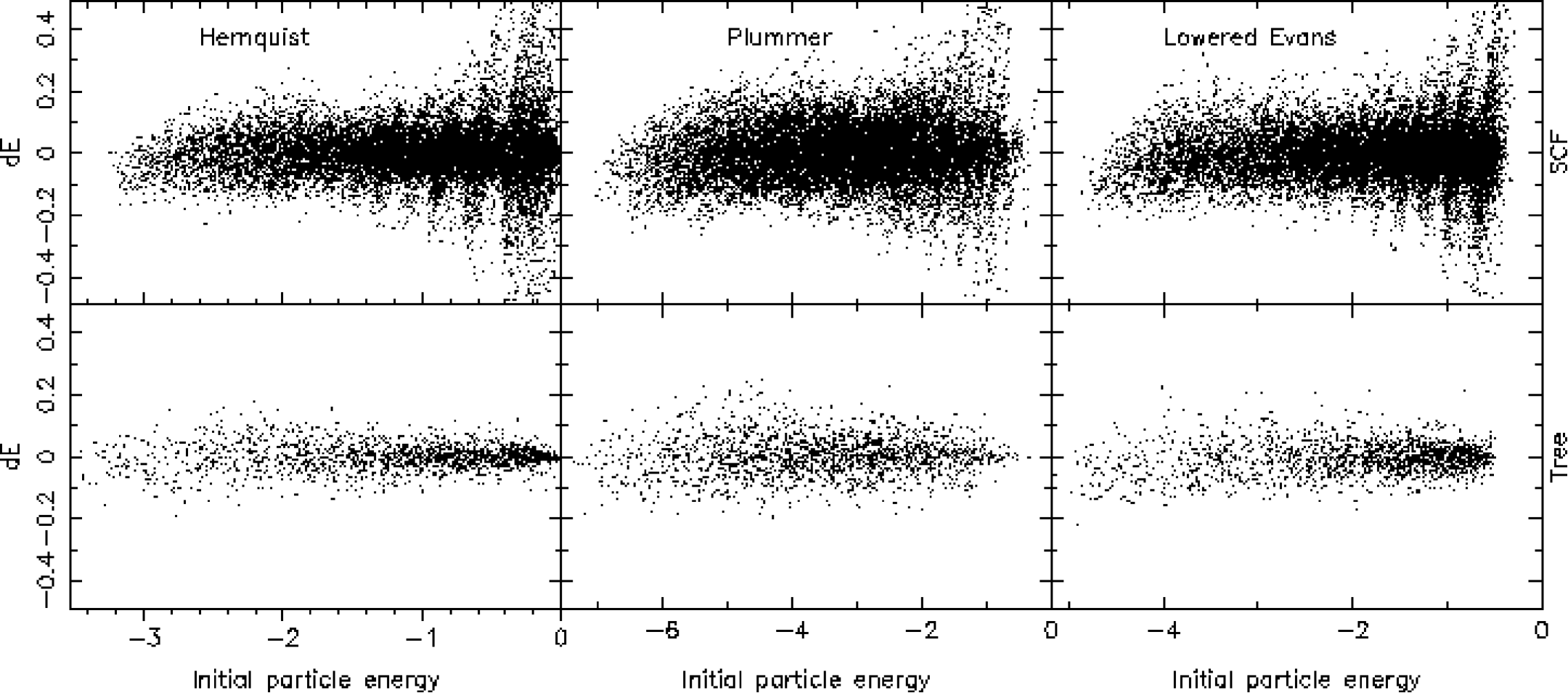
Figure 5: How the individual particle energies behave with respect to different initial equilibrium models. Results are calculated from $t=10$ to $t=50$. All models consist of a total of 20000 particles, 2000 of which are randomly assigned to the Tree system. The SCF expansion is truncated at $n=6$ and $l=2$.

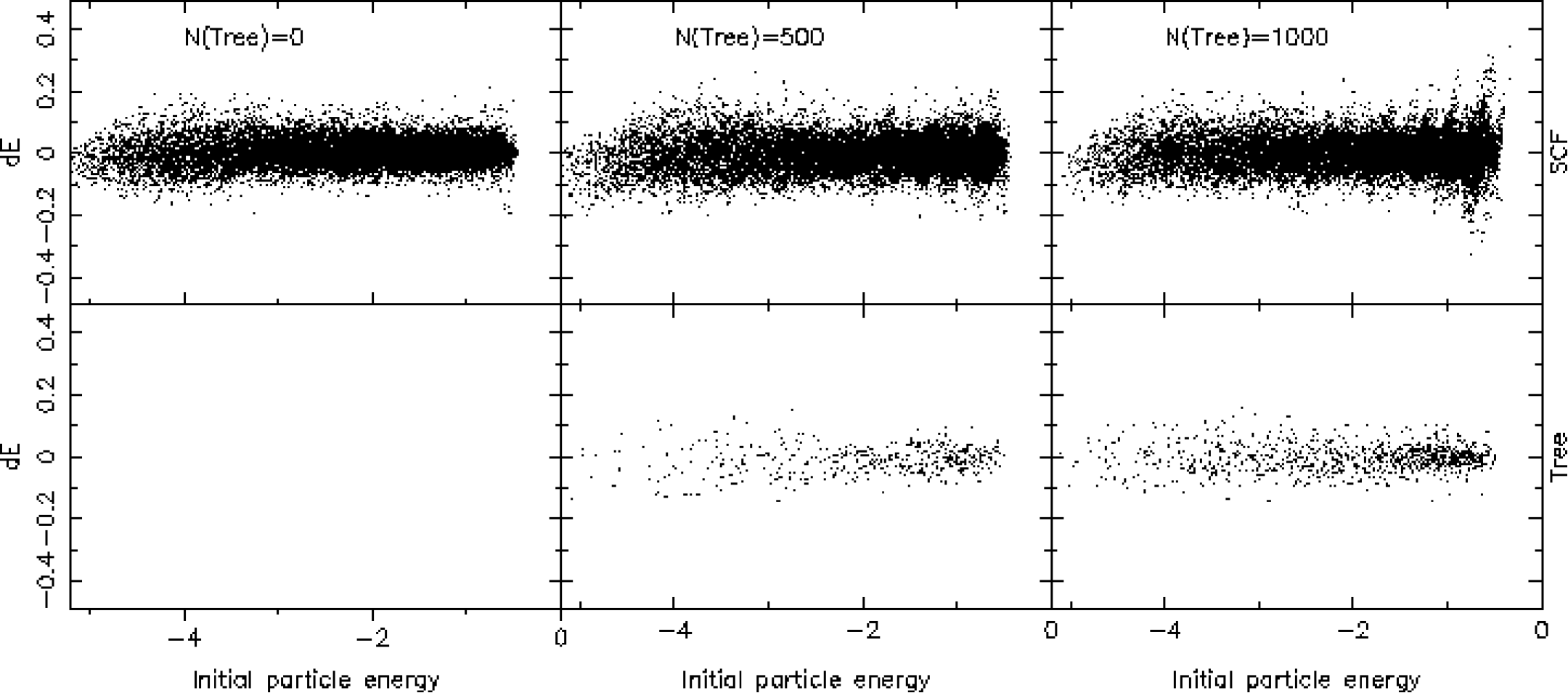
Figure 6: Showing the effect on individual particle errors as the fraction of Tree particles in the simulation is reduced. This demonstrates that it is the presence of the Tree particles in the system which cause the vertical “bands” associated with certain energies. The relative energy difference per particle, $dE$, is calculated from $t=10$ to $t=50$. These models are Lowered Evans models with a total of 20000 particles.

It is instructive to follow the behaviour of two-body relaxation as the system evolves. As an indicator of two-body relaxation we take the mean square fractional energy change of the particles, $R_{2-body}=\left<|\Delta E/E|^{2}\right>$. We define this as

$$R_{2-body}=\frac{1}{N}\sum_{i=1}^{N}\left|\frac{E_{i,t}-E_{i,0}}{E_{i,0}}\right|^{2},$$ (16)

$E_{i,t}$ and $E_{i,0}$ are the total energy (kinetic plus potential) of particle $i$ at times $t$ and 0 respectively. In Figure (3) we see that by our measure the average relaxation remains less than $1\%$ for the period of the simulation. The initial sharp rise is expected due to the initial random placing of the particles, meaning that many pairs of particles will have initial separations less than the tree softening length, $\epsilon$.

3.4 Energy Conservation

Relaxation tells us how close our models approach the behaviour of a collisionless system, providing us with a quantitive estimate of over what timescales our simulations can be applied.

We may also look at the change in the energy of each particle over a suitable time period and compare the behaviour of SCF and tree particles. This gives another gauge of relaxation of particles this time as a function of the binding energy, $E$. We follow a similar analysis as HO92 and plot $\Delta E/E$ vs $E$ for both SCF and tree particles. Figure(5) shows the results for the 3 spheroidal models: Hernquist; Plummer; and Lowered Evans. Each model is populated with 20000 particles and the energy change is fractional difference of the particle energy at times $t$ and $t_{0}$. One will notice all three SCF particle plots exhibit a vertical band structure at certain binding energies. The cause of some particles being more liable to undergo two-body relaxation than other is made clearer by Figure(6) which shows the same plots for three Lowered Evans models with 0, 500, and 1000 tree particles respectively. The greater the fraction of tree particles the wider and more distinct the vertical features that appear in the regions of low binding energies. The first point to bear in mind is that at low energies the fractional energy changes will become large because the binding energy is approaching zero. Secondly it is clear that greater the number of tree particles the greater the fractional energy change. This is due to the fact that individual SCF particles interact directly with the tree particles, and so the more tree particles the greater the energy exchange between the two components. Finally the bands that are seen appear as a result of truncating the SCF expansion. The expanded potential of the system is derived from the actual positions of all the constituent SCF particles. The actual binding energy of a particle may not agree exactly with the potential given by the expansion, causing an error in the resulting acceleration. There will be certain values of binding energy which correspond to the divergences in the truncated expanded potential from the true value, thus the particles at those binding energies will experience greater errors in acceleration. Clearly the presence of Tree particles in the system exacerbates this effect. However because these effects are symmetric the overall global errors remain minimal.

This is confirmed by monitoring the total energy of the system. Figure(4) traces the fractional variation in total energy of the system, $(E_{t}-E_{t_{0}})/E_{t_{0}}$. The model is a Lowered Evans with 20000 particles, 10% being Tree particles, and timestep $dt=0.05$. Energy is conserved in this system to within 0.8% over a period of 50 time units.

3.5 Momenta

Figure 7: Plot (a) shows the relative angular momentum change, $(|L_{t}|-|L_{0}|)/|L_{0}|$, with time. Plot (b) shows the evolution of the z-component of the angular momentum, $L_{z}$, with time. The data is from a Lowered Evans model containing 20,000 particles, 10% of which are tree particles.

As with all expansion codes angular and linear momentum are intrinsically not conserved exactly, due to approximations in the force calculation. We might expect it to be more pronounced in the SCFTREE case where the particles in the Tree and SCF codes do not respond to each other equally and oppositely. Linear momentum is known not to be conserved in the pure SCF case, and can be taken care of by recentering the particles. In this case, every expansion of the SCF system is taken about its centre of mass, alleviating the need to recentre the particle. We check the accuracy of this modification by monitoring the conservation of linear momentum of the SCF centre of mass of a spherical stellar system, and the separation of a binary system of spherical galaxies (one SCF; one Tree) in a circular and stable orbit. Figure 10 shows the separation between an SCF and a Tree spheroid of equal mass, both with 2500 particles, in a circular orbit.

We show an example of the evolution of the total angular momentum of the system in Figure (7a) and although $|{\bf L}|$ is intrinsically near zero we see that it varies no more than 1% over the length of the run. Figure (7b) shows the absolute variation of the $z$-component of ${\bf L}$. The system in this case is a Lowered Evans Model with 20000 particles with 10% Tree particles.

3.6 Collapse of uniform sphere

We investigate the performance of the SCFTREE code on a system which is not initially in equilibrium. For this purpose we perform simulations on the collapse of a uniform density spherical distribution of particles with random velocities scaled such that the initial virial ratio of the system $\left|2T/W\right|_{0}=1/2$. Following the thorough investigation by Hozumi and Hernquist (1995) of the pure SCF code in similar non-equilibrium states, we trace the evolution of the virial ratio from its initial value of $1/2$. Our purpose here is not to perform a detailed investigation of the accuracy of the dynamical evolution but as a qualitative check that the combined SCF and Tree codes behave as expected, and the virial ratio oscillates about the equilibrium value of $\left|2T/W\right|_{0}=1.0$. The results are shown for a typical run containing 20000 particles, 10% of which are randomly allocated as tree particles. The truncation parameters for the SCF part are $n=16$ and $l=6$.

Figure(8) shows the plot of final density profile of the same system after a period of $t=120$. The separate profiles of the Tree and SCF systems of particles are shown, together with the total profile of all of the particles. In the example shown the system undergoes homologous collapse (Fillmore & Goldreich 1984; Gunn 1977) evolving to a density profile of $\rho\sim r^{-2.5}$. Towards the core of the system in this example the number of particles is too small to adequately resolve the detailed evolution (cf. Hozumi & Hernquist (1995) who used hundreds of thousands of particles and obtained adequate resolution to resolve the flattening of the core.)

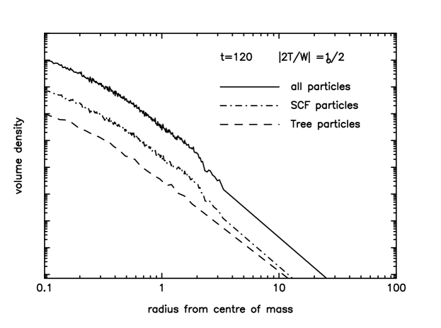
Figure 8: Final density profile after $t=120$ of the collapsed sub-virial ($|2T/W|_{0}=\frac{1}{2}$) uniform density sphere. Density profiles are individually shown for the SCF and Tree components, shifted vertically for comparison.

Figure 9: The viral ratio, $|2T/W|$, evolution of the collapse of a subvirial uniform density sphere. The total number of particles is 20000, with a random 10% being assigned to the Tree system.

Figure 10: This plot shows the absolute separation between two non-penetrating systems in circular orbit around each other. Each system is an identical Lowered Evans model populated with 2500 particles. One is assigned to the SCF system, the other to the Tree system. This figure demonstrates that the method of expanding the SCF potential around its centre of mass every timestep remains accurate to within 5% over 400 time units.

3.7 Disk + Halo + Bulge

We have seen from the previous tests that the code is efficient and accurate even when the tree particles are random distributed amongst the SCF particles. This is the worst case scenario in terms of efficiency. During the force calculation on an SCF particle it will form a large list of tree cell interactions. Now we move to a case where the tree particles form some distinct structure within the SCF system, that of a disk embedded within a halo. The study of disk evolution in a non-interacting system has been the focus of much research and requires a good deal more attention than a mere subsection to investigate it fully. Here we content ourselves with an example of how the varying of $N_{\rm halo}$ affects the stability of the disk. We construct combined disk–halo–bulge models using the method of Dubinski & Kuijken (1995). The ratio of masses of the components was disk:bulge:halo = 1.00:0.37:12.80, the scale radius of the disc was set to $R_{d}=1.0$. The number of disk particles in each case was 6000, and the number of bulge particles was 2000. In four runs the number of halo particles was varied from 13000 to $10^{5}$. Each time the disk particles were assigned to the Tree system and the rest to the SCF system.

Figure 12 demonstrates increased stability as number of halo particles, $N_{\rm halo}$ is increased. In particular at $N_{\rm halo}=100000$ little structure has formed in the disk and is unchanged apart from a slight thickening, whereas for $N_{\rm halo}=13000$ the disk is particularly unstable to warping, and spiral structure seems to be developing. The thickening of the disk shown in Figure 11. These figures confirm what we would expect as we change the number of $N_{\rm halo}$ in a self-consistent simulation. With fewer SCF particles noise in the SCF expanded potential will cause fluctuations in the halo potential to develop, and thus cause the disk to become unstable to warping.

Figure 11: Vertical velocity dispersion, $\sigma_{z}$ and rms disk height, $z_{\rm rms}$ as a function of radial distance at $t=120$. The construction of the disk–halo–bulge models is described in §3.7. The three different runs correspond to the curves (a), (e), and (b) in Figure 12.

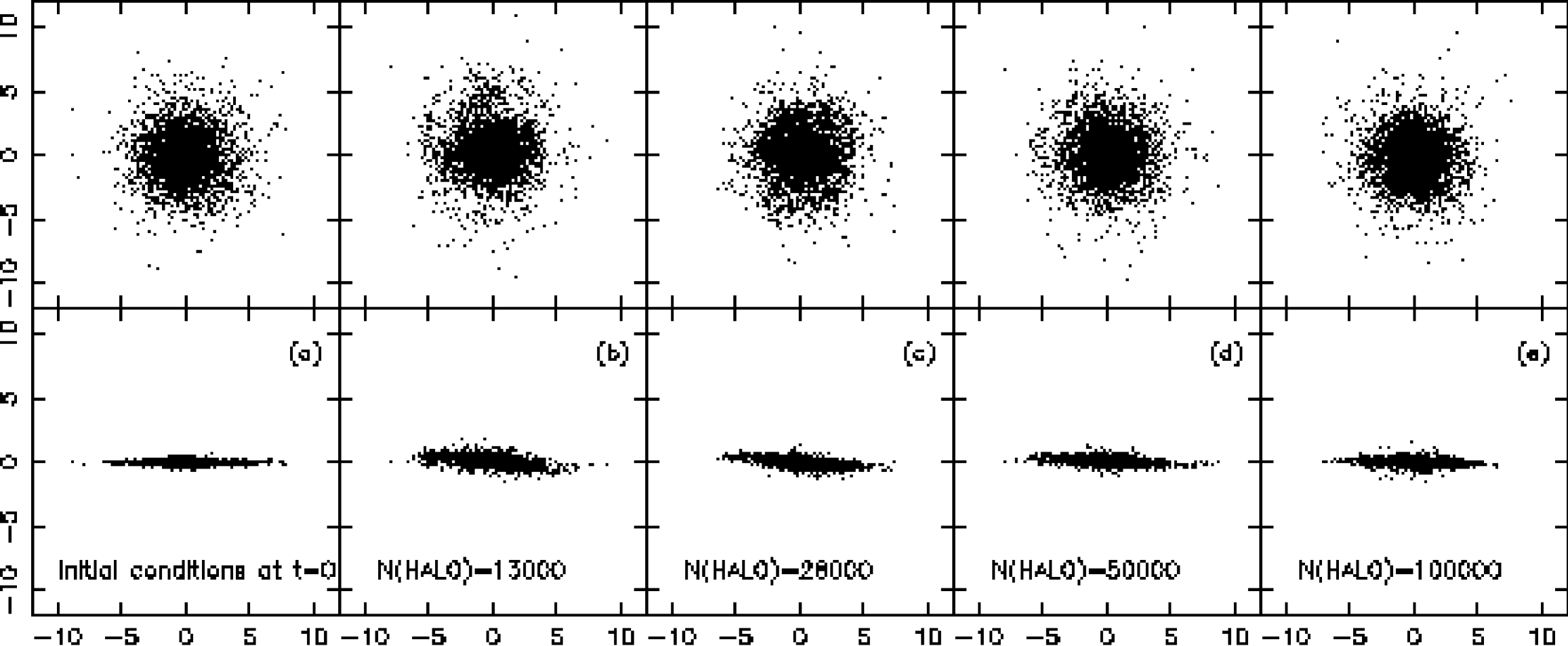
Figure 12: This figure plots the Tree particles only after $t=120$ to show the effect of changing the number of particles in the halo i.e. the SCF particles, on the stability of the disk. The construction of the models is described in §3.7. The initial conditions are shown in plot (a), with the numbers of particles in the Halo increasing to the right. The top row and bottom row show the x-y plane and the y-z plane respectively.

3.8 Dynamical Friction

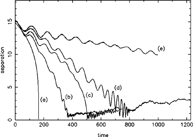
Figure 13: The decay in separation between a massive spherical primary, treated by the SCF system, and a smaller spheroidal satellite, treated by the Tree system. The models used for each curve are summarised in Table 1. As discussed in §3.8 this figure demonstrates the effectiveness of using SCFTREE to model dynamical friction.

Penetrating encounters between stellar systems provide many interesting scenarios which one could fruitfully model with our hybrid code. Representing interacting systems separately with the SCF and Tree methods invites the question of how well SCFTREE describes the behaviour of SCF and Tree particles interacting with each other in differing ways. We address this issue by investigating the ability of the code to tackle dynamical friction, specifically by running a few simulations of the sinking satellite sort. SCF is used to model the primary, and Tree used for the satellite. Although the force on each SCF particle due to the Tree particles is directly calculated (subject to the tolerance criterion), the Tree particles only respond to the SCF particles indirectly via the expanded field. One might initially be concerned that the lack of direct particle–particle interactions which account for the deceleration of the satellite will invalidate the use of this code in such cases, however we show that so long as the SCF expansion is truncated after a reasonable number of terms dynamical friction is acceptably treated.

Model	$N_{\rm primary}$	$N_{\rm satellite}$	SCF truncation
(a)	Approximate analytical solution valid for large r
(b)	20000	1000	$n=16$	$l=6$
(c)	20000	1	$n=16$	$l=6$
(d)	20000	1000	$n=8$	$l=2$
(e)	20000	1	$n=8$	$l=2$
Primary:	Hernquist model; $R_{a}=1$; $R_{\rm max}=200$; $M=7.39$
Satellite:	LE model; $R_{a}=0.1$; $R_{\rm max}=3.6$; $M=0.75$
Initial separation on circular orbits =15

Table 1: Summary of the models and model parameters used in the tests of dynamical friction

Figure(13) demonstrates the dependence of dynamical friction on the number of expansion coefficients used in the expanded SCF potential. The initial conditions and the models used to represent the primary and satellite are summarised in Table 1. Curve (a) in the Figure is a simple analytical approximation of the sinking rate based on the Chandrasekhar dynamical friction formula [Binney & Tremaine 1987]. We approximate $f(0)=$constant, and assume instantaneously circular orbits for the satellite. This calculation carries with it the assumption of a fixed primary and is valid only in the region of large separations, $r$, low circular velocity, no satellite mass loss, and is to be disregarded at small $r$.

As one might expect when the SCF expansion is truncated at low orders [curves (d) and (e)] dynamical friction is poorly modelled. Increasing the truncation order [curves (b) and (c)] with a corresponding increase in the resolution of the SCF system causes the Tree system to respond realistically to perturbations in the SCF density field. With the SCF expansion truncated at $n=16$ and $l=6$ and taking a single point mass for the satellite (i.e. one tree particle) dynamical friction is modelled well (see curve [c]). We find these sinking times are consistent with the results obtained by Hernquist and Weinberg (1989) for fully self-consistent simulations using a pure tree code and concur with their findings [and of White (1983)] that when the response of the primary is included in the numerical calculations the sinking time increases by a factor of around two.

Decay of the orbit of a single point mass means in simple terms that orbital energy is transferred to dynamical heating of the particles in the primary. For an extended satellite (i.e. one composed of $N_{satellite}$ bodies), orbital energy can also be transferred to the heating of the satellite, thereby increasing the decay rate and shortening the decay period. This interesting result is demonstrated in curve (b), and certainly warrants greater detailed exploration. The result has been clearly alluded to in Weinberg (1989) in terms of coupling in the analytic linear theory which he describes. The extended satellite has many weak resonances which can couple at smaller radii, which the point mass does not.

Finally we note that the sinking satellite loses much of its mass during its descent. For the example traced by curve (b) in Figure(13), 40% of the Tree particles become unbound from tree system at $r\sim 7$, and 80% are unbound at $r\sim 2$. The peculiar behaviour of the curves once having reached $r\sim 1$ is due to the practical disruption of the satellite.

4 Discussion

In this paper we have presented SCFTREE, a hybrid N-body code combining the Hernquist & Ostriker Self–Consistent Field code, and the Barnes–Hut hierarchical tree algorithm. The SCF code is designed to model systems with structure resembling to first order the Hernquist density profile, $\rho(r)\propto\frac{1}{r(r+a)^{3}}$. The treecode technique is a proven approach to effectively model systems that have no a priori and in effect, no limit to dynamical or spatial range. The principle behind the SCFTREE scheme is to model evolving structures that interact with or are within an approximate Hernquist potential. The uses of such an approach are wide ranging, especially modelling the evolution of structures within a dark matter halo, e.g. disks, bars, satellite galaxies, interactions and encounters, and cluster galaxies within a cluster halo.

The prime advantage of this new technique is a significant improvement in performance over using pure treecodes which scale as $\cal O(N\log N)$. To date only treecode techniques have been adequately suited to systems with such large dynamical ranges. However, so much CPU time is expended on parts of the system with little dynamical evolution such as the halo. By representing the halo with the SCF technique, where the CPU time scales as $\cal O(N)$, we are able to reduce the overall CPU time and thus can increase the total number of particles.

As this implementation of the code is based around global geometries which behave approximately as $R^{1/4}$ in projected density, its use would not be appropriate to model objects with substantially different density profiles. As mentioned in §2.2 other basis expansions for different mass distributions are possible. However, there are many systems that may be modelled by appropriate application of SCFTREE.

This implementation of SCFTREE is able to accurately model effects of dynamical friction and thus the application to systems of sinking satellites is a prime application. Other eminently suitable applications will be the evolution of inclined disks in flattened halos [Dubinski & Kuijken 1995], the evolution of unstable high-surface-density disks (Dalcanton et al. 1996; Vine & Sigurdsson 1997, in preparation), and weak encounters between massive elliptical systems and smaller disk systems (Vine 1997, in preparation).

This preliminary version of the code has much potential for future development and expansion, especially in terms of performance. The nature of the SCF code makes it suitable for parallelisation [Hernquist et al. 1995] together with a vectorised version of the Tree code utilising heterogeneous systems. With the advent of parallelised Tree implementations a doubly parallel SCFTREE is a possibility.

An interesting development will be to experiment with multiple expansions of the SCF systems. With such a tool it will be feasible to model interactions between two or more large spheroidal systems. For example in the evolution of galaxy groups and multiple mergers [Weil & Hernquist 1996]. The principle of having more than one expansion centre has been exploited some time ago [van Albada & van Gorkom 1977].

Work currently in progress includes a powerful improvement to the algorithm presented here, that of swapping particles between the SCF and Tree system when one system becomes more appropriate then the other. For instance the disruption of a satellite composed of Tree particles could benefit from transfer of escapers to the main body of the SCF primary. Conversely, structure formation in $N>10^{8}$ cosmological simulations can have increased resolution by assigning increasing numbers of Tree particles to structures.

Another relatively simple development is to incorporate hydrodynamics into the Tree part of the code [Hernquist & Katz 1989]. This could be further extended to encompass star formation prescriptions [Mihos & Hernquist 1994]. Ultimately it is not unreasonable that the technique could be employed in cosmological simulations which are now capable of dealing with much more sophisticated physical processes [Katz, Weinberg, & Hernquist 1996]

References

- [Aarseth 1972] Aarseth, S. J., 1972, in Gravitational N-body Problem, IAU Colloquium No. 10, ed. M. Lecar, (Dordrecht: Reidel), p. 373.
- [Aarseth 1985] Aarseth, S. J., 1985, in Multiple Time Scales, ed. J. U. Brackill and B. I. Cohen (New York: Academic), p. 377.
- [Appel 1981] Appel, A. W., 1981, Undergraduate Thesis, Princeton University.
- [Barnes 1988] Barnes, J. E., 1988, ApJ, 331, 699.
- [Barnes 1992] Barnes, J. E., 1992, ApJ, 393, 484.
- [Barnes 1996] Barnes, J. E., 1996, in ”Formation of the Galactic Halo…Inside and Out”, eds. H. Morrison & A. Sarajedini, p. 291.
- [Barnes & Hut 1986] Barnes, J. E. & Hut, P., 1986, Nature, 324, 446.
- [Bartlett & Charlton 1995] Bartlett, R. E., & Charlton, J. C., 1995, ApJ, 449, 497.
- [Binney & Tremaine 1987] Binney J. J., Tremaine S., 1987, in Galactic Dynamics. Princeton, p.190.
- [Casertano & Hut 1985] Casertano, S. & Hut, P., 1985, ApJ, 298, 80.
- [Clutton-Brock 1973] Clutton-Brock, M., 1973, Ap&SS, 23, 55.
- [Cooley & Turkey 1965] Cooley, J. W. & Tukey, J. W., 1965, MathComp, 19, 297.
- [Couchman 1991] Couchman, H. M. P., 1991, ApJ, 368, L23.
- [Couchman et al. 1995] Couchman, H. M. P., Thomas, P. A., Pearce, F. R., 1995, ApJ, 452, 797.
- [Davé 1997] Davé, R., Dubinski, J., Hernquist, L., 1997, New Astron. preprint.
- [Dubinski 1996] Dubinski, J., 1996, New Astron., 1(2), 133.
- [Dubinski & Kuijken 1995] Dubinski, J. & Kuijken, K., 1995, ApJ, 442, 492.
- [Dubinski et al. 1995] Dubinski, J., Mihos, J. C., Hernquist, L., 1995, ApJ, 462, 576.
- [Dyer & Ip 1993] Dyer, C. C. & Ip, P. S. S., 1993, ApJ, 409, 60.
- [Eastwood & Hockney 1974] Eastwood, J. H. & Hockney, R. W., 1974, J.Comp.Phys, 16, 342.
- [Ebisuzaki et al. 1993] Ebisuzaki, T., Makino, J., Fukushiga, T., Taiji, M., Sugimoto, D., Ito, T., Okumura, S., 1993, PASJ, 45, 269.
- [Efstathiou & Eastwood 1981] Efstafthiou, G. & Eastwood, J. W., 1981, MNRAS, 194, 503.
- [Evans 1993] Efstafthiou, N. W., 1993, MNRAS, 260, 191.
- [Farouki & Salpeter 1994] Farouki, R. T. & Salpeter, E. E., 1994, ApJ, 427, 676.
- [Gelato et al. 1996] Gelato, S., Chernoff, D. F., Wasserman, I., 1996, preprint.
- [Goldstein 1980] Goldstein, H., 1980, Classical Mechanics, p.229, (Reading: Addison-Wesley).
- [Greengard & Rokhlin 1987] Greengard, L. & Rokhlin, V., 1987, J.Comp.Phys., 73, 325.
- [Hernquist 1987] Hernquist, L., 1987, ApJS, 64, 715.
- [Hernquist 1990] Hernquist, L., 1990, ApJ, 356, 359.
- [Hernquist & Barnes 1990] Hernquist, L. & Barnes, J. E., 1990, 349, 562.
- [Hernquist & Katz 1989] Hernquist, L. & Katz, N., 1989, ApJS, 70, 419.
- [Hernquist & Ostriker 1992] Hernquist, L. & Ostriker, J. P., 1992, ApJ, 386, 375.
- [Hernquist et al. 1995] Hernquist, L., Sigurdsson, S., & Bryan, G. L., 1995, ApJ, 446, 717.
- [Hernquist & Weinberg 1989] Hernquist, L. & Weinberg, M. D., 1989, MNRAS, 238, 407.
- [Hockney & Eastwood 1981] Hockney, R. W. & Eastwood, J. W., 1981, Computer Simulation Using Particles (New York: McGraw-Hill).
- [Hozumi & Hernquist 1995] Hozumi, S. & Hernquist, L., 1995, ApJ, 440, 60.
- [Huang et al. 1993] Huang, S., Dubinski, J., Carlberg, R. G., 1993, ApJ, 404, 73.
- [Jernigan 1985] Jernigan, J. G., 1985, in IAU Symposium 113, Dynamics of Star Clusters, ed. J. Goodman and P. Hut (Dordrecht: Reidel), p. 275.
- [Johnston et al. 1995] Johnston, K. V., Spergel, D. N., Hernquist, L., 1995, ApJ, 451, 598.
- [Kandrup et al. 1994] Kandrup, H. E., Mahon, M. E., & Smith, Jr., H., 1994, ApJ, 428, 458.
- [Katz, Weinberg, & Hernquist 1996] Katz, N., Weinberg, D. H., Hernquist, L., 1996, 105, 19.
- [King 1966] King, I. R., 1966, AJ, 71, 64.
- [Kuijken & Dubinski 1994] Kuijken, K. & Dubinski, J., 1994, MNRAS, 269, 13.
- [McGlynn 1990] McGlynn, T. A., 1990, MNRAS, 348, 515.
- [McGlynn 1984] McGlynn, T. A., 1984, ApJ, 281, 13.
- [McMillan & Aarseth 1993] McMillan, S. L. W. & Aarseth, S. J., 1993, ApJ, 414, 200.
- [Merzbacher 1970] Merzbacher, E., 1970, Quantum Mechanics, (Wiley: New York).
- [Mihos & Hernquist 1994] Mihos, C. J. & Hernquist, L., 1994, ApJ, 437, 611.
- [Miller & Smith 1980] Miller, R. H. & Smith, B. H., 1980, ApJ, 235, 421.
- [Olsen & Dorband 1994] Olsen, K. M. & Dorband, J. E., 1994, ApJS, 94, 117.
- [Plummer 1911] Plummer, H. C., 1911, MNRAS, 71, 460.
- [Porter 1985] Porter, D., 1985, PhD Thesis, University of California, Berkeley.
- [Salmon 1996] Salmon, J. K., 1996, ApJ, 460, 59.
- [Salmon 1991] Salmon, J. K., 1990, PhD Thesis, Califorina Institute of Technology.
- [Salmon & Warren 1994] Salmon, J. K. & Warren, M. S., 1994, J.Comp.Phys., 111, 136.
- [Schmidt & Lee 1991] Schmidt. K. L. & Lee, M. A., 1991, J.Stat.Phys., 63, 1223.
- [Sellwood 1987] Sellwood, J. A., 1987, ARA&A, 25, 151.
- [Sigurdsson et al. 1995] Sigurdsson, S., Hernquist, L., & Quinlan, G. D., 1995, ApJ, 446, 75.
- [Steinmetz 1996] Steinmetz, M., 1996, MNRAS, 278, 1005.
- [Steinmetz & White 1996] Steinmetz, M. & White, S. D. M., 1996, MNRAS, preprint.
- [Syer 1995] Syer, D., 1995, MNRAS, 276, 1009.
- [van Albada & van Gorkom 1977] van Albada, T. S. & van Gorkom, J. H.. 1977, A&A, 54, 121.
- [Walker et al. 1996] Walker, I. R., Mihos, J. C., & Hernquist, L., 1996, ApJ, 460, 121.
- [Warren & Salmon 1992] Warren, M. S. & Salmon, J. K., 1992, In Supercomputing ’92, (IEEE Comp. Soc.: Los Alamitos), p. 570.
- [Warren 1994] Warren, M. S., 1994, PhD Thesis, California University, Santa Barbara.
- [Warren & Salmon 1993] Warren, M. S. & Salmon, J. K., 1993, In Supercomputing ’93, (IEEE Comp. Soc.: Los Alamitos), p. 12.
- [Weil & Hernquist 1996] Weil, M. L., & Hernquist, L., 1996, ApJ, 460, 101.
- [Weinberg 1996] Weinberg, M. D., 1996, ApJ, 470, 715.
- [Weinberg 1989] Weinberg, M. D., 1989, ApJ, 239, 549.
- [White 1983] White, S. D. M., 1983, ApJ, 274, 53.
- [Xu 1996] Xu., G. 1995, ApJS, 98, 355.
- [Zhao 1996] Zhao, H., 1996, MNRAS, 278, 488.