Positron propagation in semi-relativistic plasmas: particle spectra and the annihilation line shape

Abstract

By solving the Fokker-Planck equation directly we examine effects of annihilation, particle escape and injection on the form of a steady-state positron distribution in thermal hydrogen plasmas with $kT<m_{e}c^{2}$. The positron fraction considered is small enough, so it does not affect the electron distribution which remains Maxwellian. We show that the escape of positrons in the form of electron-positron pairs and/or pair plasma, e.g. due to the diffusion or radiation pressure, has an effect on the positron distribution causing, in some cases, a strong deviation from a Maxwellian. Meanwhile, the distortion of the positron spectrum due to only annihilation is not higher than a few percent and the annihilation line shape corresponds to that of thermal plasmas. Additionally, we present accurate formulas in the form of a simple expression or a one-fold integral for energy exchange rates, and losses due to Møller and Bhabha scattering, $e^{+}e^{-}$-, $ee$- and $ep$-bremsstrahlung in thermal plasmas as well as due to Compton scattering in the Klein-Nishina regime.

Suggesting that annihilation features observed by SIGMA telescope from Nova Muscae and the 1E1740.7–2942 are due to the positron/electron slowing down and annihilation in thermal plasma, the electron number density and the size of the emitting regions have been estimated. We show that in the case of Nova Muscae the observed radiation is coming from a pair plasma stream ($n_{e^{+}}\approx n_{e^{-}}$) rather than from a gas cloud. We argue that two models are probably relevant to the 1E1740.7–2942 source: annihilation in (hydrogen) plasma $n_{e^{+}}\mathrel{\mathchoice{\vbox{\offinterlineskip\halign{\hfil$\displaystyle#$\hfil\cr<\cr\sim\cr}}}{\vbox{\offinterlineskip\halign{\hfil$\textstyle#$\hfil\cr<\cr\sim\cr}}}{\vbox{\offinterlineskip\halign{\hfil$\scriptstyle#$\hfil\cr<\cr\sim\cr}}}{\vbox{\offinterlineskip\halign{\hfil$\scriptscriptstyle#$\hfil\cr<\cr\sim\cr}}}}n_{e^{-}}$ at rest, and annihilation in the pair plasma stream, which involves matter from the source environment.

Key words: diffusion – plasmas – radiation mechanisms: miscellaneous – stars: individual: Nova Muscae 1991 – stars: individual: 1E1740.7–2942 – ISM: general – Galaxy: center – gamma rays: theory

1 Introduction

Positron production and annihilation are widespread processes in nature. Gamma-ray spectra of many astrophysical sources exhibit an annihilation feature, while their continuum indicates presence of mid-relativistic thermal plasmas with $kT\mathrel{\mathchoice{\vbox{\offinterlineskip\halign{\hfil$\displaystyle#$\hfil\cr<\cr\sim\cr}}}{\vbox{\offinterlineskip\halign{\hfil$\textstyle#$\hfil\cr<\cr\sim\cr}}}{\vbox{\offinterlineskip\halign{\hfil$\scriptstyle#$\hfil\cr<\cr\sim\cr}}}{\vbox{\offinterlineskip\halign{\hfil$\scriptscriptstyle#$\hfil\cr<\cr\sim\cr}}}}200-300$ keV. Spectra of $\gamma$-ray bursts and Crab pulsar show emission features in the vicinity of 400–500 keV (Mazets et al. 1982; Parlier et al. 1990), which are generally believed to be red-shifted annihilation lines. Recent observations with SIGMA telescope have exhibited annihilation features in the vicinity of $\sim 500$ keV in spectra of two Galactic black hole candidates, 1E1740.7–2942 (Bouchet et al. 1991; Sunyaev et al. 1991; Churazov et al. 1993; Cordier et al. 1993) and Nova Muscae (Goldwurm et al. 1992; Sunyaev et al. 1992). A narrow annihilation line has been observed from solar flares (Murphy et al. 1990) and from the direction of the Galactic center (Leventhal et al. 1978).

The region of the Galactic center contains several sources which demonstrate their activity at various wavelengths and particularly above several hundred keV (e.g., see Churazov et al. 1994). Escape of positrons from such a source or several sources into the interstellar medium, where they slow down and annihilate, can account for the 511 keV narrow line observed from this direction. The 1E1740.7–2942 object has been proposed as the most likely candidate to be responsible for this variable source of positrons (Ramaty et al. 1992). This would only require that a small fraction of $e^{+}e^{-}$-pairs, which is generally believed to be produced in the hot inner region of an accretion disc, escapes into surrounding space (Meirelles & Liang 1993). Nova Muscae shows a spectrum which is consistent with Comptonization by a thermal plasma $kT_{e}\mathrel{\mathchoice{\vbox{\offinterlineskip\halign{\hfil$\displaystyle#$\hfil\cr<\cr\sim\cr}}}{\vbox{\offinterlineskip\halign{\hfil$\textstyle#$\hfil\cr<\cr\sim\cr}}}{\vbox{\offinterlineskip\halign{\hfil$\scriptstyle#$\hfil\cr<\cr\sim\cr}}}{\vbox{\offinterlineskip\halign{\hfil$\scriptscriptstyle#$\hfil\cr<\cr\sim\cr}}}}100$ keV in its hard X-ray part, while a relatively narrow annihilation line observed by SIGMA during the X-ray flare on 20–21 January, 1991 implies that positrons annihilate in a much colder medium (Gilfanov et al. 1991; Goldwurm et al. 1992).

Numerous studies of positron propagation and annihilation in cold interstellar gas (e.g., see Guessoum et al. 1991 and references therein) have been inspired by observations of a narrow 511 keV line emission from the Galactic center region. Relativistic pair plasmas have been a matter of investigation during a decade (for a review, see Svensson 1990). In all thermal models, however, particles are assumed to be Maxwellian a priori and very often one only pays attention to the relevant relaxation time scales. Herewith, the annihilation line shape, the main feature which can be actually measured, is strongly influenced by the real particle distribution. The latter can differ from a Maxwellian under certain circumstances, such as particle injection, escape, and annihilation. It is thus of astrophysical interest to study particle distributions in various physical conditions.

In this paper we use a Fokker-Planck approach to examine the effects of annihilation, particle escape and injection on the form of a steady-state positron distribution in thermal hydrogen plasmas with $kT<m_{e}c^{2}$. Pairs are assumed to be produced in the bulk of the plasma due to $\gamma\gamma$-, $\gamma$-particle, or particle-particle interactions, or to be permanently injected into the plasma volume by an external source. We don’t touch here upon the cause of particle escape, it could be of diffusive origin or due to the radiation pressure (e.g., see Kovner 1984). Since the plasma cloud serves as a thermostat, it is therefore reasonable, as the first step into the problem, to consider that the electron distribution approaches Maxwellian. The positron fraction considered is small enough, so it does not affect the electron distribution.

Suggesting that the features observed by SIGMA in $\mathrel{\mathchoice{\vbox{\offinterlineskip\halign{\hfil$\displaystyle#$\hfil\cr>\cr\sim\cr}}}{\vbox{\offinterlineskip\halign{\hfil$\textstyle#$\hfil\cr>\cr\sim\cr}}}{\vbox{\offinterlineskip\halign{\hfil$\scriptstyle#$\hfil\cr>\cr\sim\cr}}}{\vbox{\offinterlineskip\halign{\hfil$\scriptscriptstyle#$\hfil\cr>\cr\sim\cr}}}}300$ keV region are due to the electron-positron annihilation in thermal plasma, we apply the obtained results to Nova Muscae and the 1E1740.7–2942 source in order to get the parameters of the emitting regions where the annihilation features have been observed.

In Sect.2 the Fokker-Planck treatment is considered and we present a method to obtain a steady-state solution. The reaction rate formalism is introduced in Sect.3. The expressions for energy changes and losses due to Coulomb scattering, bremsstrahlung and Comptonization are given in Sect.4–6. Electron-positron annihilation is considered in Sect.7. The results of calculation are discussed in Sect.8. In the last section (Sect.9) we discuss the physical parameters of the emitting regions in Nova Muscae and the 1E1740.7–2942 source. Throughout the paper units $\hbar=c=m_{e}=1$ are used.

2 The Fokker-Planck Equation: Positron Spectrum

Assuming the isotropy of the positron energy distribution function $f(\gamma)$, the steady-state Fokker-Planck equation takes the form

$${d\over d\gamma}\left\{{d\over d\gamma}[D(\gamma)f(\gamma)]-P(\gamma)f(\gamma)\right\}-[A(\gamma)+E(\gamma)]f(\gamma)+S(\gamma)=0,$$ (1)

where $\int f(\gamma)\,d\gamma=1$, $\gamma$ is the positron Lorentz factor, $P(\gamma)\equiv d\gamma/dt$ is the dynamical friction (energy loss rate), $D(\gamma)\equiv d(\Delta\gamma)^{2}/dt$ is the energy dispersion rate, $A(\gamma)$ and $E(\gamma)$ are the annihilation and the particle escape rates, respectively, and $S(\gamma)$ is the positron injection term.

In the steady-state regime, without sources and sinks, the kinetic coefficients obey the equation (Lifshitz & Pitaevskii 1979) which results from the absence of the flux density in the energy space,

$$D^{\prime}(\gamma)f_{1}(\gamma)+D(\gamma)f_{1}^{\prime}(\gamma)=P(\gamma)f_{1}(\gamma),$$ (2)

where $f_{1}(\gamma)$ is to be a Maxwellian distribution $f_{1}(\gamma)\sim\gamma(\gamma^{2}-1)^{1/2}e^{-\gamma/kT}$ ($kT$ is the dimensionless plasma temperature). This equation fixes a relation between the coefficients

$$D(\gamma)={1\over f_{1}(\gamma)}\int_{1}^{\gamma}d\gamma^{\prime}\,f_{1}(\gamma^{\prime})P(\gamma^{\prime}).$$ (3)

We emphasize that the coefficients of the Fokker-Planck equation have an additive property. They represent the sum of coefficients for various processes which have to be evaluated separately.

Although the plasma cloud serves as a thermostat with true Maxwellian distribution, annihilation and sinks distort the distribution $f_{1}(\gamma)$. We are thus looking for the solution of eq.(1) in the form $f(\gamma)=f_{1}(\gamma)g(\gamma)$, which gives an equation for the unknown function $g(\gamma)$ (Moskalenko 1995)

$$g^{\prime}(\gamma)={1\over D(\gamma)f_{1}(\gamma)}\left\{\int_{1}^{\gamma}(A+E)f\,d\gamma^{\prime}-\int_{1}^{\infty}(A+E)f\,d\gamma^{\prime}\times\int_{1}^{\gamma}\tilde{S}\,d\gamma^{\prime}\right\},$$ (4)

Eliminating $g(\gamma)$ in favour of $f(\gamma)$ yields the integro-differential equation for the distorted function

$$f^{\prime}(\gamma)-f(\gamma)\left\{{1\over\gamma}+{\gamma\over\gamma^{2}-1}-{1\over kT}\right\}={1\over D(\gamma)}\left\{\int_{1}^{\gamma}(A+E)f\,d\gamma^{\prime}-\int_{1}^{\infty}(A+E)f\,d\gamma^{\prime}\times\int_{1}^{\gamma}\tilde{S}\,d\gamma^{\prime}\right\},$$ (5)

while $[Df]^{\prime}-Pf=0$ at $\gamma=1$ was assumed (cf. eq.(2)). The last term in eq.(5) follows simply from conservation of the total number of positrons

$$\int_{1}^{\infty}[A(\gamma)+E(\gamma)]f(\gamma)\,d\gamma=\int_{1}^{\infty}S(\gamma)\,d\gamma,$$ (6)

which is always fulfilled if the source function has the form $S(\gamma)=\tilde{S}(\gamma)\times$ $\int_{1}^{\infty}(A+E)f\,d\gamma^{\prime}$ and $\int_{1}^{\infty}\tilde{S}\,d\gamma=1$. A regular singular point $\gamma=1$ in eq.(5) does not lead to any singularity of the solution, which is Maxwellian-like at the low-energy part. Equation (6) gives also an idea of physical meaning of term $[E(\gamma)f(\gamma)]$, that is the number of positrons with Lorentz factor $\gamma$ escaping from the plasma volume per 1 sec. The approach can be easily generalized to include inelastic processes, stochastic acceleration etc.

Equation (4) or (5) can be resolved numerically with an algorithm which reduces it to a first-order differential equation. Let $f_{i}(\gamma)$ is the solution obtained after the $i$-th iteration, then the equation

$$f^{\prime}_{i+1}(\gamma)-f_{i+1}(\gamma)\left\{{1\over\gamma}+{\gamma\over\gamma^{2}-1}-{1\over kT}\right\}={1\over D(\gamma)}\left\{\int_{1}^{\gamma}(A+E)f_{i}\,d\gamma^{\prime}-\int_{1}^{\infty}(A+E)f_{i}\,d\gamma^{\prime}\times\int_{1}^{\gamma}\tilde{S}\,d\gamma^{\prime}\right\},$$ (7)

with the initial condition $f_{i+1}(1)=0$ allows us to get the next approximation $f_{i+1}(\gamma)$ of the solution. For eq.(4), the condition $g_{i+1}(1)=g_{i}(1)$ could be taken. To start the iteration procedure one can use the Maxwell-Boltzmann distribution $f_{1}(\gamma)$, although, in some cases, when a solution of eq.(7) deviates strongly from Maxwellian, that causes a deviation in normalization during first iterations. Since a solution of eq.(7) $f_{n}(\gamma)$ multiplied by a constant would be also a solution, it has to be normalized in the end of iteration process. This algorithm converges quickly and gives a good approximation of the solution already after several iterations. The actual signature of the convergence could be an equality $\int_{1}^{\infty}(A+E)f_{i-1}\,d\gamma^{\prime}=\int_{1}^{\infty}(A+E)f_{i}\,d\gamma^{\prime}$. The combination of functions $(af_{i}+(1-a)f_{i-1})$, where $a=const\mathrel{\mathchoice{\vbox{\offinterlineskip\halign{\hfil$\displaystyle#$\hfil\cr<\cr\sim\cr}}}{\vbox{\offinterlineskip\halign{\hfil$\textstyle#$\hfil\cr<\cr\sim\cr}}}{\vbox{\offinterlineskip\halign{\hfil$\scriptstyle#$\hfil\cr<\cr\sim\cr}}}{\vbox{\offinterlineskip\halign{\hfil$\scriptscriptstyle#$\hfil\cr<\cr\sim\cr}}}}1$, on the place of $f_{i}$ in the right side allows sometimes to get a convergence faster.

3 Reaction Rate Formalism

Below we describe a formalism, which further allows us to calculate the annihilation rate, energy losses and energy dispersion rate due to Coulomb scattering, bremsstrahlung, and Comptonization.

The relativistic reaction rate $R$ for two interacting distributions of particles is given by

$$R={1\over(1+\delta_{12})}\int dn_{1}\int dn_{2}\,\sigma(\mathchoice{\mbox{\boldmath$\displaystyle\beta$}}{\mbox{\boldmath$\textstyle\beta$}}{\mbox{\boldmath$\scriptstyle\beta$}}{\mbox{\boldmath$\scriptscriptstyle\beta$}}_{1},\mathchoice{\mbox{\boldmath$\displaystyle\beta$}}{\mbox{\boldmath$\textstyle\beta$}}{\mbox{\boldmath$\scriptstyle\beta$}}{\mbox{\boldmath$\scriptscriptstyle\beta$}}_{2})(1-\mathchoice{\mbox{\boldmath$\displaystyle\beta$}}{\mbox{\boldmath$\textstyle\beta$}}{\mbox{\boldmath$\scriptstyle\beta$}}{\mbox{\boldmath$\scriptscriptstyle\beta$}}_{1}\cdot\mathchoice{\mbox{\boldmath$\displaystyle\beta$}}{\mbox{\boldmath$\textstyle\beta$}}{\mbox{\boldmath$\scriptstyle\beta$}}{\mbox{\boldmath$\scriptscriptstyle\beta$}}_{2})\beta_{r},$$ (8)

where $\sigma(\mathchoice{\mbox{\boldmath$\displaystyle\beta$}}{\mbox{\boldmath$\textstyle\beta$}}{\mbox{\boldmath$\scriptstyle\beta$}}{\mbox{\boldmath$\scriptscriptstyle\beta$}}_{1},\mathchoice{\mbox{\boldmath$\displaystyle\beta$}}{\mbox{\boldmath$\textstyle\beta$}}{\mbox{\boldmath$\scriptstyle\beta$}}{\mbox{\boldmath$\scriptscriptstyle\beta$}}_{2})$ is the cross section of a reaction, $dn_{i}$ and $\mathchoice{\mbox{\boldmath$\displaystyle\beta$}}{\mbox{\boldmath$\textstyle\beta$}}{\mbox{\boldmath$\scriptstyle\beta$}}{\mbox{\boldmath$\scriptscriptstyle\beta$}}_{i}$ are correspondingly the differential number density and velocity of particles of type $i$ in the laboratory system (LS), $\beta_{r}$ is the relative velocity of the particles, the factor $(1+\delta_{12})^{-1}$ corrects for double counting if the interacting particles are identical.

We consider energetic particles which interact with particles of a thermal gas. Let masses of both types of particles be equal ($m_{i}=1$). For isotropic distributions, eq.(8) can be reduced to the triple integral over particle momenta, $p_{i}=\beta_{i}\gamma_{i}$, and the relative angle, $\cos\theta={\mathchoice{\mbox{\boldmath$\displaystyle p$}}{\mbox{\boldmath$\textstyle p$}}{\mbox{\boldmath$\scriptstyle p$}}{\mbox{\boldmath$\scriptscriptstyle p$}}_{1}\cdot\mathchoice{\mbox{\boldmath$\displaystyle p$}}{\mbox{\boldmath$\textstyle p$}}{\mbox{\boldmath$\scriptstyle p$}}{\mbox{\boldmath$\scriptscriptstyle p$}}_{2}/p_{1}p_{2}}$,

$$R={n_{1}n_{2}\over 2(1+\delta_{12})}\int_{0}^{\infty}dp_{1}\,{p_{1}^{2}\over\gamma_{1}}f_{1}(p_{1})\int_{0}^{\infty}dp_{2}\,{p_{2}^{2}\over\gamma_{2}}f_{2}(p_{2})\int_{-1}^{1}d(\cos\theta)\,\gamma_{r}\beta_{r}\sigma(\gamma_{r}),$$ (9)

where $n_{i}$ is the number density of particles of type $i$ in the LS, $f_{i}(p_{i})$ are the momentum distribution functions, $\int_{0}^{\infty}dp_{i}\,p_{i}^{2}f_{i}(p_{i})=1$,

$$\gamma_{r}=(1-\beta_{r}^{2})^{-1/2}=\gamma_{1}\gamma_{2}(1-\beta_{1}\beta_{2}\cos\theta)$$ (10)

is the relative Lorentz factor of two colliding particles (invariant).

Putting the relativistic Maxwell-Boltzmann distribution for the electron gas (pay attention to the normalization) together with the monoenergetic distribution for the beamed particles,

$$f_{1}(p_{1})={e^{-\gamma_{1}/kT}\over kTK_{2}(1/kT)},$$ (11)

$$f_{2}(p_{2})={1\over p_{2}^{2}}\delta(p_{2}-p),$$ (12)

into eq.(9) yields

$$R(\gamma)={n_{1}n_{2}\over 2(1+\delta_{12})kTK_{2}(1/kT)\gamma}\int_{-1}^{1}d(\cos\theta)\int_{0}^{\infty}dp_{1}\,{p_{1}^{2}\over\gamma_{1}}\gamma_{r}\beta_{r}\sigma(\gamma_{r})e^{-\gamma_{1}/kT},$$ (13)

where $K_{j}$ is the $j$-order modified Bessel function.

Using eq.(10) to eliminate $\cos\theta$ in favor of $p_{r}=\gamma_{r}\beta_{r}$ and changing variables from $p_{1}$ to $\gamma_{1}$ one can find

$$R(\gamma)={n_{1}n_{2}\over 2(1+\delta_{12})kTK_{2}(1/kT)\gamma^{2}\beta}\int_{0}^{\infty}dp_{r}\int_{\gamma_{1}^{-}}^{\gamma_{1}^{+}}d\gamma_{1}\,{p_{r}^{2}\over\gamma_{r}}\sigma(p_{r})e^{-\gamma_{1}/kT},$$ (14)

where $\gamma_{1}^{\pm}=\gamma\gamma_{r}(1\pm\beta\beta_{r})$. After integrating over $\gamma_{1}$, the reaction rate can be exhibited in the form (Dermer 1985)

$$R(\gamma)={n_{1}n_{2}\over(1+\delta_{12})K_{2}(1/kT)\gamma^{2}\beta}\int_{0}^{\infty}dp_{r}\,{p_{r}^{2}\over\gamma_{r}}\sigma(p_{r})\sinh(\gamma\gamma_{r}\beta\beta_{r}/kT)e^{-\gamma\gamma_{r}/kT}.$$ (15)

Another form of the reaction rate for interacting isotropic distributions of particles (eqs.[11], [12]) was found useful for some purposes (Dermer 1984)

$$R(\gamma)={n_{1}n_{2}e^{\gamma/kT}\over 2(1+\delta_{12})kTK_{2}(1/kT)\gamma^{2}\beta}\int_{1}^{\infty}\!d\gamma_{r}\int_{\gamma_{c}^{-}}^{\gamma_{c}^{+}}d\gamma_{c}\,\gamma_{c}\gamma_{r}\beta_{r}\sigma(\gamma_{r})\sqrt{2(\gamma_{r}+1)}e^{-\gamma_{c}\sqrt{2(\gamma_{r}+1)}\over kT},$$ (16)

where $\gamma_{c}={\gamma_{1}+\gamma_{2}\over\sqrt{2(\gamma_{r}+1)}}$ is the Lorentz factor of the center-of-mass system (CMS), and $\gamma_{c}^{\pm}={\gamma(1+\gamma_{r}\pm\beta\gamma_{r}\beta_{r})\over\sqrt{2(\gamma_{r}+1)}}$.

If we are interested in energy losses suffered by the energetic particles in an isotropic gas, it is necessary to weight the cross section in eq.(14) or (16) by the average LS energy change per collision $\langle\Delta\gamma\rangle$. The concrete form for $\langle\Delta\gamma\rangle$ depends on the studied process. Hereafter we will consider the reaction rate and energy losses per one positron in the unit volume ($n_{2}=1$), while $n_{e}\equiv n_{1}$ will denote the electron number density.

4 Coulomb Collisions

Speaking about the Coulomb scattering one usually implies the lowest order approximation, which is called Møller scattering when referred to identical particles $e^{\pm}e^{\pm}$, and Bhabha scattering when referred to distinct particles $e^{+}e^{-}$. The effect of bremsstrahlung in $ee$-collisions is strictly not separable from that of scattering, however, it is convenient and generally accepted to treat them separately. Expressions for Coulomb energy losses and dispersion have been obtained by Dermer (1985) and Dermer & Liang (1989). Here we describe briefly their results for the self-consistency of consideration.

The average LS energy change during a collision is (asterisk denotes CMS variables)

$$\langle\Delta\gamma\rangle={1\over\sigma_{Coul}^{*}(\gamma_{r})}\int d^{3}p^{\prime*}{d^{3}\sigma_{Coul}^{*}\over dp^{\prime*3}}\Delta\gamma,$$ (17)

where $(d^{3}\sigma_{Coul}^{*}/dp^{\prime*3})$ is the differential cross section, $d^{3}p^{\prime*}=p^{\prime*2}dp^{\prime*}d(\cos\psi^{\prime*})d\phi^{\prime*}$, $\psi^{\prime*}$ and $\phi^{\prime*}$ are the polar and azimuthal angles, respectively. The LS energy change expressed in these variables is

$$\Delta\gamma=\gamma_{c}(\gamma^{\prime*}-\gamma^{*})+\beta_{c}\gamma_{c}[(p^{\prime*}\cos\psi^{\prime*}-p^{*})\cos\omega^{*}-p^{\prime*}\sin\psi^{\prime*}cos\phi^{\prime*}\sin\omega^{*}],$$ (18)

where $\beta_{c}$ is the CMS velocity,

$$\begin{array}[]{l}\gamma^{*}=\sqrt{(\gamma_{r}+1)/2},\\ p^{*}=\sqrt{(\gamma_{r}-1)/2},\end{array}$$ (19)

are the Lorentz factor and momentum of a particle in the CMS prior to scattering, $\gamma^{\prime*}$ and $p^{\prime*}$ are those after scattering, and $\omega$ is a kinematic angle

$$\begin{array}[]{l}\cos\omega^{*}=(\mathchoice{\mbox{\boldmath$\displaystyle\beta$}}{\mbox{\boldmath$\textstyle\beta$}}{\mbox{\boldmath$\scriptstyle\beta$}}{\mbox{\boldmath$\scriptscriptstyle\beta$}}^{*}\cdot\mathchoice{\mbox{\boldmath$\displaystyle\beta$}}{\mbox{\boldmath$\textstyle\beta$}}{\mbox{\boldmath$\scriptstyle\beta$}}{\mbox{\boldmath$\scriptscriptstyle\beta$}}_{c})/\beta^{*}\beta_{c},\\ \sin\omega^{*}=\beta_{1}\beta_{2}\sin\theta/\gamma_{r}\beta_{r}\gamma_{c}\beta_{c}.\end{array}$$ (20)

Energy losses of a particle due to elastic Coulomb scattering are given by eq.(16) with the cross section weighted by $\langle\Delta\gamma\rangle$. Using azimuthal symmetry of the cross section, Dermer (1985) obtains

$${d\gamma\over dt}={n_{e}e^{\gamma/kT}\over 2(1+\delta_{12})kTK_{2}(1/kT)\gamma^{2}\beta}\int_{1}^{\infty}d\gamma_{r}\,\beta_{r}\gamma_{r}\sqrt{2(\gamma_{r}+1)}\int d\gamma^{\prime*}\int d(\cos\psi^{\prime*}){d^{2}\sigma_{Coul}^{*}\over d\gamma^{\prime*}d(\cos\psi^{\prime*})}$$

$$\hskip 85.35826pt\times\int_{\gamma_{c}^{-}}^{\gamma_{c}^{+}}d\gamma_{c}\,e^{-\gamma_{c}\sqrt{2(\gamma_{r}+1)}\over kT}\left\{\gamma_{c}(\gamma^{\prime*}-\gamma^{*})+({p^{\prime*}\over p^{*}}\cos\psi^{\prime*}-1)(\gamma-\gamma_{c}\gamma^{*})\right\},$$ (21)

since $\cos\omega^{*}=(\gamma-\gamma_{c}\gamma^{*})/\gamma_{c}\beta_{c}p^{*}$. In the case of elastic scattering $\gamma^{*}=\gamma^{\prime*}$ and $p^{*}=p^{\prime*}$, that gives

$${d\gamma\over dt}={n_{e}\over K_{2}(1/kT)\gamma^{2}\beta}\int_{1}^{\infty}d\gamma_{r}\,\beta_{r}\gamma_{r}e^{-\gamma\gamma_{r}/kT}Y$$

$$\hskip 85.35826pt\times\left\{\left(\gamma p^{*2}+{\gamma^{*}kT\over\sqrt{2(\gamma_{r}+1)}}\right)\sinh(\gamma\gamma_{r}\beta\beta_{r}/kT)-\gamma\beta p^{*}\gamma^{*}\cosh(\gamma\gamma_{r}\beta\beta_{r}/kT)\right\},$$ (22)

where

$$Y=\int_{\psi^{\prime*}_{min}}^{\psi^{\prime*}_{max}}d(\cos\psi^{\prime*})\,(1-\cos\psi^{\prime*}){d\sigma_{Coul}^{*}\over d(\cos\psi^{\prime*})}.$$ (23)

The value of $\psi^{\prime*}_{max}$ can be assigned from geometrical consideration: $\pi$ for distinct particles and $\pi/2$ for identical particles. The minimum scattering angle $\psi^{\prime*}_{min}$ can be related to the excitation of a plasmon of energy $\omega_{p}$. The correction for double counting in the case of identical particles appears now as the above condition for $\psi^{\prime*}_{max}$.

Integration of eq.(23) with Møller ($e^{\pm}e^{\pm}$) and Bhabha ($e^{\pm}e^{\mp}$) scattering cross sections (Jauch & Rohrlich 1976) gives

$$Y_{M\o}={2\pi r_{e}^{2}\over\gamma^{*2}(\gamma^{*2}-1)^{2}}\left\{{1\over 2}(2\gamma^{*2}-1)^{2}\left(\ln\Lambda+\ln\sqrt{2}+{1\over 2}\right)-\left(2\gamma^{*4}-\gamma^{*2}-{1\over 4}\right)\ln 2+{1\over 8}(\gamma^{*2}-1)^{2}\right\},$$ (24)

$$Y_{Bh}={2\pi r_{e}^{2}\over\gamma^{*2}(\gamma^{*2}-1)^{2}}\left\{{1\over 2}(2\gamma^{*2}-1)^{2}\ln\Lambda-{\beta^{*2}\over 24}(22\gamma^{*4}+14\gamma^{*2}-\beta^{*2}+6)\right\}.$$ (25)

The term $\ln\Lambda=\ln\sqrt{1-\cos\psi^{\prime*}_{max}\over 1-\cos\psi^{\prime*}_{min}}$ appearing in eqs.(24)–(25) is the Coulomb logarithm. It is a slowly varying function of $\gamma^{*}$, and often can be approximated by a constant. In the Born regime for the cold plasma limit, the Coulomb logarithm is given by Dermer (1985) $\ln\Lambda_{e^{\pm}e^{\pm}}=\ln\left({m_{e}c^{2}\over\hbar\omega_{p}}(1-{1\over\gamma})\sqrt{\gamma+1}\right)$, $\ln\Lambda_{e^{\pm}e^{\mp}}=\ln\Lambda_{e^{\pm}e^{\pm}}+\ln\sqrt{2}$. Where the plasma frequency $\omega_{p}$ can be obtained from the usual expression by replacing the electron rest mass with an average inertia per gas particle $\langle\gamma\rangle_{kT}$ (Gould 1981), $\omega_{p}^{2}=4\pi r_{e}c^{2}n_{e}/\langle\gamma\rangle_{kT}$.

Substitution of the Rutherford cross section yields the cold plasma limit

$${d\gamma\over dt}=-{4\pi r_{e}^{2}n_{e}\over\beta}\ln\Lambda.$$ (26)

The energy dispersion coefficients $d(\Delta\gamma)^{2}/dt$ can be obtained from eq.(3). Another way is to square eq.(18) and to follow the above-described method. For Møller scattering of an electron by a thermal electron distribution the correct form of the coefficient has been obtained by Dermer & Liang (1989)

$$\left[{d(\Delta\gamma)^{2}\over dt}\right]_{M\o}={n_{e}e^{\gamma/kT}\over 2kTK_{2}(1/kT)\gamma^{2}\beta}\int_{1}^{\infty}d\gamma_{r}{(\gamma_{r}^{2}-1)\over\gamma^{*}\beta^{*}}$$

$$\hskip 85.35826pt\times\left\{\eta_{0}\left({\cal I}_{1}\gamma^{2}-{{\cal I}_{2}\over 2}(\gamma^{2}+\gamma^{*2}\beta^{*2})\right)-\eta_{1}\gamma\gamma^{*}\left(2{\cal I}_{1}-{\cal I}_{2}\right)+\eta_{2}\left({\cal I}_{1}\gamma^{*2}-{{\cal I}_{2}\over 2}\right)\right\},$$ (27)

where

$${\cal I}_{1}={2\pi r_{e}^{2}\over\gamma^{*2}(\gamma^{*2}-1)^{2}}\left[{1\over 2}(2\gamma^{*2}-1)^{2}+(1-2\ln 2)\left(2\gamma^{*4}-\gamma^{*2}-{1\over 4}\right)+{1\over 12}(\gamma^{*2}-1)^{2}\right],$$

$${\cal I}_{2}={2\pi r_{e}^{2}\over\gamma^{*2}(\gamma^{*2}-1)^{2}}\left[(2\gamma^{*2}-1)^{2}(\ln\Lambda+\ln\sqrt{2})-\left(2\gamma^{*4}-\gamma^{*2}-{1\over 4}\right)+{1\over 6}(\gamma^{*2}-1)^{2}\right],$$

$$\eta_{i}=\int_{\gamma_{c}^{-}}^{\gamma_{c}^{+}}d\gamma_{c}\,\gamma_{c}^{i}e^{-\gamma_{c}\sqrt{2(\gamma_{r}+1)}\over kT}.$$

5 Bremsstrahlung

Electron-positron bremsstrahlung is a well-known QED process, but the calculation of its fully differential cross section for the photon production is very laborious, the resulting cross section formula is extremely lengthy and it was obtained quite recently (Haug 1985a,b). In $e^{+}e^{-}$-collisions both particles radiate, and that brings some uncertainties in calculation of the particle energy loss, increasing particularly as the positron energy closes in the electron gas temperature. The exact energy loss rate can be obtained using the cross section differential in the energy of the outgoing positrons, but no expression for this quantity is available. As it will be shown, the bremsstrahlung energy loss is small in comparison with Coulomb and Compton scattering losses, and that allows us to approximate it by the radiated energy rate. We shall, hereafter, speak about the particle energy loss taking into account the above remark.

An average energy loss through bremsstrahlung is given by

$$\langle\Delta\gamma\rangle=-{1\over\sigma_{b}(\gamma_{r})}\int dk^{*}\int d\Omega^{*}\,k{d^{3}\sigma_{b}^{*}\over dk^{*}d\Omega^{*}},$$ (28)

where $(d^{3}\sigma_{b}^{*}/dk^{*}d\Omega^{*})$ is the bremsstrahlung differential cross section in the CMS, and $k$ is the LS energy of the radiated photon. It can be expressed as

$$\langle\Delta\gamma\rangle={\gamma_{c}Q_{cm}\over\sigma_{b}(\gamma_{r})},$$ (29)

where $Q_{cm}(\gamma_{r})=\int dk^{*}\,k^{*}({d\sigma_{b}^{*}/dk^{*}})$. For $e^{+}e^{-}$ bremsstrahlung Haug (1985c) gives an approximation

$$Q_{cm}={16\over 3}\alpha r_{e}^{2}\left\{\begin{array}[]{ll}2\,(1.096-0.523p^{*}+0.1436p^{*2}+1.365p^{*3}-0.532p^{*4}),&\gamma^{*}\mathrel{\mathchoice{\vbox{\offinterlineskip\halign{\hfil$\displaystyle#$\hfil\cr<\cr\sim\cr}}}{\vbox{\offinterlineskip\halign{\hfil$\textstyle#$\hfil\cr<\cr\sim\cr}}}{\vbox{\offinterlineskip\halign{\hfil$\scriptstyle#$\hfil\cr<\cr\sim\cr}}}{\vbox{\offinterlineskip\halign{\hfil$\scriptscriptstyle#$\hfil\cr<\cr\sim\cr}}}}8/5;\\ 3\,(\gamma^{*}\ln(\gamma^{*}+p^{*})-\gamma^{*}/6-0.726+1.575\gamma^{*-1}-0.796\gamma^{*-2}),&\gamma^{*}\mathrel{\mathchoice{\vbox{\offinterlineskip\halign{\hfil$\displaystyle#$\hfil\cr>\cr\sim\cr}}}{\vbox{\offinterlineskip\halign{\hfil$\textstyle#$\hfil\cr>\cr\sim\cr}}}{\vbox{\offinterlineskip\halign{\hfil$\scriptstyle#$\hfil\cr>\cr\sim\cr}}}{\vbox{\offinterlineskip\halign{\hfil$\scriptscriptstyle#$\hfil\cr>\cr\sim\cr}}}}8/5,\end{array}\right.$$ (30)

where $\alpha$ is the fine structure constant, and $p^{*}$, $\gamma^{*}$ are the CMS variables given by eq.(19). The same for $e^{\pm}e^{\pm}$ bremsstrahlung is (Haug 1975)

$$Q_{cm}\simeq 8\alpha r_{e}^{2}{p^{*2}\over\gamma^{*}}\left\{1-{4p^{*}\over 3\gamma^{*}}+{2\over 3}\left(2+{p^{*2}\over\gamma^{*2}}\right)\ln(\gamma^{*}+p^{*})\right\}.$$ (31)

Then, starting from eq.(14) and taking into account eq.(29) we get

$${d\gamma\over dt}={n_{e}\over\sqrt{2}(1+\delta_{12})K_{2}(1/kT)\gamma^{2}\beta}\int_{0}^{\infty}dp_{r}\,\beta_{r}(\gamma_{r}-1)^{1/2}Q_{cm}(\gamma_{r})e^{-\gamma\gamma_{r}/kT}$$

$$\hskip 85.35826pt\times\{\gamma\beta\gamma_{r}\beta_{r}\cosh(\gamma\beta\gamma_{r}\beta_{r}/kT)-(kT+\gamma+\gamma\gamma_{r})\sinh(\gamma\beta\gamma_{r}\beta_{r}/kT)\}.$$ (32)

In a hydrogen plasma the moving positron suffers energy losses due to $e^{+}e^{-}$- and $ep$-bremsstrahlung. For equal $e^{-}$ and $p$ densities, $e^{+}e^{-}$ bremsstrahlung gives the dominant contribution to the energy loss in the whole energy range. At the high energy limit $e^{+}e^{-}$-bremsstrahlung energy loss becomes equal to that of $ep$ and exactly twice the $ee$ energy loss; herewith in the Born approximation $e^{+}p$ and $e^{-}p$ cases are identical (Jauch & Rohrlich, 1976). An expression for energy loss due to $ep$-bremsstrahlung was obtained by Stickforth (1961)

$${d\gamma\over dt}=-{2\over 3}n_{e}\alpha r_{e}^{2}\left\{\begin{array}[]{ll}8\gamma\beta[1-(\gamma-1)/4+0.44935(\gamma-1)^{2}-0.16577(\gamma-1)^{3}],&\gamma\mathrel{\mathchoice{\vbox{\offinterlineskip\halign{\hfil$\displaystyle#$\hfil\cr<\cr\sim\cr}}}{\vbox{\offinterlineskip\halign{\hfil$\textstyle#$\hfil\cr<\cr\sim\cr}}}{\vbox{\offinterlineskip\halign{\hfil$\scriptstyle#$\hfil\cr<\cr\sim\cr}}}{\vbox{\offinterlineskip\halign{\hfil$\scriptscriptstyle#$\hfil\cr<\cr\sim\cr}}}}2;\\ \beta^{-1}[6\gamma\ln(2\gamma)-2\gamma-0.2900],&\gamma\mathrel{\mathchoice{\vbox{\offinterlineskip\halign{\hfil$\displaystyle#$\hfil\cr>\cr\sim\cr}}}{\vbox{\offinterlineskip\halign{\hfil$\textstyle#$\hfil\cr>\cr\sim\cr}}}{\vbox{\offinterlineskip\halign{\hfil$\scriptstyle#$\hfil\cr>\cr\sim\cr}}}{\vbox{\offinterlineskip\halign{\hfil$\scriptscriptstyle#$\hfil\cr>\cr\sim\cr}}}}2.\end{array}\right.$$ (33)

6 Compton Scattering

The presence of photons in a thermal plasma leads to essential energy losses due to Compton scattering. Thomson limit remains a good approximation while the photon energy is $\ll 1$ (the rest mass of the electron) and the electron Lorentz factor is not too high. As the photon energy reaches $\sim 0.1$ the difference from the classical limit becomes large, the principal effect is to reduce the cross section from its classical value. Numerous X-ray experiments show that the actual temperature of plasmas in astrophysical sources (far) exceeds 0.05 and the particle Lorentz factor exceeds often few units, that is why we consider the Klein-Nishina cross section.

The particle energy loss rate due to Compton scattering is given by

$${d\gamma\over dt}={1\over 2\gamma^{2}\beta}\int_{0}^{\infty}d\omega\,f_{\gamma}(\omega)\int_{k^{-}}^{k^{+}}dk\,k\sigma_{KN}(k)\langle\Delta\gamma\rangle,$$ (34)

where $\gamma$, $\beta$ are the LS particle Lorentz factor and speed prior to scattering, $\omega$ is the initial photon energy in the LS, the background photon distribution $f_{\gamma}(\omega)$ is normalized on the photon number density $n_{\gamma}=\int d\omega\,\omega^{2}f_{\gamma}(\omega)$ or on the energy density as $U_{ph}=\int\omega^{3}f_{\gamma}(\omega)\,d\omega$, $k^{\pm}=\omega\gamma(1\pm\beta)$, and an average particle energy change due to the scattering is

$$\langle\Delta\gamma\rangle={1\over\sigma_{KN}}\int dk^{\prime}\int d(\cos\theta^{\prime})\,{d^{2}\sigma_{KN}\over dk^{\prime}d(\cos\theta^{\prime})}\Delta\gamma.$$ (35)

The Klein-Nishina differential cross section in the positron-rest-system (PRS) is expressed in terms of initial $k$ and final $k^{\prime}$ photon energies (Jauch & Rohrlich 1976),

$${d\sigma_{KN}\over d(\cos\theta^{\prime})}=\pi r_{e}^{2}\left({k^{\prime}\over k}\right)^{2}\left({k\over k^{\prime}}+{k^{\prime}\over k}-\sin^{2}\theta^{\prime}\right),$$ (36)

$${k^{\prime}\over k}={1\over 1+k(1-\cos\theta^{\prime})},$$

where $\theta^{\prime}$ is the photon scattering angle in this system. The particle energy change in the LS due to the recoil effect is

$$\Delta\gamma=\omega-k^{\prime}\gamma(1+\beta\cos\rho^{\prime}\cos\theta^{\prime}),$$ (37)

where $\rho^{\prime}$ is the angle between the incoming photon and positron velocity vectors in the PRS, $\beta\cos\rho^{\prime}=(\omega/\gamma k)-1$ .

After the integration one can obtain

$${d\gamma\over dt}={\pi r_{e}^{2}\over 2\gamma^{2}\beta}\int_{0}^{\infty}d\omega\,f_{\gamma}(\omega)[S(\gamma,\omega,k^{+})-S(\gamma,\omega,k^{-})],$$ (38)

where

$$S(\gamma,\omega,k)=\omega\left\{\left(k+{31\over 6}+{5\over k}+{3\over 2k^{2}}\right)\ln(2k+1)-{11\over 6}k-{3\over k}+{1\over 12(2k+1)}+{1\over 12(2k+1)^{2}}+Li_{2}(-2k)\right\}$$

$$\hskip 142.26378pt-\gamma\left\{\left(k+6+{3\over k}\right)\ln(2k+1)-{11\over 6}k+{1\over 4(2k+1)}-{1\over 12(2k+1)^{2}}+2Li_{2}(-2k)\right\},$$ (39)

and $Li_{2}$ is the dilogarithm

$$Li_{2}(-2k)=-\!\int_{0}^{-2k}\!\!\!\ln(1-x){dx\over x}=\left\{\begin{array}[]{ll}\sum_{i=1}^{\infty}(-2k)^{i}/i^{2},&k\leq 0.2;\\ -1.6449341+{1\over 2}\ln^{2}(2k+1)-\ln(2k+1)\ln(2k)+\sum_{i=1}^{\infty}i^{-2}(2k+1)^{-i},&k\geq 0.2.\end{array}\right.$$

Formulas (38)–(39) give exactly the same result as Jones’ (1965) eq.(13). The delta-function approximation of the photon distribution $f_{\gamma}(\omega)\sim\delta(\omega-\omega_{0})/\omega^{2}$ can sometimes be used for evaluation of the integral (38). We have found that in some cases it shows a good agreement with exact calculations, e.g. for the Planck’s distribution with $\omega_{0}=2.7kT$ (see Fig.2).

The Thomson limit of the Compton scattering can be obtained similarly by equating $k=k^{\prime}$ in eq.(36)

$$\left({d\gamma\over dt}\right)_{T}=-{32\over 9}\pi r_{e}^{2}U_{ph}\gamma^{2}\beta^{2}.$$ (40)

For the energy dispersion rate one can get

$$\left[{d(\Delta\gamma)^{2}\over dt}\right]_{T}={56\over 45}\pi r_{e}^{2}\langle\omega^{2}\rangle\gamma^{2}\beta^{2}(6\gamma^{2}\beta^{2}+1),$$ (41)

where $\langle\omega^{2}\rangle=\int\omega^{4}f_{\gamma}(\omega)\,d\omega$.

7 Annihilation Rate and Spectrum

The annihilation rate $A(\gamma)$ for monoenergetic positrons in Maxwell-Boltzmann electron gas can be directly obtained from eq.(15) by substitution of the annihilation cross section (Jauch & Rohrlich 1976)

$$\sigma_{a}(\gamma_{r})={\pi r_{e}^{2}\over\gamma_{r}\beta_{r}^{2}(\gamma_{r}+1)}\left\{(\gamma_{r}+4+{1\over\gamma_{r}})\ln(\gamma_{r}+\sqrt{\gamma_{r}^{2}-1})-\beta_{r}(\gamma_{r}+3)\right\}.$$ (42)

The spectrum of photons $d\Gamma/d\nu$, which are emitted in the annihilation is given by

$${d\Gamma\over d\nu}=n_{+}n_{-}\int f_{+}(\gamma_{+})\,d\gamma_{+}\int f_{-}(\gamma_{-})H(\nu,\gamma_{+},\gamma_{-})\,d\gamma_{-},$$ (43)

where $\nu$ is the dimensionless photon energy, $f_{\pm}(\gamma_{\pm})$ are the arbitrary isotropic particle distributions $\int f_{\pm}d\gamma_{\pm}=1$, $n_{\pm}$ and $\gamma_{\pm}$ are the $e^{\pm}$ number densities and Lorentz factors. An analytical expression for the angle-averaged emissivity per pair of particles,

$$H(\nu,\gamma_{+},\gamma_{-})=\int d\cos\theta^{*}\,{\gamma^{*2}\beta^{*}\over\gamma_{+}\gamma_{-}}{d\sigma\over d\nu}(\nu,\gamma_{+},\gamma_{-},\cos\theta^{*}),$$ (44)

was obtained by Svensson (1982), here ${d\sigma\over d\nu}$ is the differential cross section for emission of a photon with LS energy $\nu$.

8 Calculations and Analysis

Fig. 1.: Shown are the calculated annihilation rate (A), energy losses due to bremsstrahlung ($e^{+}e^{-}$, $ee$, and $ep$) as well as Coulomb energy losses (C) and dispersion coefficients (D) in thermal hydrogen plasmas. All values are provided dimensionless, in units $n_{e}\pi r_{e}^{2}$. Low energy particles gain energy in Coulomb scattering with plasma particles that appears as a sign change and shown by bold dotted lines.

Fig. 2.: Energy losses due to the Comptonization. The losses are shown in the units $n_{e}\pi r_{e}^{2}$, the photon number density has been taken equal to that of the plasma electrons $n_{\gamma}=n_{e}$. The thin lines (P) show the energy losses on Planck’s photons. The delta-function approximation of Planck’s distribution with $\omega_{0}=2.7kT$ is shown by the dotted lines. Thick solid lines (T) show the Thomson limit of the Compton scattering. The dispersion coefficient in the Thomson limit is shown by the solid line (D). The inset shows the enlarged low-energy part without the dispersion.

Fig. 3.: The distorted positron distribution $f(\gamma)$ for an electron temperature $kT=0.1$ with and without positron escape $E(\gamma)=0$, 10, 100. The left panel shows the positron distributions for the case of monoenergetic source function $\tilde{S}(\gamma)=\delta(\gamma-\gamma_{0})$ with $\gamma_{0}$=2 (thick lines) and 4 (thin lines). A Maxwell-Boltzmann distribution is shown by a dotted line. The right panel shows the positron distributions for the cases of power-law $\tilde{S}(\gamma)=2/\gamma^{3}$ (dotted lines) and Gaussian $\tilde{S}(\gamma)=\exp[-(\gamma-4)^{2}]/\sqrt{\pi}$ (solid lines). A Maxwell-Boltzmann distribution (MB) is also shown.

Fig. 4.: The spectra of photons from annihilation of positrons with Maxwellian electrons for $kT=0.01$ and 0.1 with and without positron escape $E(\gamma)=0$, 10, 100. The source function of positrons was taken a Gaussian $\sim\exp[-(\gamma-4)^{2}]$. The spectra are provided dimensionless, in units $n_{-}n_{+}\pi r_{e}^{2}$, where $n_{\pm}$ is the $e^{\pm}$ number density and $r_{e}$ is the classical electron radius.

Fig. 5.: The distorted positron distribution $f(\gamma)$ for values of electron temperature $kT=0.1$, 0.3, and 0.5 (left panel). The positron escape rate was taken the same $E=50\beta$ for all three cases. Corresponding Maxwell-Boltzmann distributions are shown by dotted lines. The right panel shows the spectra of photons from annihilation of positrons with Maxwellian electrons for $kT=0.1$, 0.3, and 0.5. The line shapes for annihilation of Maxwellian positrons with Maxwellian electrons are shown by dotted lines.

The rates obtained in the paper were integrated over the Maxwellian distribution in order to compare with well-known results for the thermal plasma. The annihilation rate was tested with annihilation rate of an $e^{+}e^{-}$ plasma (Ramaty & Mészáros 1981), bremsstrahlung energy losses were compared with $e^{+}e^{-}$-, $ee$-, and $ep$-bremsstrahlung luminosities of thermal plasmas (Haug 1985c). Two more tests on Coulomb energy losses and bremsstrahlung were carried out with calculations by Dermer & Liang (1989). An excellent agreement was found. Compton energy loss eq.(38)–(39) coincides with the Thomson limit as $\omega\to 0$. Besides, we have found that the formulas obtained can be also successfully applied for the calculation of the bremsstrahlung luminosity and annihilation rate of the thermal plasma by replacing the positron Lorentz factor with the average one over the Maxwellian distribution $\langle\gamma\rangle_{kT}=3kT+[K_{1}(1/kT)/K_{2}(1/kT)]$.

The relevant energy loss rates ($-d\gamma/dt$) and annihilation rate per one positron are shown in Fig.1 and 2. All values are provided dimensionless, in units $n_{e}\pi r_{e}^{2}$, the Coulomb logarithm was taken a constant $\ln\Lambda=20$. Møller and Bhabha energy losses show negligible difference and dominate over the others except Compton scattering, which is quite effective and can prevail at large Lorentz factors of positrons (electrons). Low energy particles gain energy in Coulomb scattering with thermal electrons that appears as the sign change of $d\gamma/dt$. Energy losses due to bremsstrahlung are negligible in comparison with others. Annihilation rate is small in comparison with the relaxation rate, so that most of positrons annihilate after their distribution approaches the steady-state one.

The energy losses due to Compton scattering (Fig.2) have been calculated in the Thomson limit eq.(40) and in the Klein-Nishina regime for a Planckian spectrum $f_{\gamma}(\omega)=(e^{\omega/kT}-1)^{-1}/2.404(kT)^{3}$, and the $\delta$-function approximation. The energy loss rates due to the Comptonization on Planck’s photons are shown for two photon temperatures, the $\delta$-function approximation of Planck’s distribution with $\omega_{0}=2.7kT$ gives similar results. For the clear comparison with Fig.1 the photon number density have been taken equal to that of the plasma electrons $n_{\gamma}=n_{e}$ easily generalizing for an arbitrary $n_{\gamma}$ by trivial vertical shift of the curves. For the coherence, in all calculations the energy density of photons $U_{ph}$ was taken equal to that of Planck’s distribution $\approx 2.7kTn_{\gamma}$. Shown also is the dispersion coefficient calculated in the Thomson limit eq.(41). The radiation can provide some heating for the cold particles similar to that in the Coulomb scattering. Very low-energy particles gain energy due to Comptonization that appears as a sign change of the energy losses (see the inset in Fig.2). Clearly, the effect results from using the Klein-Nishina cross section.

At small positron Lorentz factors, the Coulomb energy losses dominate the losses due to Comptonization over the variety of photon temperatures and densities (cf. Fig.1 and 2). Qualitatively it means that high photon density leads to the cooling of plasma preferentially through high-energy particles. Herewith, the Coulomb scattering mixes particles so that the plasma remains nearly Maxwellian. Therefore the energy losses due to Comptonization would be only important for the high-energy tail of the particle distribution, which becomes narrower. The precise shape of the distribution would be driven by the balance of income and outcome energy fluxes.

Positrons could be injected into the hydrogen plasma volume by an external source or produced in the bulk of the plasma. In the latter case the form of the source function is governed by the nature of the processes involved. Electron-positron pair production in $ep$-collisions becomes possible when the electron interacting with a stationary proton has the Lorentz factor exceeding 3, for $ee$-collisions one should exceed 7 when one interacting particle is at rest. If the pair is to be produced in two-photon collisions, the photon energies, $\omega_{i}$, and the relative angle, $\theta$, must satisfy the condition $\omega_{1}\omega_{2}>2/(1-\cos\theta)$. Low plasma temperature is consistent with a small positron fraction in the plasma since the positrons could be produced by the relatively small number of head on collisions of energetic photons and/or electrons from the tail of Maxwellian distribution.

If the particle production is not balanced by annihilation it could lead to escape of $e^{+}e^{-}$-plasma, since the gravitation near a compact object can’t prevent pairs from escaping. Two independent mechanisms, at least, diffusion and the radiation pressure result in escaping of particles from the plasma volume. We, therefore, explore these factors separately. If particles escape due to the radiation pressure, it is natural to suppose that the escape probability $E(\gamma)$ is a weak function of the particle Lorentz factor, we thus put it a constant. In the case the escape is of diffusive origin, the diffusion coefficient is a function of particle speed ${\mathcal{D}}\sim\beta$. We thus consider two functional forms for the escape probability $E\sim\beta$, and $E\sim\sqrt{\beta}$ which simulates the case when both mechanisms operate simultaneously.

Calculations of the distorted function $f(\gamma)$ have been made (Fig.3) for the source function in the form of monoenergetic distribution $\tilde{S}(\gamma)=\delta(\gamma-\gamma_{0})$, power-law $\tilde{S}(\gamma)=2/\gamma^{3}$, and Gaussian $\tilde{S}(\gamma)=\exp[-(\gamma-4)^{2}]/\sqrt{\pi}$. The escape rate was taken energy-independent $E=0$, 10, and 100 in units $n_{e}\pi r_{e}^{2}$, which is negligible, medium and very high in comparison with the time scale of the Coulomb energy losses (cf. Fig.1). It demonstrates an effect of blowing away of (unbound) electron-positron pairs by radiation pressure.

The behavior of the solution $f(\gamma)$ depending on the injection function and escape rate is quite clear from the Figure. One can show that the right side of the eq.(4) and (5) is negligible at $\gamma\to 1$, the solution is therefore Maxwellian-like. Beginning from some point, the term $\int_{1}^{\gamma}(A+E)f\,d\gamma^{\prime}$ becomes non-negligible that leads to some increasing of the derivative $g^{\prime}(\gamma)$ and deviation of the solution from Maxwellian. Thus, a bump is forming. At some Lorentz factor the last term in the right side of eq.(4) and (5) is switching on, which leads to some decreasing of the derivative or could even change it to a negative value. At large Lorentz factors the right side of the equations again approaches zero (see eq.[6]). Generally, if the energy of injected particles essentially exceeds the average one of plasma particles it leads to an extended tail, while the correct normalization of the whole solution thus requires some deficit at low energies.

Typical spectra of photons from annihilation of these positrons with Maxwellian electrons are shown in Fig.4 for electron temperatures $kT=0.01$, and 0.1. It is seen that as plasma temperature grows the annihilation line widens, its height decreases and distortions of its shape become relatively more intensive.

Another case is shown in Fig.5. The distorted functions were calculated for electron temperatures $kT=0.1$, $0.3$, and $0.5$ while the escape probability in all cases was taken the same $E=50\beta$ (in units $n_{e}\pi r_{e}^{2}$). The actual values of the escape rate in these cases could be inferred from the value of the integral $\int_{1}^{\infty}(A+E)f\,d\gamma^{\prime}$, which is equal to $\approx 24$, $\approx 35$, and $\approx 41$, correspondingly. Particle injection was taken monoenergetic with energy equal to the average energy of plasma electrons. In all cases, the escape leads to some deficit of energetic particles in the tail of distribution, while the particle injection appears as a bump. Although the distributions of positrons differ from Maxwellians, their annihilation with thermal electrons does not lead to large distortions of the annihilation line form. This latter is very similar to the line from annihilation of two Maxwellian distributions.

Although only few cases have been discussed, the performed calculations have shown that the functional dependence of the escape rate is not very important. In all three cases $E=const$, $\sim\beta$, and $\sim\sqrt{\beta}$ we obtained similar results for the same injection function, the difference appears only at very low temperatures $kT\mathrel{\mathchoice{\vbox{\offinterlineskip\halign{\hfil$\displaystyle#$\hfil\cr<\cr\sim\cr}}}{\vbox{\offinterlineskip\halign{\hfil$\textstyle#$\hfil\cr<\cr\sim\cr}}}{\vbox{\offinterlineskip\halign{\hfil$\scriptstyle#$\hfil\cr<\cr\sim\cr}}}{\vbox{\offinterlineskip\halign{\hfil$\scriptscriptstyle#$\hfil\cr<\cr\sim\cr}}}}0.05$. It is quite clear, since $\beta$ increases from 0 to $\approx 1$ in a narrow region $\gamma=1-1.4$ remaining further a constant. The particle distribution actually depends on the value $\int_{1}^{\infty}(A+E)f\,d\gamma$, energy of the injected particles and their distribution (cf. Figures 3 and 5). In absence of the particle injection, the escape of particles operates as an additional mechanism for the plasma cooling.

9 Nova Muscae and 1E 1740.7–2942

Recent observations with SIGMA telescope have revealed annihilation features in the vicinity of $\sim 500$ keV in spectra of two Galactic black hole candidates, 1E1740.7–2942 (hereafter the 1E source; Bouchet et al. 1991; Sunyaev et al. 1991; Churazov et al. 1993; Cordier et al. 1993), and Nova Muscae (Sunyaev et al. 1992; Goldwurm et al. 1992). During all periods of observation the hard X-ray emission, 35–300 keV, was found to be consistent with the same law. Observations of Nova Muscae after the X-ray flare (January 9, 1991) are well fitted by a power law of index $2.4-2.5$ or by Sunyaev-Titarchuk (1980) model with $kT\approx 55-75$ keV and $\tau\approx 0.4-0.5$ in the disc geometry, the spectrum of the 1E source is well described by Sunyaev-Titarchuk model with $kT\approx 35-60$ keV and $\tau\approx 1.1-1.9$. Meanwhile soft $\gamma$-ray emission of these sources seems to be highly variable.

During the last 13 hr of a 21 hr observation on January 20–21, 1991, a clear emission feature around 500 keV was found in the spectrum of Nova Muscae (Fig.6), with a line flux of $\approx 6\times 10^{-3}$ photons cm^-2 s^-1, and an intrinsic line width $\mathrel{\mathchoice{\vbox{\offinterlineskip\halign{\hfil$\displaystyle#$\hfil\cr<\cr\sim\cr}}}{\vbox{\offinterlineskip\halign{\hfil$\textstyle#$\hfil\cr<\cr\sim\cr}}}{\vbox{\offinterlineskip\halign{\hfil$\scriptstyle#$\hfil\cr<\cr\sim\cr}}}{\vbox{\offinterlineskip\halign{\hfil$\scriptscriptstyle#$\hfil\cr<\cr\sim\cr}}}}58$ keV (Sunyaev et al. 1992; Goldwurm et al. 1992). Since the first 8 hr of the observation did not give a positive detection, the inferred rise time is equal to several hours. The next observation, held on February 1–2, did not show this feature restricting the lifetime to $\mathrel{\mathchoice{\vbox{\offinterlineskip\halign{\hfil$\displaystyle#$\hfil\cr<\cr\sim\cr}}}{\vbox{\offinterlineskip\halign{\hfil$\textstyle#$\hfil\cr<\cr\sim\cr}}}{\vbox{\offinterlineskip\halign{\hfil$\scriptstyle#$\hfil\cr<\cr\sim\cr}}}{\vbox{\offinterlineskip\halign{\hfil$\scriptscriptstyle#$\hfil\cr<\cr\sim\cr}}}}10$ days.

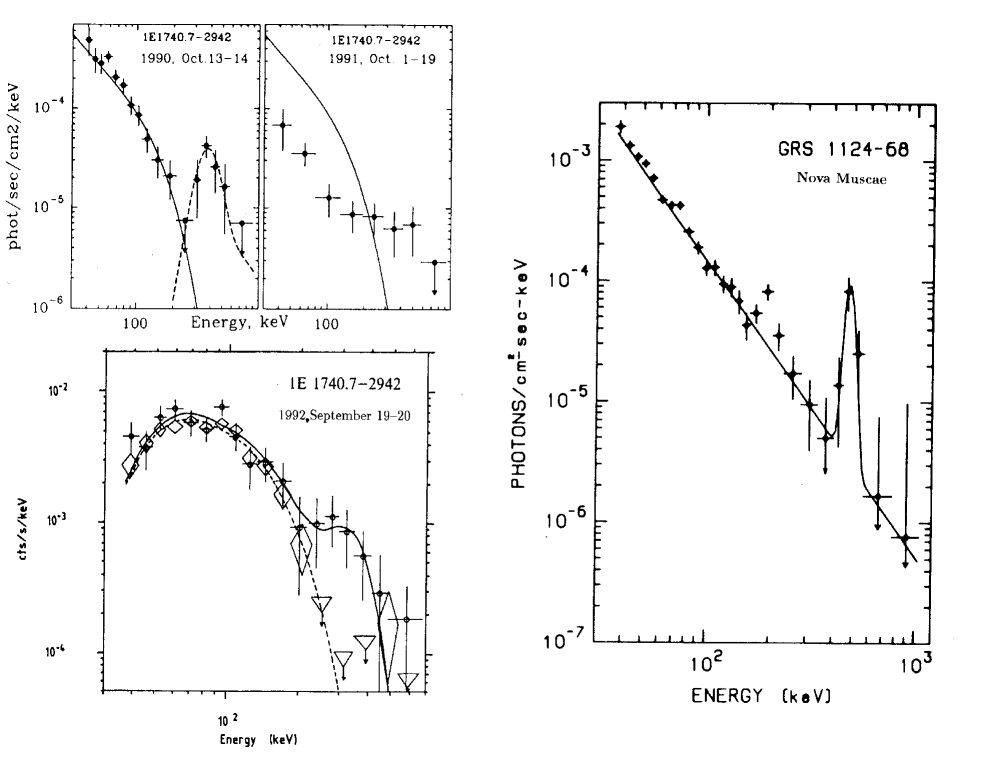
Fig. 6.: Energy spectra of the 1E source (Bouchet et al. 1991; Churazov et al. 1993, 1994; Cordier et al. 1993) and Nova Muscae (Goldwurm et al. 1992) observed by SIGMA are shown together with fits of the authors. For September 1992 flare shown is counts s^-1 keV^-1. The dashed line in the upper left panel shows the annihilation line shape for Gaussian-like injection, $\sim\exp[-(\gamma-4)^{2}]$, of energetic particles into the thermal plasma of $kT=35$ keV for $E/A=20$. The line is shifted left to approach the data.

The Galactic center region was intensively monitored by SIGMA telescope since 1990. Three times during these years a broad excess was observed in the 200–500 keV region (Fig.6).

In an observation performed between 1990 October 13 and 14, a spectacular unexpected feature was found in the 1E emission spectrum, the corresponding flux was estimated at $(0.9-1.3)\times 10^{-2}$ photons cm^-2 s^-1, with a line width of $180-240$ keV (Bouchet et al. 1991; Sunyaev et al. 1991). The observations of this region performed two days before (on October 10–11), and a few hours after (October 14–15) did not exhibit any spectral feature beyond 200 keV. The total duration of this state is estimated between 18 and about 70 hr.

Seven October 1991 observations have shown an evident excess at high energies, while the source was in a low state (Churazov et al. 1993). The excess was observed during 19 days and was not so intensive as in October 1990, the average flux was $(1.9\pm 0.6)\times 10^{-3}$ photons cm^-2 s^-1 in the 300–600 keV region.

The 1992 September 19–20 observational session (Sep. 19.42–20.58) showed a feature beyond 200 keV (Cordier et al. 1993), which resembles that of 1990 October 13–14. The line flux was estimated as $4.28_{-1.50}^{+2.70}\times 10^{-3}$ photons cm^-2 s^-1. The previous (Sep. 18.59–19.30) and the next (Sep. 22.57–23.14) sessions did not show any evidence for emission in excess of 200 keV, restricting the lifetime of the state between 27 and about 75 hr, while the rise time approaches probably several hours.

The spectral features observed by SIGMA are, commonly believed, related to electron-positron annihilation. Relatively small line widths imply that the temperature of the emitting region is quite low, $kT\approx 35-45$ keV for 1E and 4–5 keV for Nova Muscae. Since the hard X-ray spectra $<300$ keV showed no changes, most probably that electron-positron pairs produced somewhere close to the central object were injected into surrounding space where they cool and annihilate. Radiation pressure of a near-Eddington source alone can accelerate $e^{+}e^{-}$-plasma up to the bulk Lorentz factor of $\gamma_{0}\sim 2-5$ (Kovner 1984), while Comptonization by the emergent radiation field (Levich & Syunyaev 1971) could provide a mechanism for cooling the pairs which further annihilate “in flight” (for a discussion see also Gilfanov et al. [1991, 1994]). If there is enough matter around a source, then particles slow down due to Coulomb energy losses and annihilate in the medium. We explore further this last possibility by checking whether the inferred parameters of the emitting region are consistent with those obtained by other ways. We assume single and short particle ejection on a timescale of hours. It seems reasonable: since the ejection would probably impact on the whole spectrum, longer spectral changes would be observable.

Suggesting that the energetic particles slow down due to Coulomb scattering in the surrounding matter, one can estimate its (electron) number density

$$n_{-}\approx{\gamma_{0}-1\over\pi r_{e}^{2}c\,\Delta_{i}}\left({d\gamma\over dt}\right)^{-1},$$ (45)

where $\gamma_{0}$ is the initial Lorentz factor of the plasma stream, $c$ is the light speed, and $\Delta_{i}$ is the characteristic time scale of the annihilation line appearance. The Coulomb energy loss rate in a medium of $kT\leq 0.1$ is $(d\gamma/dt)\approx 70-100$ (see Fig.1). Taking a reasonable value for the bulk Lorentz factor, $\gamma_{0}\approx 3$ (e.g., Kovner 1984), one can obtain estimations of the order of magnitude as $n_{-}\approx 2.2\times 10^{7}$cm^-3$(\Delta_{i}/2$days$)^{-1}$ for the 1E source, and $n_{-}\approx 1.5\times 10^{8}$cm^-3$(\Delta_{i}/5$hr$)^{-1}$ for Nova Muscae.

If the energetic particles were injected into the medium only once, then the annihilation feature lifetime $\Delta_{d}$ is directly connected with annihilation rate as $\Delta_{d}^{-1}\approx\pi r_{e}^{2}c\,n_{-}A(\gamma)$. It yields one more estimation of the number density in the emitting region

$$n_{-}\approx{1\over\pi r_{e}^{2}c\,\Delta_{d}\,A(\gamma)}\approx 1.55\times 10^{9}{\rm\ cm}^{-3}\ \left({\Delta_{d}\over 1{\rm\ day}}\right)^{-1}.$$ (46)

Annihilation rate $A(\gamma)$ is a weak function of $\gamma$ (see Fig.1) and we can take it equal to a constant $A=A(1)\approx 1$. Total duration of the hard state is $\Delta_{d}\approx 18-70$ hr for the 1E source and $\Delta_{d}\leq 10$ days for Nova Muscae, that gives $n_{-}\approx(5-20)\times 10^{8}$ cm^-3 and $n_{-}\approx 1.5\times 10^{8}$cm^-3$(\Delta_{d}/10$days$)^{-1}$, correspondingly. The values obtained from eq.(45)–(46) restrict the electron number density in the volume where particles slow down and annihilate.

Being equated eq.(45)–(46) give an obvious relation between the time scales

$${\Delta_{d}\over\Delta_{i}}={1\over A(\gamma_{0}-1)}{d\gamma\over dt}.$$ (47)

Therefore, to be consistent with the annihilation lifetime the annihilation rise time for the 1E source should be $\Delta_{i}\approx 1-2$ hr. This is supported by the 1992 September 19–20 observation when the annihilation rise time was restricted by a few hours.

Table 1.: Observational data and parameters of the emitting region.

	1E 1740.7–2942
	1990 Oct. 13–14	1992 Sep. 19–20	Nova Muscae
Annihilation rise time, $\Delta_{i}$	$\mathrel{\mathchoice{\vbox{\offinterlineskip\halign{\hfil$\displaystyle#$\hfil\cr<\cr\sim\cr}}}{\vbox{\offinterlineskip\halign{\hfil$\textstyle#$\hfil\cr<\cr\sim\cr}}}{\vbox{\offinterlineskip\halign{\hfil$\scriptstyle#$\hfil\cr<\cr\sim\cr}}}{\vbox{\offinterlineskip\halign{\hfil$\scriptscriptstyle#$\hfil\cr<\cr\sim\cr}}}}2$ days (1–2 hr)∗	few hours	$\sim 5$ hr
Annihilation lifetime, $\Delta_{d}$	18–70 hr	27–75 hr	$\mathrel{\mathchoice{\vbox{\offinterlineskip\halign{\hfil$\displaystyle#$\hfil\cr<\cr\sim\cr}}}{\vbox{\offinterlineskip\halign{\hfil$\textstyle#$\hfil\cr<\cr\sim\cr}}}{\vbox{\offinterlineskip\halign{\hfil$\scriptstyle#$\hfil\cr<\cr\sim\cr}}}{\vbox{\offinterlineskip\halign{\hfil$\scriptscriptstyle#$\hfil\cr<\cr\sim\cr}}}}10$ days
Annihilation photon flux, $F_{500}$ (photons cm-2 s-1)	$10^{-2}$	$4.3\times 10^{-3}$	$6\times 10^{-3}$
Total line flux, $L_{500}$ (photons s-1)	$8.6\times 10^{43}$ (at 8.5 kpc)	$3.7\times 10^{43}$	$7.2\times 10^{41}$ (at 1 kpc)
Line width, $W$ (keV)	240	180	40
Plasma temperature, $kT_{e}$ (keV)	$35-45$		$3-4$
Column density, $N_{H}$ (cm-2)	$\sim 10^{23}$		$\sim 10^{21}$
Coulomb energy loss rate, $d\gamma/dt$	70		100
Annihilation rate, $A$	1		1
Electron number density, $n_{-}$ (cm-3)	$(5-20)\times 10^{8}$		$1.5\times 10^{8}$
Size of the emitting region, $\lambda$ (cm)	$(1.1-20)\times 10^{13}$		$(1.3-50)\times 10^{13}$

• Our estimation.

The size of the emitting region $\lambda$ could be estimated from a simple relation $n_{+}\lambda^{3}\sim\Delta_{d}L_{500}/2$ if we assume the upper limit for the positron number density $n_{+}\leq n_{-}$. It gives $\lambda\mathrel{\mathchoice{\vbox{\offinterlineskip\halign{\hfil$\displaystyle#$\hfil\cr>\cr\sim\cr}}}{\vbox{\offinterlineskip\halign{\hfil$\textstyle#$\hfil\cr>\cr\sim\cr}}}{\vbox{\offinterlineskip\halign{\hfil$\scriptstyle#$\hfil\cr>\cr\sim\cr}}}{\vbox{\offinterlineskip\halign{\hfil$\scriptscriptstyle#$\hfil\cr>\cr\sim\cr}}}}1.34\times 10^{13}$cm$(\Delta_{d}/1$day$)^{2/3}\approx(1.1-2.7)\times 10^{13}$ cm for 1E and $\lambda\mathrel{\mathchoice{\vbox{\offinterlineskip\halign{\hfil$\displaystyle#$\hfil\cr>\cr\sim\cr}}}{\vbox{\offinterlineskip\halign{\hfil$\textstyle#$\hfil\cr>\cr\sim\cr}}}{\vbox{\offinterlineskip\halign{\hfil$\scriptstyle#$\hfil\cr>\cr\sim\cr}}}{\vbox{\offinterlineskip\halign{\hfil$\scriptscriptstyle#$\hfil\cr>\cr\sim\cr}}}}1.3\times 10^{13}$cm$(\Delta_{d}/10$days$)^{2/3}$ for Nova Muscae, which are well inside of the upper limits $\lambda<c\Delta_{i}\approx 2.2\times 10^{14}$cm$(\Delta_{i}/2$hr$)$ and $\leq 5\times 10^{14}$ cm, correspondingly. From the above consideration follows that emitting regions in both sources are optically thin and do not affect the Comptonized spectra at $<300$ keV nor the annihilation line form. Experimental data and the estimated parameters are summarized in Table 1.

The column density of the medium where injected particles slow down and annihilate should exceed the value $N_{H}\sim\lambda n_{-}$, which follows from previous estimations for $\lambda$ and $n_{-}$, viz. $2.1\times 10^{22}$cm^-2$(\Delta_{d}/1$day$)^{-1/3}\mathrel{\mathchoice{\vbox{\offinterlineskip\halign{\hfil$\displaystyle#$\hfil\cr<\cr\sim\cr}}}{\vbox{\offinterlineskip\halign{\hfil$\textstyle#$\hfil\cr<\cr\sim\cr}}}{\vbox{\offinterlineskip\halign{\hfil$\scriptstyle#$\hfil\cr<\cr\sim\cr}}}{\vbox{\offinterlineskip\halign{\hfil$\scriptscriptstyle#$\hfil\cr<\cr\sim\cr}}}}N_{H}<c\Delta_{i}n_{-}\approx 1.1\times 10^{23}$cm^-2 for 1E, where we took into account eq.(47), and $N_{H}\mathrel{\mathchoice{\vbox{\offinterlineskip\halign{\hfil$\displaystyle#$\hfil\cr>\cr\sim\cr}}}{\vbox{\offinterlineskip\halign{\hfil$\textstyle#$\hfil\cr>\cr\sim\cr}}}{\vbox{\offinterlineskip\halign{\hfil$\scriptstyle#$\hfil\cr>\cr\sim\cr}}}{\vbox{\offinterlineskip\halign{\hfil$\scriptscriptstyle#$\hfil\cr>\cr\sim\cr}}}}2\times 10^{21}$cm^-2$(\Delta_{d}/10$days$)^{-1/3}$ for Nova Muscae. The total column density of the gas cloud measured along the line of sight, where the 1E source embedded, is high enough $N_{H}\approx 3\times 10^{23}$ cm^-2 (Bally & Leventhal 1991; Mirabel et al. 1991). Note that recent ASCA measurements of the column density to this source give a best fit value $N_{H}\approx 8\times 10^{22}$ cm^-2 (Sheth et al. 1996). For Nova Muscae the corresponding value is $N_{H}\sim 10^{21}$ cm^-2 (Greiner et al. 1991), less or marginally close to the obtained lower limit. If, on contrary, one suggests $n_{+}\ll n_{-}$ it yields a condition $N_{H}\gg 2\times 10^{21}$cm^-2$(\Delta_{d}/10$days$)^{-1/3}$, which considerably exceeds the measured value.

These estimations put us on to an idea that the 500 keV emission observed from Nova Muscae was coming from $e^{+}e^{-}$-plasma jet ($n_{+}\approx n_{-}$) rather than from particles injected in a gas cloud ($n_{+}\ll n_{-}$), therefore, particles have to annihilate “in flight” producing a relatively narrow line blue- or red-shifted dependently on the jet orientation. If so, then our estimation of the electron number density $n_{-}$ from annihilation time scale is related to the average electron/positron number density in the jet, its total volume is of $\lambda^{3}\sim 2\times 10^{39}$cm³$(\Delta_{d}/10$days$)^{2}$. The reported 6%–7% redshift of the line centroid (Goldwurm et al. 1992; Sunyaev et al. 1992) supports probably the annihilation-in-jet hypothesis, although authors noted that statistical significance of this shift is not very high. The large size of the emitting region and a small width of the line, both except the gravitational origin of the redshift, since in this case the annihilation region have to be quite close to the central object $\sim 10R_{g}$ where typical flow velocities should result in a much broader line (Gilfanov et al. 1991). The Compton scattering of the anisotropic emergent radiation could provide effective mechanism for blowing away and acceleration of $e^{+}e^{-}$-pair plasma (e.g., Kovner 1984; Misra & Melia 1993) cooling it at the same time. Since the maximal energy during the X-ray flare of Nova Muscae released near $\sim 1$keV (Greiner et al. 1991), the average kinetic energy per particle should be nearly the same (which is consistent with the small line width).

The case of the 1E source is not definitively clear, because our estimations give $n_{-}\mathrel{\mathchoice{\vbox{\offinterlineskip\halign{\hfil$\displaystyle#$\hfil\cr>\cr\sim\cr}}}{\vbox{\offinterlineskip\halign{\hfil$\textstyle#$\hfil\cr>\cr\sim\cr}}}{\vbox{\offinterlineskip\halign{\hfil$\scriptstyle#$\hfil\cr>\cr\sim\cr}}}{\vbox{\offinterlineskip\halign{\hfil$\scriptscriptstyle#$\hfil\cr>\cr\sim\cr}}}}n_{+}$ in the emitting region. Two flares, October 1990 and September 1992, have shown very similar time scales, spectra and photon fluxes, which are consistent with single injection of energetic particles into the thermal (hydrogen) plasma. Meanwhile, the redshift of the line $\sim 25$% reported by authors (Bouchet et al. 1991; Sunyaev et al. 1991; Cordier et al. 1993) implies that positrons probably annihilate in a plasma stream moving away from the observer. The estimation of the size of the emitting region ruled out its gravitational nature, since it is too large in comparison with gravitational radius of a stellar mass black hole. A natural explanation of this controversial picture is that the propagating plasma stream captures matter from the source environment and annihilation occurs in a moving plasma volume. In this case the estimation of the electron number density $n_{-}$ is related to the average electron number density in the jet, $\lambda^{3}\mathrel{\mathchoice{\vbox{\offinterlineskip\halign{\hfil$\displaystyle#$\hfil\cr>\cr\sim\cr}}}{\vbox{\offinterlineskip\halign{\hfil$\textstyle#$\hfil\cr>\cr\sim\cr}}}{\vbox{\offinterlineskip\halign{\hfil$\scriptstyle#$\hfil\cr>\cr\sim\cr}}}{\vbox{\offinterlineskip\halign{\hfil$\scriptscriptstyle#$\hfil\cr>\cr\sim\cr}}}}2.4\times 10^{39}$cm³$(\Delta_{d}/1$day$)^{2}$ gives its total volume, and the jet length has to be of the order of $\sim 0.2c\Delta_{d}\approx 5.2\times 10^{14}$cm$(\Delta_{d}/1$day$)$.

While a part of the $e^{+}e^{-}$-pair probably annihilate in a thermal plasma near the 1E source producing the broad line, the remainder could escape into a molecular cloud, which was found to be associated with the 1E source (Bally & Leventhal 1991; Mirabel et al. 1991). The time scale for slowing down due to the scattering could be obtained from eq.(45). Taking $\sim 10^{5}$ cm^-3 for the average number density of the molecular cloud near 1E (Bally & Leventhal 1991; Mirabel et al. 1991) one gets $\Delta_{i}\mathrel{\mathchoice{\vbox{\offinterlineskip\halign{\hfil$\displaystyle#$\hfil\cr<\cr\sim\cr}}}{\vbox{\offinterlineskip\halign{\hfil$\textstyle#$\hfil\cr<\cr\sim\cr}}}{\vbox{\offinterlineskip\halign{\hfil$\scriptstyle#$\hfil\cr<\cr\sim\cr}}}{\vbox{\offinterlineskip\halign{\hfil$\scriptscriptstyle#$\hfil\cr<\cr\sim\cr}}}}1$ year, the same as that obtained by Ramaty et al. (1992). The size of the turbulent region in the cloud caused by propagation of a dense jet should be of the same order. It agrees well with the length 2–4 ly (15–30 arcsec at the 8.5 kpc distance) of a double-sided radio jet from the 1E source found recently with the VLA (Mirabel et al. 1992).

If the lines from the 1E source (Fig.6) were produced by continuous injection of energetic particles, then the observations of the narrow 511 keV line emission from the Galactic center allows to put an upper limit on the particle escape rate into the interstellar medium. Recent reanalysis of HEAO 3 data has shown that under suggestion of a single point source at the Galactic center narrow line intensities are $F_{511}=(1.25\pm 0.18)\times 10^{-3}$ photons cm^-2 s^-1 for the fall of 1979 and $F_{511}=(0.99\pm 0.18)\times 10^{-3}$ photons cm^-2 s^-1 for the spring of 1980 (Mahoney et al. 1994). Taking $\tau_{0}=1$ yr for the positron lifetime in $10^{5}$ cm^-3 dense cold molecular cloud (Ramaty et al. 1992), and suggesting one hard state of $\Delta_{d}\mathrel{\mathchoice{\vbox{\offinterlineskip\halign{\hfil$\displaystyle#$\hfil\cr>\cr\sim\cr}}}{\vbox{\offinterlineskip\halign{\hfil$\textstyle#$\hfil\cr>\cr\sim\cr}}}{\vbox{\offinterlineskip\halign{\hfil$\scriptstyle#$\hfil\cr>\cr\sim\cr}}}{\vbox{\offinterlineskip\halign{\hfil$\scriptscriptstyle#$\hfil\cr>\cr\sim\cr}}}}2$ days long per period $\tau_{0}$, one can obtain an escape rate $E/A\approx{F_{511}\,\tau_{0}\over F_{500}\,\Delta_{d}}\mathrel{\mathchoice{\vbox{\offinterlineskip\halign{\hfil$\displaystyle#$\hfil\cr<\cr\sim\cr}}}{\vbox{\offinterlineskip\halign{\hfil$\textstyle#$\hfil\cr<\cr\sim\cr}}}{\vbox{\offinterlineskip\halign{\hfil$\scriptstyle#$\hfil\cr<\cr\sim\cr}}}{\vbox{\offinterlineskip\halign{\hfil$\scriptscriptstyle#$\hfil\cr<\cr\sim\cr}}}}20$, where we took $F_{500}=10^{-2}$ photons cm^-2 s^-1 (see Table 1). This is consistent with the upper limits of 1990 October 13–14 spectrum and the two most energetic points in 1992 September 19–20 spectrum. The dashed line in 1990 October 13–14 spectrum (Fig.6) shows the annihilation line shape for Gaussian-like injection, $\sim\exp[-(\gamma-4)^{2}]$, of energetic particles into the thermal plasma of $kT=35$ keV for $E/A=20$. The longest hard state ($\sim 19$ days) with the average flux of $F_{500}\approx 2\times 10^{-3}$ photons cm^-2 s^-1 observed in October 1991 places the upper limit at almost the same level $E/A\approx 10$.

10 Conclusion

We have presented the accurate formulas in the form of a simple expression or an one-fold integral for the energy losses and gains of particles scattered by a Maxwell-Boltzmann plasma. The processes concerned are the Coulomb scattering, $e^{+}e^{-}$-, $ee$- and $ep$-bremsstrahlung as well as Comptonization in the Klein-Nishina regime.

The problem of positron propagation is treated in a Fokker-Planck approach, which can be easily generalized to include inelastic processes, stochastic acceleration etc. We have shown that the escape of positrons in the form of pair plasma has an effect on the positron distribution causing, in some cases, a strong deviation from a Maxwellian. When the energy of injected particles essentially exceeds the average one of plasma particles, the deviation appears as a deficit at lower energies and an extended tail of the distribution that leads to a widening and smoothing of the annihilation feature in the spectrum. In the case where the energy of particles injected is close to the average energy of plasma particles, the deviation appears as an injection bump and a deficit in the tail of the distribution. Meanwhile, it does not lead to visible distortions of the annihilation line shape which is similar to that of thermal plasmas.

The performed calculations allow us to obtain reliable estimations of the electron number density and the size of the emitting regions in Nova Muscae and the 1E1740.7–2942 source, suggesting that spectral features in 300–600 keV region observed by SIGMA telescope are due to the electron-positron annihilation in thermal plasma. We conclude that in the case of Nova Muscae the observed radiation is coming from a pair plasma jet, $n_{+}\approx n_{-}$, rather than from a gas cloud. The case of 1E1740.7–2942 is not definitively clear, $n_{+}\mathrel{\mathchoice{\vbox{\offinterlineskip\halign{\hfil$\displaystyle#$\hfil\cr<\cr\sim\cr}}}{\vbox{\offinterlineskip\halign{\hfil$\textstyle#$\hfil\cr<\cr\sim\cr}}}{\vbox{\offinterlineskip\halign{\hfil$\scriptstyle#$\hfil\cr<\cr\sim\cr}}}{\vbox{\offinterlineskip\halign{\hfil$\scriptscriptstyle#$\hfil\cr<\cr\sim\cr}}}}n_{-}$. Although the observational data are consistent with annihilation in (hydrogen) plasma at rest, the redshift of the line suggests that it could be also a stream of pair plasma with matter captured from the source environment.

• The authors thank Anatoly Tur for helpful discussions, useful comments of an anonymous referee are greatly acknowledged. I.M. is grateful to the SIGMA team of CESR for warm hospitality and facilities which made his stay in Toulouse very fruitful and pleasant. This work was partly supported through a post-doctoral fellowship of the French Ministry of Research.

References

• 1 Bally J., Leventhal M., 1991, Nature 353, 234
• 2 Bouchet L., et al., 1991, ApJ 383, L45
• 3 Churazov E., et al., 1993, ApJ 407, 752
• 4 Churazov E., et al., 1994, ApJS 92, 381
• 5 Cordier B., et al., 1993, A&A 275, L1
• 6 Dermer C. D., 1984, ApJ, 280, 328
• 7 Dermer C. D., 1985, ApJ, 295, 28
• 8 Dermer C. D., Liang E. P., 1989, ApJ 339, 512
• 9 Gilfanov M., et al., 1991, Soviet Astron. Lett. 17, 437
• 10 Gilfanov M., et al., 1994, ApJS 92, 411
• 11 Goldwurm A., et al., 1992, ApJ 389, L79
• 12 Gould R. J., 1981, Phys. Fluids, 24, 102
• 13 Greiner J., et al., 1991, in Proc. Workshop on Nova Muscae, ed. S. Brandt, Danish Space Research Inst., Lyngby, p.79
• 14 Guessoum N., Ramaty R., Lingenfelter R. E., 1991, ApJ 378, 170
• 15 Haug E., 1975, Z. Naturforsch. 30a, 1546
• 16 Haug E., 1985a, Phys. Rev. D31, 2120
• 17 Haug E., 1985b, Phys. Rev. D32, 1594
• 18 Haug E., 1985c, A&A 148, 386
• 19 Jauch J. M., Rohrlich F., 1976, The Theory of Photons and Electrons, Springer-Verlag, Berlin
• 20 Jones F. C., 1965, Phys. Rev. 137, B1306
• 21 Kovner I., 1984, A&A 141, 341
• 22 Leventhal M., MacCallum C. J., Stang P. D., 1978, ApJ 225, L11
• 23 Levich E. V., Syunyaev R. A., 1971, Soviet Astron., 15, 363
• 24 Lifshitz E. M., Pitaevskii L. P., 1979, Physical Kinetics, Nauka, Moscow
• 25 Mahoney W. A., Ling J. C., Wheaton Wm. A., 1994, ApJS 92, 387
• 26 Mazets E. P., et al., 1982, Ap&SS 84, 173
• 27 Meirelles C. F., Liang E. P., 1993, in AIP 304, 2nd Compton Symp., eds. C.E. Fichtel, N. Gehrels, J.P. Norris, p.299
• 28 Mirabel I. F., et al., 1991, A&A 251, L43
• 29 Mirabel I. F., et al., 1992, Nature 358, 215
• 30 Misra R., Melia F., 1993, ApJ 419, L25
• 31 Moskalenko I. V., 1995, Proc. 24th ICRC (Roma), 3, 794
• 32 Murphy R., et al., 1990, ApJ 358, 290
• 33 Parlier F., et al., 1990, in AIP 232, Gamma Ray Line Astrophysics, eds. P. Durouchoux, N. Prantzos, p.335
• 34 Ramaty R., Mészáros P., 1981, ApJ, 250, 384
• 35 Ramaty R., et al., 1992, ApJ 392, L63
• 36 Sheth S., et al., 1996, ApJ 468, 755
• 37 Stickforth J., 1961, Z. Physik 164, 1
• 38 Sunyaev R. A., Titarchuk L. G., 1980, A&A 86, 121
• 39 Sunyaev R. A., et al., 1991, ApJ 383, L49
• 40 Sunyaev R. A., et al., 1992, ApJ 389, L75
• 41 Svensson R., 1982, ApJ 258, 321
• 42 Svensson R., 1990, in Physical Processes in Hot Cosmic Plasmas, eds. W. Brinkmann, A.C. Fabian, F. Giovannelli, Kluwer, Dordrecht, p.357