SOLAR NEUTRINOS: WHERE WE ARE

Abstract

This talk compares standard model predictions for solar neutrino experiments with the results of actual observations. Here ‘standard model’ means the combined standard model of minimal electroweak theory plus a standard solar model. I emphasize the importance of recent analyses in which the neutrino fluxes are treated as free parameters, independent of any constraints from solar models, and the stunning agreement between the predictions of standard solar models and helioseismological measurements.

1 Introduction

Joe Taylor mentioned in his beautiful preceding review of pulsar phenomena that the discussion of pulsars has a long history at the Texas conferences. I want to add a footnote to his historical remarks: the subject of solar neutrinos has an even longer history in this context. Both Ray Davis and I gave invited talks [1, 2] on solar neutrinos at the 2nd Texas Conference, which was held in Austin, Texas in December 1964.

Solar neutrino research has now achieved the primary goal that was discussed in the 1964 Texas Conference, namely, the detection of solar neutrinos. This detection establishes empirically that the sun shines by fusing light nuclei in its interior.

The subject of solar neutrinos is entering a new phase in which large electronic detectors will yield vast amounts of diagnostic data. These new experiments [3, 4, 5], which will be described by Professor Totsuka in the following talk, will test the prediction of the minimal standard electroweak theory [6, 7, 8] that essentially nothing happens to electron type neutrinos after they are created by nuclear fusion reactions in the interior of the sun.

The four pioneering experiments—chlorine [9, 10] Kamiokande [11] GALLEX [12] and SAGE [13]—have all observed neutrino fluxes with intensities that are within a factors of a few of those predicted by standard solar models. Three of the experiments (chlorine, GALLEX, and SAGE) are radiochemical and each radiochemical experiment measures one number, the total rate at which neutrinos above a fixed energy threshold (which depends upon the detector) are captured. The sole electronic (non-radiochemical) detector among the initial experiments, Kamiokande, has shown that the neutrinos come from the sun, by measuring the recoil directions of the electrons scattered by solar neutrinos. Kamiokande has also demonstrated that the observed neutrino energies are consistent with the range of energies expected on the basis of the standard solar model.

Despite continual refinement of solar model calculations of neutrino fluxes over the past 35 years (see, e.g., the collection of articles reprinted in the book edited by Bahcall, Davis, Parker, Smirnov, and Ulrich [14]), the discrepancies between observations and calculations have gotten worse with time. All four of the pioneering solar neutrino experiments yield event rates that are significantly less than predicted by standard solar models.

This talk is organized as follows. I first discuss in section 2 the three solar neutrino problems. Then I review in section 3 the recent work by Heeger and Robinson [15] which treats the neutrino fluxes as free parameters and shows that the solar neutrino problems cannot be resolved within the context of minimal standard electroweak theory unless solar neutrino experiments are incorrect. Next I discuss in section 4 the stunning agreement between the values of the sound velocity calculated from standard solar models and the values obtained from helioseismological measurements. Finally, in section 5 I compare the success of the MSW neutrino mixing hypothesis with the success of the solar ³He mixing hypothesis recently discussed by Cumming and Haxton[16].

See http://www.sns.ias.edu/${\scriptstyle\sim}$jnb for further information about solar neutrinos, including viewgraphs, preprints, and numerical data.

2 Three Solar Neutrino Problems

I will first compare the predictions of the combined standard model with the results of the operating solar neutrino experiments. By ‘combined’ standard model, I mean the predictions of the standard solar model and the predictions of the minimal electroweak theory. We need a solar model to tell us how many neutrinos of what energy are produced in the sun and we need electroweak theory to tell us how the number and flavor content of the neutrinos are changed as they make their way from the center of the sun to detectors on earth.

We will see that this comparison leads to three different discrepancies between the calculations and the observations, which I will refer to as the three solar neutrino problems.

Figure 1 shows the measured and the calculated event rates in the four ongoing solar neutrino experiments. This figure reveals three discrepancies between the experimental results and the expectations based upon the combined standard model. As we shall see, only the first of these discrepancies depends sensitively upon predictions of the standard solar model.

2.1 Calculated versus Observed Absolute Rate

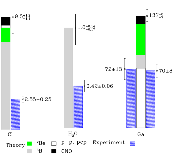
Figure 1: Comparison of measured rates and standard-model predictions for four solar neutrino experiments.

The first solar neutrino experiment to be performed was the chlorine radiochemical experiment, which detects electron-type neutrinos that are more energetic than $0.81$ MeV. After more than 25 years of the operation of this experiment, the measured event rate is $2.55\pm 0.25$ SNU, which is a factor $\sim 3.6$ less than is predicted by the most detailed theoretical calculations, $9.5_{-1.4}^{+1.2}$ SNU [17, 18]. A SNU is a convenient unit to describe the measured rates of solar neutrino experiments: $10^{-36}$ interactions per target atom per second. Most of the predicted rate in the chlorine experiment is from the rare, high-energy ⁸B neutrinos, although the ⁷Be neutrinos are also expected to contribute significantly. According to standard model calculations, the $pep$ neutrinos and the CNO neutrinos (for simplicity not discussed here) are expected to contribute less than 1 SNU to the total event rate.

This discrepancy between the calculations and the observations for the chlorine experiment was, for more than two decades, the only solar neutrino problem. I shall refer to the chlorine disagreement as the “first” solar neutrino problem.

2.2 Incompatibility of Chlorine and Water (Kamiokande) Experiments

The second solar neutrino problem results from a comparison of the measured event rates in the chlorine experiment and in the Japanese pure-water experiment, Kamiokande. The water experiment detects higher-energy neutrinos, those with energies above $7$ MeV, by neutrino-electron scattering: $\nu~{}+~{}e~{}\longrightarrow\nu^{\prime}~{}+~{}e^{\prime}.$ According to the standard solar model, ⁸B beta decay is the only important source of these higher-energy neutrinos.

The Kamiokande experiment shows that the observed neutrinos come from the sun. The electrons that are scattered by the incoming neutrinos recoil predominantly in the direction of the sun-earth vector; the relativistic electrons are observed by the Cherenkov radiation they produce in the water detector.

In addition, the Kamiokande experiment measures the energies of individual scattered electrons and therefore provides information about the energy spectrum of the incident solar neutrinos. The observed spectrum of electron recoil energies is consistent with that expected from ⁸B neutrinos. However, small angle scattering of the recoil electrons in the water prevents the angular distribution from being determined well on an event-by-event basis, which limits the constraints the experiment places on the incoming neutrino energy spectrum.

The event rate in the Kamiokande experiment is determined by the same high-energy ⁸B neutrinos that are expected, on the basis of the combined standard model, to dominate the event rate in the chlorine experiment. I have shown[19] that solar physics changes the shape of the ⁸B neutrino spectrum by less than 1 part in $10^{5}$ . Therefore, we can calculate the rate in the chlorine experiment that is produced by the ⁸B neutrinos observed in the Kamiokande experiment (above 7 MeV). This partial (⁸B) rate in the chlorine experiment is $3.2\pm 0.45$ SNU, which exceeds the total observed chlorine rate of $2.55\pm 0.25$ SNU.

Comparing the rates of the Kamiokande and the chlorine experiments, one finds that the net contribution to the chlorine experiment from the $pep$, ⁷Be, and CNO neutrino sources is negative: $-0.66\pm 0.52$ SNU. The standard model calculated rate from $pep$, ⁷Be, and CNO neutrinos is 1.9 SNU. The apparent incompatibility of the chlorine and the Kamiokande experiments is the “second” solar neutrino problem. The inference that is often made from this comparison is that the energy spectrum of ${\rm{}^{8}B}$ neutrinos is changed from the standard shape by physics not included in the simplest version of the standard electroweak model.

2.3 Gallium Experiments: No Room for ⁷Be Neutrinos

The results of the gallium experiments, GALLEX and SAGE, constitute the third solar neutrino problem. The average observed rate in these two experiments is $70.5\pm 7$ SNU, which is fully accounted for in the standard model by the theoretical rate of $73$ SNU that is calculated to come from the basic $p$-$p$ and $pep$ neutrinos (with only a 1% uncertainty in the standard solar model $p$-$p$ flux). The ⁸B neutrinos, which are observed above $7.5$ MeV in the Kamiokande experiment, must also contribute to the gallium event rate. Using the standard shape for the spectrum of ${\rm{}^{8}B}$ neutrinos and normalizing to the rate observed in Kamiokande, ${\rm{}^{8}B}$ contributes another $7$ SNU, unless something happens to the lower-energy neutrinos after they are created in the sun. (The predicted contribution is 16 SNU on the basis of the standard model.) Given the measured rates in the gallium experiments, there is no room for the additional $34\pm 4$ SNU that is expected from ⁷Be neutrinos on the basis of standard solar models.

The seeming exclusion of everything but $p$-$p$ neutrinos in the gallium experiments is the “third” solar neutrino problem. This problem is essentially independent of the previously-discussed solar neutrino problems, since it depends strongly upon the $p$-$p$ neutrinos that are not observed in the other experiments and whose calculated flux is approximately model-independent.

The missing ⁷Be neutrinos cannot be explained away by any change in solar physics. The ⁸B neutrinos that are observed in the Kamiokande experiment are produced in competition with the missing ⁷Be neutrinos; the competition is between electron capture on ⁷Be versus proton capture on ⁷Be. Solar model explanations that reduce the predicted ${\rm{}^{7}Be}$ flux generically reduce much more (too much) the predictions for the observed ${\rm{}^{8}B}$ flux.

The flux of ⁷Be neutrinos, $\phi({\rm{}^{7}Be})$, is independent of measurement uncertainties in the cross section for the nuclear reaction ${\rm{}^{7}Be}(p,\gamma)^{8}$B; the cross section for this proton-capture reaction is the most uncertain quantity that enters in an important way in the solar model calculations. The flux of ⁷Be neutrinos depends upon the proton-capture reaction only through the ratio

$$\phi({\rm{}^{7}Be})~{}\propto~{}{{R(e)}\over{R(e)+R(p)}},$$ (1)

where $R(e)$ is the rate of electron capture by ⁷Be nuclei and $R(p)$ is the rate of proton capture by ⁷Be. With standard parameters, solar models yield $R(p)\approx 10^{-3}R(e)$. Therefore, one would have to increase the value of the ${\rm{}^{7}Be}(p,\gamma)^{8}$B cross section by more than 2 orders of magnitude over the current best-estimate (which has an estimated uncertainty of $\sim$ 10%) in order to affect significantly the calculated ⁷Be solar neutrino flux. The required change in the nuclear physics cross section would also increase the predicted neutrino event rate by more than 100 in the Kamiokande experiment, making that prediction completely inconsistent with what is observed. (From time to time, papers have been published claiming to solve the solar neutrino problem by artificially changing the rate of the ⁷Be electron capture reaction. Equation (1) shows that the flux of ⁷Be neutrinos is actually independent of the rate of the electron capture reaction to an accuracy of better than 1%.)

I conclude that either: 1) at least three of the four operating solar neutrino experiments (the two gallium experiments plus either chlorine or Kamiokande) have yielded misleading results, or 2) physics beyond the standard electroweak model is required to change the neutrino energy spectrum (or flavor content) after the neutrinos are produced in the center of the sun.

3 “The Last Hope”: No Solar Model

The clearest way to see that the results of the four solar neutrino experiments are inconsistent with the predictions of the minimal electroweak model is not to use standard solar models at all in the comparison with observations. This is what Berezinsky, Fiorentini, and Lissia [20] have termed “The Last Hope” for a solution of the solar neutrino problems without introducing new physics.

Let me now explain how model independent tests are made.

Let $\phi_{i}(E)$ be the normalized shape of the neutrino energy spectrum from one of the $i$ neutrino sources in the sun (e.g., ⁸B or $p-p$ neutrinos). I have shown [19] that the shape of the neutrino energy spectra that result from radioactive decays, ⁸B, ¹³N, ¹⁵O, and ¹⁷F, are the same to $1$ part in $10^{5}$ as the laboratory shapes. The $p-p$ neutrino energy spectrum, which is produced by fusion has a slight dependence on the solar temperature, which affects the shape by about $1$%. The energies of the neutrino lines from ⁷Be and $pep$ electron capture reactions are also only slightly shifted, by about $1$% or less, because of the thermal energies of particles in the solar core.

Thus one can test the hypothesis that an arbitrary linear combination of the normalized neutrino spectra,

$$\Phi(E)~{}=~{}\sum_{i}\alpha_{i}\phi_{i}(E),$$ (2)

can fit the results of the neutrino experiments. One can add a constraint to Eq. (2) that embodies the fact that the sun shines by nuclear fusion reactions that also produce the neutrinos. The explicit form of this luminosity constraint is

$$\frac{L_{\odot}}{4\pi r^{2}}=\sum_{j}\beta_{j}\phi_{j}~{},$$ (3)

where the eight coefficients, $\beta_{j}$, are given in Table VI of the paper by Bahcall and Krastev [21].

The first demonstration that the four pioneering experiments are by themselves inconsistent with the assumption that nothing happens to solar neutrinos after they are created in the core of the sun was by Hata, Bludman, and Langacker [22]. They showed that the solar neutrino data available by late 1993 were incompatible with any solution of equations (2) and (3) at the 97% C.L.

In the most recent and complete analysis in which the neutrino fluxes are treated as free parameters, Heeger and Robertson [15] showed that the data presented at the Neutrino ’96 Conference in Helsinki are inconsistent with equations (2) and (3) at the 99.5% C.L. Even if they omitted the luminosity constraint, equation (3), they found inconsistency at the 94% C.L.

It seems to me that these demonstrations are so powerful and general that there is very little point in discussing potential “solutions” to the solar neutrino problem based upon hypothesized non-standard scenarios for solar models.

4 Comparison with Helioseismological Measurements

Helioseismology has recently sharpened the disagreement between observations and the predictions of solar models with standard (non-oscillating) neutrinos. This development has occurred in two ways.

Helioseismology has confirmed the correctness of including diffusion in the solar models and the effect of diffusion leads to somewhat higher predicted events in the chlorine and Kamiokande solar neutrino experiments [17]. Even more importantly, helioseismology has demonstrated that the sound velocities predicted by standard solar models agree with extraordinary precision with the sound velocities of the sun inferred from helioseismological measurements [18]. Because of the precision of this agreement, I am convinced that standard solar models cannot be in error by enough to make a major difference in the solar neutrino problems.

The physical basis for the helioseismological measurements was described beautifully by Jøergen Christensen-Dalsgaard in his talk yesterday afternoon. I recommend the text of his discussion that you will also find in these proceedings. You will see in Jøergen’s article references to other papers about helioseismology that you can use to become better acquainted with the subject.

I will report here on some comparisons that Marc Pinsonneault, Sarbani Basu, Jøergen, and I have done recently which demonstrate the precise agreement between the sound velocities in standard solar models and the sound velocities inferred from helioseismological measurements. These results are based upon an article that has since appeared in Physical Review Letters [18].

Since the deep solar interior behaves essentially as a fully ionized perfect gas, $c^{2}\propto T/\mu$ where $T$ is temperature and $\mu$ is mean molecular weight. The sound velocities in the sun are determined from helioseismology to a very high accuracy, better than $0.2$% rms throughout nearly all the sun. Thus even tiny fractional errors in the model values of $T$ or $\mu$ would produce measurable discrepancies in the precisely determined helioseismological sound speed

$${\delta c\over c}\simeq{1\over 2}\left({\delta T\over T}-{\delta\mu\over\mu}\right)\;.$$ (4)

The remarkable numerical agreement between standard predictions and helioseismological observations, which I will discuss in the following remarks, rules out solar models with temperature or mean molecular weight profiles that differ significantly from standard profiles. The helioseismological data essentially rule out solar models in which deep mixing has occurred (cf. PRL paper[23]) and argue against unmixed models in which the subtle effect of particle diffusion–selective sinking of heavier species in the sun’s gravitational field–is not included.

Figure 2 compares the sound speeds computed from three different solar models with the values inferred [24, 25] from the helioseismological measurements. The 1995 standard model of Bahcall and Pinsonneault (BP) [17], which includes helium and heavy element diffusion, is represented by the dotted line; the corresponding BP model without diffusion is represented by the dashed line. The dark line represents the best solar model which includes recent improvements [26, 27] in the OPAL equation of state and opacities, as well as helium and heavy element diffusion. For the OPAL EOS model, the rms discrepancy between predicted and measured sound speeds is $0.1$% (which may be due partly to systematic uncertainties in the data analysis).

Figure 2: Comparison of sound speeds predicted by different standard solar models with the sound speeds measured by helioseismology. There are no free parameters in the models; the microphysics is successively improved by first including diffusion and then by using a more comprehensive equation of state. The figure shows the fractional difference, $\delta c/c$, between the predicted model sound speed and the measured [24, 25] solar values as a function of radial position in the sun ($R_{\odot}$ is the solar radius). The dashed line refers to a model [17] in which diffusion is neglected and the dotted line was computed from a model [17] in which helium and heavy element diffusion are included. The dark line represents a model which includes recent improvements in the OPAL equation of state and opacities [26, 27].

In the outer parts of the sun, in the convective region between $0.7R_{\odot}$ to $0.95R_{\odot}$ (where the measurements end), the No Diffusion and the 1995 Diffusion model have discrepancies as large as $0.5$% (see Figure 2). The model with the Livermore equation of state [27], OPAL EOS, fits the observations remarkably well in this region. We conclude, in agreement with the work of other authors [28], that the OPAL (Livermore National Laboratory) equation of state provides a significant improvement in the description of the outer regions of the sun.

The agreement between standard models and solar observations is independent of the finer details of the solar model. The standard model of Christensen-Dalsgaard et al. [29], which is derived from an independent computer code with different descriptions of the microphysics, predicts solar sound speeds that agree everywhere with the measured speeds to better than $0.2$%.

Figure 2 shows that the discrepancies with the No Diffusion model are as large as $1$%. The mean squared discrepancy for the No Diffusion model is 22 times larger than for the best model with diffusion, OPAL EOS. If one supposed optimistically that the No Diffusion model were correct, one would have to explain why the diffusion model fits the data so much better. On the basis of Figure 2, we conclude that otherwise standard solar models that do not include diffusion, such as the model of Turck-Chièze and Lopez [30], are inconsistent with helioseismological observations. This conclusion is consistent with earlier inferences based upon comparisons with less complete helioseismological data [24, 31, 23], including the fact that the present-day surface helium abundance in a standard solar model agrees with observations only if diffusion is included [17].

Equation 4 and Figure 2 imply that any changes $\delta T/T$ from the standard model values of temperature must be almost exactly canceled by changes $\delta\mu/\mu$ in mean molecular weight. In the standard model, $T$ and $\mu$ vary, respectively, by a factor of $53$ and $43$% over the entire range for which $c$ has been measured and by $1.9$ and $39$% over the energy producing region. It would be a remarkable coincidence if nature chose $T$ and $\mu$ profiles that individually differ markedly from the standard model but have the same ratio $T/\mu$. Thus we expect that the fractional differences between the solar and the model temperature, $\delta T/T$, or mean molecular weights, $\delta\mu/\mu$, are of similar magnitude to $\delta c^{2}/c^{2}$, i.e. (using the larger rms error, $0.002$, for the solar interior),

$$|\delta T/T|,~{}|\delta\mu/\mu|~{}\mathrel{\raise 1.29167pt\hbox{$<$}\mkern-14.0mu\lower 2.58334pt\hbox{$\sim$}}~{}0.004.$$ (5)

How significant for solar neutrino studies is the agreement between observation and prediction that is shown in Figure 2? The calculated neutrino fluxes depend upon the central temperature of the solar model approximately as a power of the temperature, ${\rm Flux}\propto T^{n}$, where for standard models the exponent $n$ varies from $n\sim-1.1$ for the $p-p$ neutrinos to $n\sim+24$ for the ⁸B neutrinos [32]. Similar temperature scalings are found for non-standard solar models [33]. Thus, maximum temperature differences of $\sim 0.2\%$ would produce changes in the different neutrino fluxes of several percent or less, much less than required [34] to ameliorate the solar neutrino problems.

Figure 3 shows that the “mixed” model of Cummings and Haxton (CH) [16] (illustrated in their Figure 1) is grossly inconsistent with the observed helioseismological measurements. The vertical scale of Figure 3 had to be expanded by a factor of $2.5$ relative to Figure 2 in order to display the large discrepancies with observations for the mixed model. The discrepancies for the CH mixed model (dashed line in Figure 3) range from $+8$% to $-5$%. Since $\mu$ in a standard solar model decreases monotonically outward from the solar interior, the mixed model–with a constant value of $\mu$– predicts too large values for the sound speed in the inner mixed region and too small values in the outer mixed region. The asymmetric form of the discrepancies for the CH model is due to the competition between the assumed constant rescaling of the temperature in the BP No Diffusion model and the assumed mixing of the solar core (constant value of $\mu$). We also show in Figure 3 the relatively tiny discrepancies found for the new standard model, OPAL EOS.

Figure 3: Non-standard solar models compared with helioseismology. This figure is similar to Figure 2 except that the vertical scale is expanded. The dashed curve represents the sound speeds computed for the mixed solar model of Cumming and Haxton [16] with ³He mixing. The dotted line represents the sound speed for a solar model computed with the rate of the ${}^{3}{\rm He}(\alpha,\gamma)^{7}$Be reaction set equal to zero. For comparison, we also include the results for the new standard model labeled OPAL EOS in Figure 2.

More generally, helioseismology rules out all solar models with large amounts of interior mixing, unless finely-tuned compensating changes in the temperature are made. The mean molecular weight in the standard solar model with diffusion varies monotonically from $0.86$ in the deep interior to $0.62$ at the outer region of nuclear fusion ($R=0.25R\odot$) to $0.60$ near the solar surface. Any mixing model will cause $\mu$ to be constant and equal to the average value in the mixed region. At the very least, the region in which nuclear fusion occurs must be mixed in order to affect significantly the calculated neutrino fluxes [35, 36, 37, 38, 39]. Unless almost precisely canceling temperature changes are assumed, solar models in which the nuclear burning region is mixed ($R\mathrel{\raise 1.29167pt\hbox{$<$}\mkern-14.0mu\lower 2.58334pt\hbox{$\sim$}}0.25R_{\odot}$) will give maximum differences, $\delta c$, between the mixed and the standard model predictions, and hence between the mixed model predictions and the observations, of order

$${\delta c\over c}~{}=~{}{1\over 2}\left({{\mu-<\mu>}\over{\mu}}\right)~{}\sim~{}7\%~{}{\rm to}~{}10\%,$$ (6)

which is inconsistent with Figure 2.

Are the helioseismological measurements sensitive to the rates of the nuclear fusion reactions? In order to answer this question in its most extreme form, we have computed a model in which the cross section factor, $S_{34}$, for the ${}^{3}{\rm He}(\alpha,\gamma)^{7}{\rm Be}$ reaction is artificially set equal to zero. The neutrino fluxes computed from this unrealistic model have been used [35] to set a lower limit on the allowed rate of solar neutrinos in the gallium experiments if the solar luminosity is currently powered by nuclear fusion reactions. Figure 3 shows that although the maximum discrepancies ($\sim 1$%) for the $S_{34}=0$ model are much smaller than for mixed models, they are still large compared to the differences between the standard model and helioseismological measurements. The mean squared discrepancy for the $S_{34}=0$ model is 19 times larger than for the standard OPAL EOS model. We conclude that the $S_{34}=0$ model is not compatible with helioseismological observations.

To me, these results suggest strongly that the assumption on which they are based—nothing happens to the neutrinos after they are created in the interior of the sun—is incorrect.

5 ³He Mixing versus MSW Mixing

It is instructive to compare the success of the hypothesis of ³He solar mixing[16] with the success of the hypothesis of MSW neutrino mixing. I do so below.

$\bullet$Consistency With Solar Neutrino Experiments. The ³He mixing hypothesis is inconsistent at the 99.5% C.L. with solar neutrino experiments (a special case of the general result of Heeger and Robinson[15]); MSW mixing is consistent with the solar neutrino experiments (best value of $\chi^{2}$ is less than one per degree of freedom).

$\bullet$Consistency With Helioseismology. The ³He mixing hypothesis is inconsistent with helioseismology; mixing of the solar core necessarily implies $\sim 7$% discrepancies with the measured solar sound velocities. The standard solar model with no free parameters predicts sound velocities that agree with the measured velocities to a rms accuracy of 0.2% in the solar core.

$\bullet$Free Parameters. The ³He mixing has 3 free parameters; the MSW mixing has 2 free parameters.

6 Discussion

The combined predictions of the standard solar model and the standard electroweak theory disagree with the results of the four pioneering solar neutrino experiments. The disagreement persists even if the neutrino fluxes are treated as free parameters, without reference to any solar model.

The solar model calculations are in excellent agreement with helioseismological measurements of the sound velocity, providing further support for the inference that something happens to the solar neutrinos after they are created in the center of the sun.

Looking back on what was envisioned in 1964, I am astonished and pleased with what has been accomplished. In 1964, it was not clear that solar neutrinos could be detected. Now, they have been observed in different experiments and the theory of stellar energy generation by nuclear fusion has been directly confirmed. Moreover, particle theorists have shown that solar neutrinos can be used to study neutrino properties, a possibility that we did not even consider in 1964. In fact, much of the interest in the subject stems from the fact that the four pioneering experiments suggest that new neutrino physics may be revealed by solar neutrino measurements. Finally, helioseismology has confirmed to high precision predictions of the standard solar model, a possibility that also was not imagined in 1964.

References

References

- [1] John N. Bahcall, Proceedings of the 2nd Texas Symposium on Relativistic Astrophysics, December 1964, in Quasars and High-Energy Astronomy, eds. K.N. Douglas, E.L. Schucking, I. Robinson, J.A. Wheeler, A. Schild, and N.J. Woolf (Gordon and Breach, 1969) p. 321.
- [2] R. Davis, Jr., D.S. Harmer, and F.H. Nelly, Proceedings of the 2nd Texas Symposium on Relativistic Astrophysics, December 1964, in Quasars and High-Energy Astronomy, eds. K.N. Douglas, E.L. Schucking, I. Robinson, J.A. Wheeler, A. Schild, and N.J. Woolf (Gordon and Breach, 1969) p. 287.
- [3] C. Arpesella et al., BOREXINO proposal, Vols. 1 and 2, eds. G. Bellini, R. Raghavan, et al. (Univ. of Milano, 1992).
- [4] M. Takita, in Frontiers of Neutrino Astrophysics, eds. Y. Suzuki and K. Nakamura (Universal Academy Press, 1993) p. 147.
- [5] A.B. McDonald, in Proceedings of the 9th Lake Louise Winter Institute, eds. A. Astbury et al. (World Scientific, 1994) p. 1.
- [6] S.L. Glashow, Nucl. Phys. 22, 579 (1961).
- [7] S. Weinberg, Phys. Rev. Lett. 19, 1264 (1967).
- [8] A. Salam, in Elementary Particle Theory, ed. N. Svartholm (Almqvist and Wiksells, 1968) p. 367.
- [9] R. Davis, Jr., Phys. Rev. Lett. 12, 303 (1964).
- [10] R. Davis, Jr., Prog. Part. Nucl. Phys. 32, 13 (1994).
- [11] Y. Suzuki, KAMIOKANDE collaboration, Nucl. Phys. B (Proc. Suppl.) 38, 54 (1995).
- [12] P. Anselmann, et al., GALLEX collaboration, Phys. Lett. B 342, 440 (1995).
- [13] J.N. Abdurashitov, et al., SAGE Collaboration, Phys. Lett. B 328, 234 (1994).
- [14] Eds. J.N. Bahcall, R. Davis, Jr., P. Parker, A. Smirnov, and R.K. Ulrich, Solar Neutrinos: The First Thirty Years (Addison Wesley, 1995).
- [15] K. H. Heeger and R.G.H. Robertson, Phys. Rev. Lett. 77, 3720 (1996).
- [16] A. Cumming and W. C. Haxton. Phys. Rev. Lett, 77, 4286 (1996).
- [17] J.N. Bahcall, M.H. Pinsonneault, Rev. Mod. Phys. 67, 781 (1995).
- [18] J.N. Bahcall, M.H. Pinsonneault, S. Basu, and J. Christensen-Dalsgaard, Phys. Rev. Lett. 78, 171 (1997).
- [19] J.N. Bahcall, Phys. Rev. D 44, 1644 (1991).
- [20] V. Berezinsky, G. Fiorentini, and M. Lissia, Phys. Lett. B 365, 185 (1996).
- [21] J.N. Bahcall and P.I. Krastev, Phys. Rev. D 53, 4211 (1996).
- [22] N. Hata, S. Bludman, and P. Langacker, Phys. Rev. D 49, 3622 (1994).
- [23] Y. Elsworth et al., Nature 347, 536 (1990).
- [24] S. Basu et al., Astrophys. J. 460, 1064 (1996).
- [25] S. Basu et al., Bull. Astron. Soc. India 24, 147 (1996).
- [26] C.A. Iglesias and F.J. Rogers, Astrophys. J. 464, 943 (1996); D.R. Alexander and J.W. Ferguson, Astrophys. J. 437, 879 (1994). The new OPAL opacities include more elements (19 rather than 12) and cover a wider range in temperature, density, and composition. The low temperature opacity tables include more opacity sources and a wider range of composition.
- [27] F.J. Rogers, F.J. Swenson, and C.A. Iglesias, Astrophys. J. 456,902 (1996). Our previous equation of state [17] assumed that the plasma was fully ionized in the interior, and included the Debye-Huckel correction, relativistic effects, and degeneracy. The OPAL EOS is based on an activity expansion of the grand canonical partition function which does not require an ad hoc treatment of pressure ionization.
- [28] D.B. Guenther, Y.-C. Kim, and P. Demarque, Astrophys. J. 463, 382 (1996); H. Shibahashi and M. Takata, Publ. Astron. Soc. Japan 48, 377 (1996).
- [29] J. Christensen-Dalsgaard et al., Science 272, 1286 (1996).
- [30] S. Turck-Chièze and I. Lopez, Astrophys. J. 408, 347 (1993).
- [31] J. Christensen-Dalsgaard, C.R. Proffitt, and M.J. Thompson, Astrophys. J. 403, L75 (1993).
- [32] J.N. Bahcall and A. Ulmer, Phys. Rev. D 53, 4202 (1996).
- [33] V. Castellani, S. Degl’Innocenti, G. Fiorentini, and M. Lissia, Phys. Rev. D 50, 4749 (1994).
- [34] J.N. Bahcall and H.A. Bethe, Phys. Rev. Lett. 75, 2233 (1990); M. Fukugita, Mod. Phys. Lett. A 6, 645 (1991); M. White, L. Krauss, and E. Gates, Phys. Rev. Lett. 70, 375 (1993); V. Castellani, S. Degl’Innocenti, and G. Fiorentini, Phys. Lett. B 303, 68 (1993); N. Hata, S. Bludman, and P. Langacker, Phys. Rev. D 49, 3622 (1994); V. Castellani et al., Phys. Lett. B 324, 425 (1994); J.N. Bahcall, Phys. Lett. B 338, 276 (1994); S. Parke, Phys. Rev. Lett. 74, 839 (1995); G.L. Fogli and E. Lisi, Astropart. Phys. 3, 185 (1995); V. Berezinsky, G. Fiorentini, and M. Lissia, Phys. Lett. B 185, 365 (1996). Phys. Rev. Lett. 77, 4286 (1996).
- [35] J.N. Bahcall, Neutrino Astrophysics (Cambridge University Press, 1989).
- [36] D. Ezer and A.G.W. Cameron, Astrophys. Lett. 1, 177 (1968).
- [37] J.N. Bahcall, N.A. Bahcall, and R.K. Ulrich, Astrophys. Lett. 2, 91 (1968).
- [38] G. Shaviv and E.E. Salpeter, Phys. Rev. Lett. 21, 1602 (1968).
- [39] E. Schatzman, Astrophys. Lett. 3, 139 (1969); E. Schatzman and A. Maeder, Astron. Astrophys. 96, 1 (1981).