Clusters of Galaxies and Mass Estimates

Abstract

This talk is a brief review of the different methods of galaxy cluster mass estimation. The determination of galaxy cluster mass is of great importance since it is directly linked to the well- known problem of dark matter in the Universe and to the cluster baryon content. X-ray observations from satellites have enabled a better understanding of the physics occuring inside clusters, their matter content as well as a detailed description of their structure. In addition, the discovery of giant gravitational arcs and the lensing properties of clusters of galaxies represent the most exciting events in cosmology and have led to many new results on mass distribution. In my talk, I will review some recent results concerning the mass determination in clusters of galaxies.

Observatoire astronomique de Strasbourg, 11 rue de l’Université, 67000 Strasbourg, France

C.R.A.A.G., BP 63, Bouzareah, Algiers, Algeria
sadat@wirtz.u-strasbg.fr

1. Introduction

Clusters of galaxies are the most extended gravitationally bound systems. They provide an ideal tool for cosmologists to study the formation and evolution of the structures of the Universe. They present strong evidence for the presence of large amounts of dark matter. Therefore it is essential to determine in a very accurate way their gravitational masses to better constrain the still unknown cosmological density parameter ${\Omega}_{0}$.
Historically, the evidence of the presence of a huge missing mass was derived from the application of the standard virial theorem (Zwicky 1933), which is based on the assumption that mass follows the light distribution, but this assumption has not yet been confirmed. In this talk I will show that the total cluster mass depends on the relative distribution of the visible and invisible components and I will discuss the accuracy of the masses derived under the mass-follows-light assumption.
Clusters of galaxies, are also strong X-ray emitters. Since the discovery of the hot diffuse gas responsible for X-ray emission, astronomers have started to use X-ray observations to constrain cluster masses. Methods based on such observations have several advantages compared to optical methods. However, it is not yet clear how accurate the standard methods such as the hydrostatic ${\beta}$-model are. ROSAT observations of the Coma cluster have led to a large fraction of baryons in contradiction with the standard Big Bang nucleosynthesis predictions. This baryon catastrophy has several implications for cosmology in particular on the value of the density of the Universe, ${\Omega}_{0}$ .
Finally, the detection of gravitational lensing in clusters of galaxies has provided astronomers with the most powerfull tool for mapping the mass distribution. The mass estimates using the lensing method are in general in good agreement with the optically derived masses while the X-ray method has systematically underestimated cluster masses by a factor 2-3. I will first describe briefly the observational properties of clusters of galaxies, then I will review different methods which are usually used to estimate their masses and discuss their reliability.
In this paper, I will adopt the value of $H_{0}=50$ km s^-1 Mpc

2. Observational properties

2.1. Optically

Optically clusters of galaxies appear as large concentration of galaxies in a small volume. A typical cluster has several hundred $\approx{1000}$ of galaxies, which are mainly ellipticals and SOs in irregular clusters. The typical scale radius is about 1Mpc. The distribution of these galaxies has most traditionally been fit by an isothermal gravitational sphere which has the approximate analytical form given by King’s model

$$n_{gal}(r){\propto[1+r/R_{c}]^{-1}},$$ (1)

where r is the projected radius and $R_{c}\approx{0.5}{\rm Mpc}$ is the core radius in a typical cluster.
The radial velocities of the cluster members in a well-relaxed cluster are distributed according to a Gaussian distribution.

$$N(v{{}_{r}})dv{{}_{r}}{\propto\exp{(-v{{}_{r}}/2{\sigma}{{}^{2}})}},$$ (2)

where $\sigma{{}^{2}}=<(v{{}_{r}}-<v>)^{2}>$ is the line- of- sight velocity dispersion
Merritt (1994), has shown that the mass distribution can be constrained from an analysis of the shape of radial velocity histograms, but his method requires a large number of measured radial velocities. Indeed, a redshift survey of rich clusters of galaxies has typically ${\approx 50}$ velocity measurements per cluster, making this method unusable except in the case of the well-studied rich cluster Coma which has ${\approx 600}$ measured radial velocities, but still, there is the problem of substructures.

2.2. X-ray emission

The X-ray emission from clusters of galaxies is mainly due to hot and diffuse intra-cluster gas with $T{{}_{x}}\approx 10{{}^{7}}-{10^{8}}$ K and a central density of $n_{x}(0)\approx{10^{-3}}cm^{-3}$ (see the excellent review by Sarazin 1986)
This hot intracluster gas is the main baryon component of clusters of galaxies: its mass is several times that of the stellar mass $M_{g}\approx 5-7M_{*}$ (David et al. 1994). It represents a large fraction of the total mass (visible+dark matter) and can reach values of 30% of the total binding mass (Böhringer, 1994). This gas radiates by thermal bremsstrahlung emission

$${\epsilon}_{\nu}=n{{}_{x}}^{2}T{{}_{x}}{{}^{-1/2}}\exp{(-h{\nu}/kT{{}_{x}})}.$$ (3)

For very hot gas the spectrum is dominated by the continuum and the only line which is detected in this continuum is the iron line. At cooler temperatures however, some heavy element emission lines such as O, Si, S, Ar and Ca start to appear.
The detection in the X-ray spectra of the iron K-line at 6 kev has shown that the gas has been enriched in metals. These metals have been processed into cluster galaxies and ejected into the ICM through SN driven winds or outflows, providing evidence of a non-primordial origin of part of the gas. The typical abundances are about 1/3 -1/2 solar (Mushotzky 1996). What is the quantity of the ejected gas ? And what type of galaxies enriched the ICM? All these questions are still open (Arnaud 1994). For the mechanism of metal enrichment of the ICM, it is now well accepted that supernovae are reponsible for the injection into the ICM of the heavy elements processed into stars but we do not yet understand the relative importance of both types (Matteuci this school) .

2.3. The Baryon Catastrophy

Standard Big Bang nucleosynthesis predictions of the primordial abundances place tight limits on the present day baryon density in the Universe,

$$0.04<\Omega{{}_{b}}^{BBN}{\it h^{2}}<0.05$$

Walker et al. (1991). This is only a small fraction of the critical closure density of the Universe.
White et al. (1993) have noted that hot gas in the Coma cluster contributes $\sim 15\%$ of the total mass within the Abell radius. Thanks to the wide field of view and high sensitivity of the ROSAT satellite, it has been possible to reliably measure the baryon fraction of the Coma cluster to an even much larger radius $\sim 4{\rm Mpc}$ (Briel, Henry & Böhringer, 1992), where this fraction reaches the value of 30%. If dark matter is distributed similarly to the X-ray gas, the conservative value of the gas fraction in Coma cluster $f_{b}\sim 15{\%}$ leads to $\Omega_{b}\sim{0.15}$, which is ${\sim 3}$ times the universal $\Omega{{}_{b}}^{BBN}$ value. Previous X-ray analyses of galaxy clusters with the Einstein and EXOSAT observatories have already found high baryon fractions, but the authors have not emphasized the implications of such quantities of baryons. More recently, compilations of X-ray cluster data and their analysis by White & Fabian (1995, hereafter WF) and David, Jones & Forman (1995, hereafter DJF), have led to the same conclusion, showing that the problem of baryon overdensity is common in clusters of galaxies. What are the cosmological implications of this result? The most obvious one is that $\Omega_{o}$ is less than one. Indeed, one way to reconcile the baryon fraction from cluster analyses ($f_{b}\sim 15{\%}$) with the primordial nucleosynthesis prediction, is that $0.26<\Omega{{}_{o}}h^{1/2}<0.33$. That means that the Universe is open. Recent measurements of the primordial deuterium abundance D/H from quasar absorption line spectra have produced two different values, a low value ${\Omega{{}_{b}}h_{100}^{2}}=6.2\pm 0.810^{-3}$ (Rugers & Hogan 1996) and a high value ${\Omega{{}_{b}}h_{100}^{2}}=0.024{\pm 0.006}$ (Tytler, Fan & Burles 1996). If one accepts the higher D/H value and accounts for baryons within clusters of galaxies then $\Omega{{}_{o}}h^{1/2}{\sim 0.6}$. The $\Omega{{}_{o}}=1$ universe can be rescued if one believes either in a low Hubble constant ($H_{o}<40$ Figure 1, Bartlett et al. 1995, Lineweaver this volume), or in a non-zero cosmological constant such that $\Omega{{}_{o}}=\Omega_{\sl matter}+\Omega_{\sl\Lambda}$, where $\Omega_{\sl\Lambda}\equiv{\Lambda/3}H_{o}^{2}$ but still, this is not consistent with dynamical evidence of large $\Omega_{o}$.

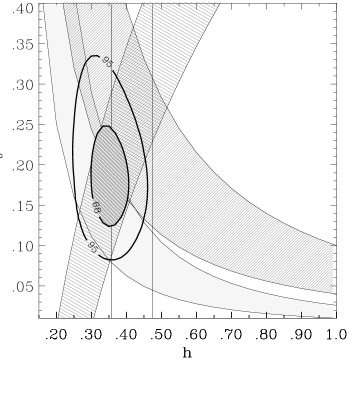
Figure 1.: This plot is from Lineweaver et al. (1997). It gives the region of the h- $\Omega_{b}$ plane allowed by various constrains:BBN, cluster baryonic fraction (White et al.), and the shape parameter ${\Gamma}$ from galaxy and cluster scale density fluctuations. A low h value is preferred

Other possible solutions are:
1.- The calculations of standard primordial nucleosynthesis are incorrect.
2.- The X-ray gas is more concentrated with respect to the dark matter but White et al.(1993) have shown that gravitational and dissipative effects during cluster formation cannot account for such baryon overdensity.
3.- The intracluster gas is multi-phase, but no model has been proposed to explain such a clumpy configuration of the gas.
4.- There is a problem with the mass estimates. This solution will be discussed in next sections.

Finally, one may ask another interesting question. Is the baryon fraction the same in all clusters ? In the standard picture of cluster formation driven solely by gravitational instability and where cluster evolution is entirely self-similar, the expected baryon fraction should be constant, because no segregation between the gas and dark matter has occured. However, if we gather all the derived baryon fractions in the literature and compare them, the answer is clearly NO. For example the derived mean values of WF and DJF samples are different, 15% for the former and 20% for the later (but see Evrard 1997). More recently, Lowenstein & Mushotzky (1996) have shown evidence of variations in baryon fraction from their analysis of two poor Abell clusters, A1060 and AWM 7, using the most recent X-ray observations from ROSAT and ASCA (Figure 2). Such variation in baryon fraction from cluster to cluster requires some process in addition to gravity, like feedback mechanisms or some other non-gravitational effects as suggested by DJF, but there are no theoretical arguments justifying such ideas (White et al. 1993).

Figure 2.: This plot is taken from Lowenstein & Mushotzky (1996). It gives the enclosed baryon fraction versus radius in units of the virial radius in A1060 and AWM7. The dotted (solid) line represents the best-fit mass model, the dot-dashed (dashed) lines the most compact and diffuse models for A1060 (AWM 7). The compact models lie below the best fits.

3. The dark matter problem

Galaxies and hot gas are only a small part of the total cluster mass. The dominant component is the dark matter. Zwicky in 1933 then Smith (1936) have shown that the virial mass exceeds by a large factor the luminous mass. This led them to invoke for the first time, the problem of missing mass. To quantify the amount of dark matter, we usually calculate the mass-to-light ratio (MLR). The mean value found for rich clusters using blue luminosties is $M/L_{B}\approx 300{\sl h}$. In this unit the $M/L{{}_{B}}$ required to close the Universe is $\sim 1200{\sl h}$. Therefore, if we assume that clusters of galaxies are good tracers of the whole Universe, then $\Omega_{0}=0.2-0.3$. So, if one believes in a matter dominated flat cosmological model ${\Omega_{0}}=1$, then where is the missing mass? Still now we do not know how the dark matter is distributed relatively to the visible matter. Cluster mass determinations using optical observations are based on the assumption that mass follows the light distribution which is just an assumption not yet confirmed. What are the predictions on the mass distribution? Cosmological theories predict that dark matter is more diffusely distributed than galaxies. West and Richstone using N-body simulations have indeed confirmed this behaviour (West & Richstone 1988). Furtheremore Hughes (1989), using X-ray observations of the Coma cluster, has shown that models where dark matter parallels the distribution of hot gas are ruled out by the data. With the improvement of weak lensing analysis, one may hope that this question will be answered more precisely, in the near future.

4. Mass determinations

In this section, I will review the methods used to estimate clusters masses and will discuss their validity.

4.1. Optical methods

The Virial Theorem method

:

Early estimates of cluster masses (before X-ray observations became possible) were based on the application of the Virial theorem. If one assumes that clusters of galaxies are bound and self-gravitating systems then the virial mass is given by:

$$M_{v}{\sim 3\frac{R{{}_{G}}{\sigma}{{}_{r}}{{}^{2}}}{G}},$$ (4)

where ${\sigma}^{2}$ and ${R_{G}}$ are evaluated from the radial velocity distribution (2) and the projected spatial distribution of a fair sample of galaxies. As we have seen the naive application of equation(4) leads to large amounts of dark matter. Therefore the question we want to address here is: How secure are the virial mass estimates? Projection effects, contamination by foreground galaxies and anisotropy of the velocity distribution may introduce uncertainties into the determination of the mass. But they are small effects and can not explain such large virial masses. Several observations at both optical and X-rays wavelengths provide convincing evidence of the presence of substructure in a large sample of clusters (Baier 1983, Bird, 1994, Mohr et al. 1993). X-ray imaging observations with the Einstein satellite first revealed such complex structure (Forman et al. 1981) in contrast to the smooth shape assumed in previous studies. Even clusters that exhibit a fairly smooth and apparently well-relaxed configuration , like the Coma cluster, have been found to contain substructure (Fitchett & Webster 1987, Mellier et al. 1988) with a large subcluster centered on NGC 4839 that appears to be falling into the Coma cluster. If this subclustering is not correctly taken into account, this would introduce large uncertainties in the dynamical mass. A substructure with 10% of the mass can introduce an underestimation of 40% on the MLR.
However, the most serious problem of using the virial theorem comes from the fact that we do not know how the dark matter is distributed. Indeed, the application of the standard virial theorem assumes that mass follows the light distribution. What happens when this assumption is relaxed? It has been shown (Sadat 1995) that in this case the standard application of the virial theorem introduces a bias on the cluster masses, and this bias (${\mu}=(M/L)_{\sl dyn}/(M/L)_{\sl true}$) depends strongly and in a non-linear way on the relative concentrations of the visible and invisible components. It is found that the cluster mass is over-(under) estimated if the dark matter is more (less) concentrated by an amount

$${\mu}=\frac{{[1+2C{{}_{c}}R_{\sl true}+C_{\lambda}R_{\sl true}^{2}}]}{[1+C{{}_{v}}R_{\sl true}]},$$ (5)

where $R_{\sl true}$ is the true ratio of the masses $M_{\sl DM}/M_{\sl gal}$ and $C_{v}$, $C_{\lambda}$, $C_{c}$ are the relative concentrations of the 2 components. As an illustration of this effect we have plotted in Figure 3 the bias ${\mu}$ versus $R_{\sl true}$ in the case where the dark matter is less concentrated than the galaxies.

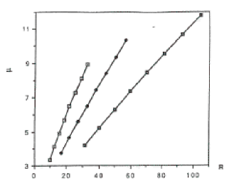
Figure 3.: The bias ${\mu}$ versus the true ratio ${R=R_{true}}$ of ${dark/luminous}$ mass in the case where the mass is more diffusely distibuted than galaxies. The three curves correpond to different concentrations

Figure 4.: Logarithm of the true ratio R versus the bias ${\mu}$ in the case where the mass is more concentrated than galaxies.

Figure 3 shows that for a ratio of, say, $R_{\sl true}{\sim 30}$, the virial theorem leads to a dynamical ratio ${\sim 3}$ to 7 times lower. In this case the virial mass determination underestimates the true mass, while in the case where the dark matter is more concentrated (Figure 4) the dynamical ratio reaches the value of ${\mu}$ ${\sim 100}$ which is 3 times higher than the true value ${\sim 30}$!. The true mass is overestimated. Note, that in the mass- follows- light case, $C_{c}=C_{\lambda}=C_{v}=1$ and ${\mu}$= 1 + $R_{\sl true}$. If one defines a new quantity $R_{dyn}={\mu}-1$ which measures the virial estimated ratio of dark matter mass to visible mass, one can see that in this case $R_{dyn}=R_{\sl true}$ and therefore that the virial mass is equal to the true mass. It seems clear from this analysis, that as long as we do not know anything on the distribution of dark versus visible matter, one has to be “sceptical” about the masses derived from the “virial” method.

Kinematic method

If the system is in equilibrium, one can use the equation of stellar hydrodynamics to derive the mass

$$M(<r)=\frac{-Gn_{\sl{gal}}(r)}{r^{2}}\left[\frac{dn_{\sl{gal}}(r)}{dr}{\sigma}_{r}(r){{}^{2}}+\frac{2n_{\sl{gal}(r)}}{r}[{\sigma}{{}_{r}}(r){{}^{2}}-{\sigma}{{}_{t}}(r){{}^{2}}]\right].$$ (6)

For isotropic orbits, ${\sigma}_{r}$ =${\sigma}_{t}$, there would be a unique solution. Unfortunately the orbits of the galaxies are poorly known. Therefore, we have to solve this equation with three unknown quantities: ${\sigma}{{}_{r}}(r)$, ${\sigma}{{}_{t}}(r)$ and M(r). Generally, it is assumed that either ${\beta}(r)=1-{\sigma}{{}_{t}}(r)^{2}/{\sigma}{{}_{r}}(r)^{2}$ and M(r) are known functions and then derive $n_{\sl gal}$ and ${\sigma}{{}_{r}}(r)$ from eq. (6) which are consistent with observations. Unfortunately, the observed velocity dispersion profiles of clusters of galaxies are poorly known and can not put strong constraints on the mass. Indeed, even for the best studied Coma cluster, Merritt (1994) has shown that the observed velocity dispersion profile of this cluster is consistent with several mass distributions.

4.2. The hydrostatic isothermal ${\beta}$-model

Problems encountered with optical methods like the shapes of galaxy orbits, the small number of galaxies in a cluster, effects of contamination and projection can be avoided by using the observations of the hot X-ray emitting gas. The gas can be treated as an isotropic fluid, since the elastic collision times for ions and electrons are much shorter than the timescales for cooling and heating. The timescale required for a sound wave in the intracluster gas to cross a cluster is given by $t{{}_{X}}=1.3[T_{\sl gas}/10{{}^{8}}]^{-1/2}[R/1Mpc]$ Gyr.
Furtheremore, since this time is shorter than the dynamical time of the cluster (${\sim 10}$ Gyr), the gas can be assumed to be in hydrostatic equilibrium with the cluster potential (Sarazin 1986).
Under the assumption of spherical symmetry the equation of hydrostatic equilibrium (balance between the pressure and the gravitational forces) can be solved for the mass interior to r, M(r):

$$M(r)=-\frac{kT_{gas}}{G{\mu}m{{}_{p}}}\left[\frac{dlog{\rho}_{gas}}{dlogr}+\frac{dlogT_{gas}}{dlogr}\right],$$ (7)

where $T_{gas}$(r) and ${\rho}_{gas}$(r) are the temperature and the gas density profiles, k is Boltzmann’s constant, and ${\mu}$ $m{{}_{p}}$ is the mean molecular weight of the gas. In principle, the knowledge of $T_{gas}$ and ${\rho}_{gas}$ from the observations, directly yields the actual mass distribution M(r). This method has several advantages over the optical approach. The gas is isotropic, there are no contamination effects and the most important advantage is that the mass distribution is derived directly without any assumption about the dark matter distribution as is the case with the optical method.
The sad point is that one must recover three dimensional profiles from projected profiles. For the temperature information, this requires the measurement of $T_{gas}$(r) which is still very difficult to obtain, even with the ASCA satellite. In practice, we assume that the gas is isothermal at a mean temperature ${T_{X}}$. Numerical simulations (Evrard 1996) and recent ASCA results (Ikebe et al. 1994) seem to support this assumption at least out to a radius of 1.5 Mpc. If the gas is isothermal, $\rho_{gas}\propto{n_{gal}^{\beta}}$, then the gas distribution is given by the following (Cavaliere & Fusco-Femiano 1976)

$$\rho_{gas}={\rho}_{gas}(0)[1+(R/R_{c})^{2}]^{-3{\beta}/2},$$ (8)

where $R_{c}$ is the core radius and ${\beta}$ is given by,

$${\beta}=\frac{{\mu}m_{p}{\sigma}{{}^{2}}}{kT_{x}},$$ (9)

and ${\sigma}$ is the line of sight velocity dispersion. Both quantities are derived from the observed surface brightness profile which is found to be well characterized by a simple analytical form:

$$S(x)=S_{o}[1+(x/R_{c})^{2})]^{-3{\beta}_{fit}+1/2}$$ (10)

This functional form gives relatively accurate fits to the data (Jones & Forman 1984) except in the central regions of clusters where cooling flows occur. Typical values of ${\beta}_{fit}{\sim}2/3$ are smaller than the value obtained using (9) from the measurements of ${T_{x}}$ and ${\sigma}$. This discrepancy is the so called ${\it\sl{\beta}-problem}$ and has been thoroughly discussed in the litterature. Some solutions have been suggested to solve this problem (Bahcall & Lubin 1994, Evrard 1990, Navarro et al. 1995) see also Gerbal et al. (1995). Smaller than this typical values are obtained by Durret et al. 1995 with a mean value around 0.4. In their work, Durret et al. have analyzed a sample of 12 Einstein clusters with an improved method (Gerbal et al. 1994) of analysis which derives the density and temperature profiles of the X-ray gas by comparing a real cluster X-ray image to a ”synthetic” image for which the counts predicted to be detected by the IPC was calculated by taking into account all the characteristics of the detector such as the point spread function, the effective area as a function of radius and energy. The ellipticity of the cluster is also taken into account. The resulting simulated images are fitted pixel per pixel to observed ones by minimizing the following function :

$${\it{X^{2}}}={\sum}{\sum}\frac{(N_{\sl IPC}(b)-N_{\sl cts}(b))^{2}}{N_{\sl cts}(b)}$$ (11)

A consequence of such flat (small ${\beta}$) gas density profiles is the derived gas mass to dynamical mass ratios (baryon fraction) which are exceedingly large. Another interesting result of this analysis is the highly centrally peaked dark matter distribution in good agreement with the results based on the imaging and modelling of gravitational arcs in clusters (Tyson et al. 1990, Hammer 1991, Mellier et al. 1993, Wu & Hammer 1993).
Using isothermality and (8), equation (7) becomes :

$$M(r)=3{\beta}/G\frac{kT_{X}r}{{\mu}m_{p}}\frac{(r/r_{c})^{2}}{1+(r/r_{c})^{2}}$$ (12)

with ${{\mu}=0.59}$. This method has been extensively used to derive cluster masses, but still one may ask how secure this method is?
The accuracy of the hydrostatic, isothermal “beta-model” method has been examined through hydrodynamical numerical simulations (Schindler et al. 1995, Evrard 1996). In particular, Evrard has shown that this method gives remarkably accurate masses inside a radius between 0.5-2.5 Mpc but with a large scatter (15 - 30%) (Figure 5).

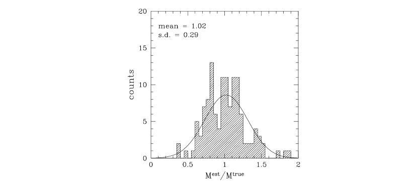
Figure 5.: Histograms of the estimated mass from the ${\beta}$ model from Evrard 1996

However, Bartelmann and Steinmetz (1996) have reached the opposite conclusion, they have found from their gas-dynamical simulations that the ${\sl{\beta}-model}$ yields systematically low cluster mass estimates .
Furtheremore, Balland & Blanchard (1995) have discussed the validity of using equation (7) to infer the mass M(r) from the observed temperature T(r). They argue that the hydrostatic equilibrium equation is unstable and, using a Monte-Carlo procedure, that the resulting accuracy of the mass estimates is rather poor; larger than generally claimed. Applying their procedure to the Coma cluster, they find a factor of at least 2 uncertainty in the mass inside the Abell radius, even when the measurement of the temperature is improved using ROSAT data (Figure 6). An alternative way to go round the ${\beta}-model$ i.e the surface brightness fitting is not required, has been suggested recently by Evrard (1996). This new method exploits an interesting result of his simulations, that is the tight relation between the mass and the temperature and uses the resulting scaling relations: $r_{500}(T_{X})\propto{T_{X}^{1/2}}$ and $M_{500}(T_{X})\propto{T_{X}^{3/2}}$ which lead to more accurate masses and the scatter found in the ${\it\sl{\beta}-model}$ is then eliminated (Figure 7). Of course such conclusions are given in the frame of numerical simulations which simulate clusters in “somehow” perfect conditions. For example their analysis uses the clusters emission- weighted temperature which comes from their simulations and not from cluster spectra. Furthermore, the simulated X-rays images can be analyzed out to large radii which is not generally the case in real observed X-rays ones. Finally, the ${\it\sl{\beta}-model}$ method is based on the assumption of spherical symmetry. However, more often clusters exhibit a more complex morphologies due to the presence of substructures. Numerical simulations have demonstrated that masses of clusters which are undergoing a merging event, are generally under-estimated because part of the energy of the gas is in the kinetic form due to the bulk motion rather than in the thermal form, therefore the temperature of the gas is underestimated and so are the clusters masses. The underestimation of the mass due to the presence of substructure can reach 40% (Schindler 1996).

Figure 6.: This plot shows how the mass profile is poorly constrained by observed temperature profiles even with the recent results on Coma cluster from ROSAT (Briel et al. 1992)

Figure 7.: Histograms of the estimated mass from the scaling law from Evrard 1996

4.3. The Gravitational lensing mass estimates

The discovery of giant blue luminous arcs in clusters A370 and Cl 2244-02 (Soucail et al. 1987, Lynds & Petrosian 1989) has provided the first observational evidence that clusters of galaxies may act as gravitational lenses on background galaxies, a possibility which was first discussed by Noonan (1971). Gravitational lensing provides a very powerful tool to directly measure the projected mass distribution. This method, presents many advantages over the X-ray mass estimates, for example, it does not require any assumption on the mass distribution or on the dynamical state of the cluster. Since the pionnering work by Tyson et al. (1990). It has become more and more common to use weak gravitational lensing to map the dark matter distribution in clusters. Detailed study of image formation through gravitational lensing can be found in the review by Schneider, Ehlers and Falco ( 1992) and Fort & Mellier (1994). I will just summary very briefly the manifestations of the lensing effect and the way the lensing masses are derived. The lensing effects can be divided into two main regimes depending on the lens configuration :

1-The strong lensing regime :

The distorsion of distant galaxies by foreground clusters of galaxies gives rise to the spectacular strong arcs observed in the central regions of clusters e.g. A370 corresponding to a large magnification and strong distorsion. The arclet regime is intermediate between the arc and the weak distorsion regimes.
2-The weak lensing regime or weak shear:

The first observational detection using optical galaxies as sources is due to Tyson, Valdes and Wenk (1990). In this case, each source produces only one image which experiences only a weak distorion of its shape.
The strong lensing regime constrains the total mass enclosed within the “ Einstein radius”, while weak shear effects determine the distribution of the mass at the outer regions (see Brainherd in these proceedings).

Constraints from Strong Lensing

The projected cluster mass within the Einstein radius $r_{E}$ of arc or arclet can be easily derived if one assumes a spherical matter distribution for the lensing cluster and assuming that the system observer-lens-source is aligned along the line of sight

$$M_{\sl lens}={\pi}r_{E}^{2}{\sum}_{\sl crit},$$ (13)

where ${\sum}_{\sl lens}=\frac{c^{2}}{4{\pi}G}\frac{D_{s}}{D_{\sl l}D_{\sl ls}}$ is the critical mass density with ${D_{s}}$, ${D_{\sl l}}$ and ${D_{\sl ls}}$ being the distance to the source (the galaxy), distance between the source and the lensing cluster and the distance between the source and the cluster respectively. For more complex configurations, cluster masses are estimated by lens modelling (see Fort & Mellier 1994 for a review). This method, however gives the mass inside the radius where the arcs are observed which are usually very small ${\approx 50}$ kpc.

Constraints from weak lensing

To construct the surface mass density profile one uses the statistic suggested by (Fahlman et al. 1994)

$${\chi}(r_{1},r_{2})=\overline{\sum}(r_{1})-\overline{\sum}{(r_{1}<r<r_{2})}=\frac{2\sum_{\sl crit}}{1-r^{2}_{1}/r^{2}_{2}}\int_{r_{1}}^{r_{2}}<{\epsilon}>dlnr$$ (14)

where $<{\epsilon}>$ is the mean tangential component of the image ellipticities. This method has been successfully applied to several clusters (see Table 1). How reliable is the lensing method? The main shortcomings of the lensing method is that the application of equation (14) requires an estimation of ${\sum}_{\sl crit}$ and therefore the knowledge of the redshift of the sources which is difficult to obtain. This may introduce large uncertainty in the mass especially for distant clusters. On the other hand it is not possible to obtain a true value of the mass only from the shear map, even in the best case where the sources redshift is known because of the degeneracy due to the fact that the addition of a constant mass plane does not induce any shear on background galaxies. This degeneracy may be broken by measuring the magnification ${\mu}$ of the background which gives an absolute measurement of the mass. Broadhurst et al. (1995) have proposed a very nice method to measure ${\mu}$ by comparing the number count in a lensed and unlensed field. They find that depending on the slope of the number count in the reference field s=dlogN(m)/dm, they observe more or fewer objects in the lensed field. In the case where blue galaxies are selected, the counts are unaltered, since the slope is in this case equal to the critical value s=0.4. This method has been applied successfully to the cluster A1689 by Broadhurst (1995). The weakness of this method is that it requires the measurement of the shape, size and magnitude of very faint objects. Van Waerbeke et al. (1996) have recently suggested a new method to analyz¡e the lensing effects which avoids the measurement of the shape parameter. But still, the weak lensing method leads to very encouraging results and promises to yield unambigeous information about the mass distribution in the near future.

4.4. Comparison between X-ray and lensing cluster mass estimates

Miralda-Escudé & Babul (1995) have raised an interesting puzzle. They found from their analysis of Abell clusters A2218, A1689 that the mass in the central part of the cluster inferred from the strong lensing method is greater than that derived from the X - ray method by a factor of 2 - 2.5. Wu & Fang have gathered all the clusters for which the mass has been estimated and compared the X-ray to lensing masses. They have found a systematic discrepancy between the two masses at small radius ${\approx 0.25}$ ${h_{50}^{-1}}$ Mpc which vanishes at larger radii. However the lensing and the X-ray information in their sample do not come from the same cluster. Early studies based on both optical and lensing observations have led to the same conclusion: there is a cluster mass discrepancy by the same factor (Wu  Fang 1994, Fahlman et al. 1994). But, it seems from a recent statistical analysis that virial masses are consistent with gravitational lensing masses (Wu & Fang 1997). The disagreement between the lensing masses and X-ray masses may be due to the fact that X-ray analysis, namely the ${\sl{\beta}-model}$, underestimates the masses. Indeed, the assumption of hydrostatic equation may be invalid, because of several reasons, non-thermal pressure, merging effects, a multi-phase medium, unstability of the equilibrium equation etc…Unfortunately, it is hard to quantify all these effects and to know which is the most important one.

cluster	$Redshift$	arc/w.l.	$r$(Mpc)	$m_{lens}$	ref.
A370	0.374	arc	0.16/0.4	2.9/12.	1
A1689	0.17	arc/w.l.	0.19/3.	3.6/89.	2,3
A2163	0.201	arc/w.l.	0.066/0.9	0.41/$13_{-7}^{+7}$	4,5
A2218	0.175	arc/w.l.	0.085/0.8	0.61/7.8	6
A2219	0.225	arc	0.1	1.6	7
A2390	0.231	arc/w.l.	0.18/1.15	1.6/$19.5_{-6.5}^{+6.5}$	8,9
CL0500	0.316	arc	0.15	1.9	10
CL0024	0.391 E	arc/w.l	0.22/3.0	3.6/40.	11,12
CL0302	0.423	arc	0.12	1.6	13
CL2244	0.328	arc	0.06	0.25	14
MS1224	0.33	w.l.	0.96	7.0	15
MS1054	0.83	w.l.	1.9	$28_{-6}^{+6}$	16
AC114	0.31	arc	0.35	13	17
PKS0745	0.103	arc	0.046	0.30	18
RXJ1347	0.451	arc	0.24	6.6	19

Table 1.: Lensing masses for a sample of clusters. ${\bf Ref.}$ (1)Kneib et al. 1993; (2,3) Tyson & Fisher 1995; (4,5) Miralda-E & Babul 1995, Squires et al. 1996a; (6) Kneib et al. 1996,(7) Smail et al. 1995b; (8,9) Pello et al. 1991, Squires et al. 1996b;(10) Giraud 1988; (11, 12) Wallington & Kochanek 1995, Bonnet et al. 1994; (13)Mathez et al. 1992,(14) Hammer et al. 1989, (15) Fahlman et al. 1994; (16) Luppino & Kaiser 1996;(17)Smail et al. 1995a; (18) Allen et al. 1996; (19)Schindler et al. 1995

5. Discussion and conclusion

Dynamical analysis of clusters of galaxies have led to two important results: the presence of large amount of dark matter and the evidence of high baryonic fraction, both have implications on cosmology through ${\Omega}_{0}$ and ${\Omega}_{b}$, the density of the Universe and its baryon content respectively. Estimating the masses of clusters of galaxies, is not straightforward, because it depends on the validity of the assumptions underlying the method from which the mass is determined, the mass-follows-light in the case of the virial masses, the hydrostatic equilibrium and isothermality of the gas for the X-ray mass determination. Gravitational lensing methods provide with a new strong tool to constrain both the amount of mass and its distribution. Comparing the X-rays to lensing masses give rise, at least in the inner part of the cluster, to the mass discrepancy problem. The most probable explanation, would be the underestimation of the X-ray mass. The interesting implication, is that clusters would be more massive than we think, and the ratio of gas mass to total mass (the fraction of baryons) could be in more better agreement with nucleosynthesis predictions and an ${\Omega}_{0}$=1 Universe. Finally, thanks to new recent set of observations, it appears that virial masses are in good agreement with the lensing masses (Wu & Fang 1997), if this result is true, that means that the virial masses are accurate and one may conclude that indeed, the mass follows light, since it is only in this case that the virial method gives accurate mass determination (Sadat 1995).

Acknowledgments.

First I would like to thank Drs. K. Chamcham, M. Henry and D. Valls-Gabaud for the invitation to the School. I’m grateful to C. Balland, C. Lineweaver, X.P. Wu, and A. Evrard, for providing the postscript files of their figures (I apologize for the rather poor quality of the few scanned figures). Finaly, I would like to thank our morrocan hosts for their hospitality. This work was supported by the French Ministère National de l’Enseignement Supérieur et de la Recherche.

References

Allen, S. W., Fabian, A. C., & Kneib, J. P., 1996, MNRAS, 279, 615

Arnaud, M., 1994, in Clusters of Galaxies, Proceedings of the XXIXth Rencontres de Moriond, p.211

Bahcall, N.A. & Lubin, L.M., 1994, ApJ 426, 513

Baier, 1983, Astr. Nach., 304, 211

Balland, C. & Blanchard, A., 1997, ApJ in press

Bartlett, J.G., Blanchard, A., Silk, J. & Turner, M.S., 1995, Science, 267, 980

Bartelmann,M. & Steinmetz, M., 1996, MNRAS, 283, 431

Bird, 1994, ApJ, 422, 480

Böhringer, H., 1994, in Cosmological Aspects of X-ray Clusters of Galaxies, W.C. Seitter (ed.), Kluw. Publ.

Bonnet, H., Mellier, Y., & Fort, B. 1994, ApJ, 427, L83

Broadhurst, T., Taylor, A.N., Peacock, 1995, ApJ, 438, 49

Broadhurst, T., 1996, astro-ph/9511150

Briel, U.G., Henry, J.P. & Böhringer, H., 1992, A & A, 259, L31

Cavaliere, A. & Fusco-Femiano,R., 1976, A & A, 49, 137

Durret, F., Gerbal, D., Lima-Neto, G., Lachièze-Rey, M. & Sadat, R., 1994, A & A, 287, 733

David, D., Forman, W. & Jones, C., 1990, ApJ, 356, 32

Evrard, A.E., 1990, ApJ, 363, 349

Evrard, A.E., Metzler, C., Navarro, J.F., 1996, ApJ, 469, 494

Evrard, A.E., 1997, astro-ph/9701148

Fahlman, G.,Kaiser, N., Squires, G., and, Woods, D., 1994, ApJ, 437,56.

Fitchett,M. & Webster,R.,1987, ApJ, 317, 653

Forman, W. et al. 1981, ApJ Lett., 243, L133

Gerbal, D., Durret, F., Lima-Neto, G., Lachièze-Rey, M., 1992, A & A, 253, 733

Gerbal, D., Durret, F., Lachièze-Rey, M., 1994, A & A, 288, 746

Giraud, E., 1988, ApJ, 334, L69

Hammer, F., 1991, ApJ, 383, 66

Hughes, H., 1989, ApJ, 337, 21

Ikebe,Y. 1994, in Clusters of Galaxies, Proceedings of the XXIXth Rencontres de Moriond, p.163

Jones,C. & Forman,W., 1982, ApJ, 276, 38

Lineweaver, C., Barbosa, D., Blanchard, A. & Bartlett, J., 1997, astro-ph9612146

Lowenstein, M. & Mushotzky,R.F., 1996, astro-ph/9608111

Lynds, R. & Petrosian,V., 1989, ApJ, 336, 1

Mellier, Y. et al., 1993, ApJ, 407, 33

Mellier, Y. & Fort, B., 1994, A & A Rev., 5, 239

Merritt, D., in Clusters of Galaxies, Proceedings of the XXIXth Rencontres de Moriond, p.11

Miralda - Escudé, J., 1991, ApJ 370, 1

Miralda-Escudé, J., & Babul,A., 1995, ApJ, 449, 18.

Mohr, J.J., et al., 1993, ApJ, 419, L9.

Mushotzky, R.F., 1996, in The Rôle of Baryons in Cosmology, Berkeley

Navarro, J.F., Frenk, C., White, S.D.M., 1995, MNRAS, 275, 720.

Noonan, T.W., 1971, Astron.J, 76, 765

Pelló, R., et al. 1991, ApJ, 366, 405

Pierre, M., Soucail, G., Böhringer, H., & Sauvageot, J. L. 1994, A & A289, L37

Rugers, M. & Hogan, C.J., 1996, ApJ, 459, L1

Sadat, R., 1995, Astrophy. & Sp. Science, 234, 303

Sarazin,C.L., 1986, Ann. Rev. Mod. Phys., 58, 1.

Schneider,P. Ehlers, J. & Falco,E.E, 1992, in Gravitational Lenses,

Springer Verlag

Schindler, S. 1996, A & A, 305, 858

Schindler, S. et al. 1995, A & A, 299, L9

Smail, I., Couch, W. J., Ellis, R. S., & Sharples, R. M. ApJ, 1995a, 440, 501

Smail, I., et al. 1995b, MNRAS, 277, 1

Smith, H., 1936, ApJ,83, 23

Soucail, G., Fort, B., Mellier, Y., Picat, J.P.,1987, A & A, 184, L14

Squires, G., et al. 1996a, ApJ, submitted; astro-ph/9603050

Squires, G., Kaiser, N., Fahlman, G., Babul, A., & Woods, D. 1996b, ApJ, 469, 73

Tyson, J.A., Valdes, F., & Wenk, R., 1990, ApJ,349, L1

Tyson, J. A., & Fischer, P. 1995, ApJ, 446, L55

Tytler, D., Fan, X-M. & Burles, S. 1996, Nature, 381, 207

Van Waerbeke, L. & Mellier, Y., 1996, astro-ph/9606100

Walker, T.P, Steigman, G., Schramm, D.N., Olive, K.A., & Ho-Shik Kang, 1991, ApJ, 376, 51

Wallington, S., & Kochanek, C. S. 1995, ApJ, 441, 58

West, D.J. & Richstone, D.O., 1988, ApJ, 335, 532

White, S.D.M.,Navarro, J.F., Evrard, A.E., & Frenk, C.S. 1993, Nature, 366, 429

White, D.A., & Fabian,A.C., 1995, MNRAS, 273, 72

Wu, X.P. and Hammer, F., 1993, MNRAS, 262, 187

Wu, X.P. and Fang, Li-Zhi, 1997, astro-ph/9701196

Wu, X.P. and Fang, Li-Zhi, 1996, ApJ, 467, L45

Zwicky,F. 1933, Helv. Phys. acta,6,110