Gold in the Doppler Hills:
Cosmological Parameters in the Microwave Background
Abstract
Research on the cosmic microwave background (CMB) is
progressing rapidly. New experimental groups are popping up
and two new satellites will be launched.
The current enthusiasm to measure fluctuations in the CMB power
spectrum at angular scales between and
is largely motivated by the expectation that CMB determinations
of cosmological parameters will be of unprecedented precision: cosmological
gold.
In this article I will try to answer the following questions:
What is the CMB?
What are cosmological parameters?
What is the CMB power spectrum?
What are all those bumps in the power spectrum?
What are the current CMB constraints on cosmological parameters?
Observatoire Astronomique de Strasbourg
11 Rue de l’Université
67000 Strasbourg, France
charley@astro.u-strasbg.fr
1. What is the Cosmic Microwave Background?
Thirty years ago Penzias and Wilson (1965) discovered excess noise in their horn antenna in Holmdel, New Jersey. The measured temperature of this noise was K and it did not vary in intensity over the sky; it was isotropic. They received the Nobel Prize for this serendipitous discovery of the cosmic microwave background (CMB) radiation. The prediction of the existence of a CMB and of its temperature (Alpher & Herman 1948) followed by its detection, provides possibly the strongest evidence for the Big Bang.
The observable Universe is expanding and cooling. Therefore in the past it was hotter and smaller. The CMB is the after-glow of thermal radiation left over from this hot early epoch. It is the redshifted relic of the Big Bang. The CMB is a bath of photons coming from every direction with wavelengths about as big as these letters. There are about of them in every cubic centimeter of the Universe. These are the oldest photons one can observe (see Figure 1). Their long journey towards us has lasted 99.997% of the age of the Universe; a journey which began when the photons were last scattered by free electrons of the ubiquitous cosmic plasma, when the Universe was times smaller and the temperature times higher than the CMB is today. The CMB contains
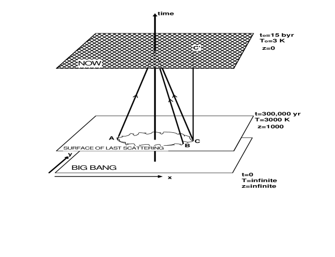
information about the Universe at redshifts much larger than the redshifts of galaxies or quasars. It is a unique tool for probing the early Universe.
To a very good approximation the CMB is a flat featureless blackbody; there are no anisotropies; the temperature is a constant in every direction (KCL) Fixsen et al. 1996). This near isotropy was the reason it took more than 25 years to detect anisotropies in the CMB. However the galaxies around us are clustered on scales from 1 Mpc (our Local Group) up to Mpc (great walls, sheets and voids). If these structures formed from overdensities which gravitationally collapsed, the overdensities must have been present in the early universe and must have produced temperature anisotropies in the CMB. In the Spring of 1992, the COBE DMR team announced the discovery of anisotropies in the CMB (Smoot et al. 1992). Since then the field of CMB-cosmology has blossomed.
2. What are Cosmological Parameters?
2.1. Friedman Robertson Walker (FRW) Universe
Cosmological parameters are the important ingredients of any cosmological model. If we work within General Relativity and add the hypothesis that the Universe is homogeneous and isotropic then the Einstein equations reduce to the Friedmann equation with its relatively few parameters:
| (1) |
-
•
: the scale factor used to parametrize the global expansion (or shrinking) of the Universe. In the Big Crunch (or looking backwards towards the Big Bang) .
-
•
: the present value of Hubble’s parameter. In terms of the scale factor . The units are and it is sometimes written dimensionlessly as . The subscript “o” refers to the present time.
-
•
: the current dimensionless density of component of the Universe expressed in units of the critical density (). Thus for example the physical density of baryons is and the measurement of gives limits on . The critical density marks the boundary between eternally expanding universes and recollapsing universes.
-
•
: the density of relativistic matter, e.g., hot dark matter (HDM), neutrinos and radiation for which . .
-
•
: the density of non-relativistic matter, e.g., cold dark matter (CDM) or baryons, .
-
•
: the total matter density of the Universe, .
-
•
: the curvature density of the Universe. . The factor for the cases of closed, flat or open geometries respectively, corresponding to respectively.
-
•
: vacuum density of the Universe. . The cosmological constant .
Evaluating the Friedmann equation at the present () provides the constraint . Inflation implies that the Universe is flat which means and . In the standard CDM model (flat universe, no cosmological constant, ), equation (1) can be integrated to yield the age of the Universe Gyr. For more generic cases, (see e.g., Kolb & Turner 1990).
2.2. Perturbed FRW
An FRW universe is perfectly isotropic and homogeneous; a boring universe without galaxies, stars or dense perturbations like ourselves. So we need to add perturbations to the model. We parametrize these perturbations in terms of the normalization and slope of the CMB power spectrum. There are two families of perturbations which influence the CMB power spectrum: scalar (= density) perturbations and tensor (= gravitational wave) perturbations, and correspondingly there are 2 normalizations and slopes.
-
•
: the quadrupole normalization of the power spectrum, usually expressed in K. was determined accurately by the COBE satellite. If there are no perturbations. Inflation does not predict this normalization. The tensor analog is .
-
•
: the slope of the primordial power spectrum, observable today at the largest angles. The tensor analog is .
2.3. Summary
The perfectly homogeneous and isotropic FRW model is parametrized by
| (2) |
The total mass density has several components which are also parameters:
| (3) | |||||
| (4) |
Perturbations to the FRW universe are parametrized by
| (5) |
Cosmological parameters are important because they tell us
-
•
the ultimate destiny of the Universe:
-
•
the age and size of the Universe:
-
•
the composition of the Universe:
-
•
the origin of structure
What makes these parameters even more important and what makes CMB-cosmology such a hot subject is that in the near future measurements of the CMB angular power spectrum will determine these parameters with the unprecedented precision of a few % (Jungman et al. 1996).
3. What is the CMB power spectrum?
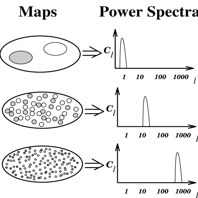
Similar to the way sines and cosines are used in Fourier decompositions of arbitrary functions on flat space, spherical harmonics can be used to make decompositions of arbitrary functions on the sphere. Thus the CMB temperature maps are conveniently written as:
| (6) |
The power spectrum is the sum of the squares of the coefficients
| (7) |
See Figure 2 for a brief initiation. If the matter power spectrum is written in scaleless form as , then the radiation power spectrum at scales larger than a few degrees () becomes (Bond & Efstathiou 1987)
| (8) |
where is the slope of the power spectrum, is the normalizing quadrupole amplitude (analogous to and is just another way of writing ) and sets the angular scale (analogous to the linear scale ). If (as implied by inflation, consistent with the COBE measurements and first proposed by Harrison (1970) and Zel’dovich (1972)), then
| (9) |
thus
| (10) |
This is why the y-axis of CMB angular power spectra are labeled with some function of and why the plotted spectra are flat for (see Figure 3).
3.1. Horizons and Angular Scales
To get a rough understanding of the power spectra in Figure 3, we can divide up the plot into super-horizon and sub-horizon regions as is done in Figure 4. The angular scale corresponding to the particle horizon size is the boundary between super- and sub-horizon scales. The size of a causally connected region on the surface of last scattering is important because it determines the size over which astrophysical processes can occur. Normal physical processes can act coherently only over sizes smaller than the particle horizon and could not have produced the structure in the COBE maps and a fortiori could not have produced the better than one part in homogeneity of the entire CMB sky.
A causally connected Hubble patch at last scattering subtends an angular size (for an observer today) of
| (11) |

.

.
Thus as , and as , (see Figure 5). The angle subtended by an object of size at an angular distance is . Thus the angular scale associated with the peak of the power spectrum is
| (12) |
where is the angular scale of the Doppler peak. The physical scale of the peak oscillations is some fixed fraction of the horizon . The time of decoupling scales as and the angular distance . In flat models and where
| (13) |
Inserting this into equation (12) yields the monotonic relation: when , (see Figure 5b). Equation (12) says that when . The scaling can be understood as the effect of larger universes: a given physical size at a larger distance subtends a smaller angle (see Figures 5 and 5b).
There is structure in the DMR maps on super-horizon scales. How did it get there? Inflation is invoked to explain this apparently acausal structure (see the contribution by Liddle in this volume). If defect models of structure formation are correct then this acausality is only apparent; low defects produced the large scale anisotropies. If inflation is correct, the apparent causal disconnection of the spots in the DMR maps means we are looking much further back than the epoch of last scattering. The structure that one sees in the DMR maps may represent a glimpse of quantum fluctuations at the inflationary epoch seconds after the Big Bang, showing us scales times smaller than the atomic structure seen with the best ground-based microscopes. For more on the DMR instrument as a microscope see Lineweaver (1995).
4. What are all those Bumps in the Power Spectrum
4.1. Decoupling and the Surface of Last Scattering
At about 300,000 years after the bang, the Universe had cooled down enough to allow the free electrons and protons to combine to form neutral hydrogen. This period is known as decoupling. This neutralization of the plasma allowed photons to free stream in all directions. Before decoupling the Universe was an opaque fog of free electrons, afterwards it was transparent. The boundary is called decoupling, recombination, the cosmic photosphere or the surface of last scattering; the surface where the CMB photons were Thomson scattered for the last time before arriving in our detectors.
Decoupling occurs when the CMB temperature has dropped to the point when there are no longer enough high energy photons in the CMB to keep hydrogen ionized; . Although the ionization potential of hydrogen is 13.6 eV ( K) decoupling occurs at K. The high photon to proton ratio () allows the high energy tail of the Planck distribution to

.
Figure 5b. Power Spectra Parameter Dependence The dotted line is the polynomial fit to the data in Figure 3 and is the same in all panels as a reference. Top left: in each panel is fixed while takes on the values indicated. The largest values of have the largest Doppler peaks. Notice that as increases, the peak amplitude increases for large but decreases for small ; thus at high the peak amplitude is an excellent baryometer. Upper right: in each panel takes on the values indicated. Notice that the slope at low and the peak amplitude do not have a simple monotonic dependence on . Lower left: in each panel takes on the values indicated. The largest values of have the largest Doppler peaks. As increases, the peak amplitude decreases and the peak position shifts to larger scales. All models are Harrison Zel’dovich () normalized to the COBE 4-year results. Figures from Lineweaver et al. 1997a, 1997b.
keep the comparatively small number of hydrogen atoms ionized until this much lower temperature (for details check out the Saha equation).
The temperature of the CMB as a function of redshift is . Decoupling occurs at a fixed temperature . As the Universe cools down , thus the surface of last scattering recedes from us with an ever-increasing redshift, .
4.2. Anisotropy Mechanisms in a Perturbed Robertson-Walker Universe
The temperature of CMB photons can be influenced by any field which couples to photons. There are three:
-
•
Gravity , by gravitational red and blue shifts
-
•
Density , by compression heating and rarefaction cooling
-
•
Velocity , by scattering from moving charged particles (Doppler effect).
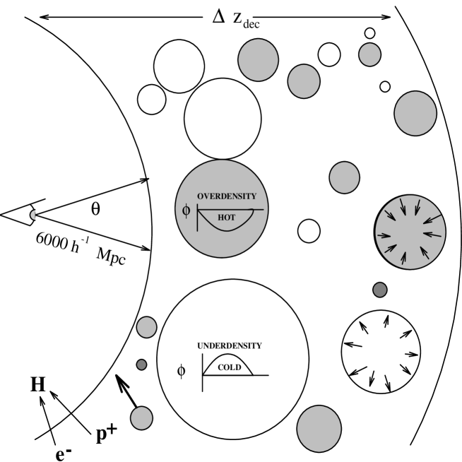
The dominant effects on the CMB produced by these fields occur at the surface of last scattering, i.e., at a distance Mpc from the observer in the direction of the line of sight (Figure 6). The differential temperature of the CMB in direction , , can be expressed as a function of the potential , the density fluctuations and the velocity .
| (14) |
or in words,
| (15) |
Notice that all four terms in equation (14) are independent of the frequency of the radiation. This spectral flatness is used by observers to distinguish CMB anisotropies from Galactic and extragalactic foregrounds. In the next two pages I will try to explain how these different terms influence the CMB on different scales.
4.3. Large Super-horizon Scales
Gravity
On angular scales larger than a few degrees, the cold and hot spots in the CMB maps are caused by the red- and blue-shifting of photons leaving primordial gravitational potential fluctuations (Sachs & Wolfe 1967). That is, photons at the surface of last scattering loose energy climbing out of potential valleys and gain energy falling down potential hills; and these valleys and hills have different amplitudes as a function of position on the sky. Hills produce hot spots while valleys produce cold spots. The Pound-Rebka experiment used the Mossbauer effect and confirmed the existence of a gravitational redshift of magnitude , the first term of equation (14).
.
Density
The initial conditions are usually selected to be adiabatic and less commonly isocurvature. With adiabatic initial conditions the locations of the overdensities in the baryon-photon fluid coincide with the locations of the potential wells. This leads to a partial cancelling of the gravity and density terms (see Figure 6). On super-horizon scales , thus the sum of the gravity and density terms is (gravity wins).
With isocurvature initial conditions the curvature from CDM potential wells is compensated by coinciding underdensities of the baryon-photon fluid. No curvature (= “isocurvature”) is the result. The gravity and density terms do not cancel, in fact they add coherently leading to relatively more power on super-horizon scales compared to the adiabatic case.
Velocity
The term is the standard Doppler effect applied to radiation. The velocity can be conveniently decomposed
| (16) |
where is the velocity of the observer, i.e., the velocity of the Sun with respect to the CMB and is the velocity of the last scattering plasma with respect to the CMB. The Doppler term from produces the large observed dipole, known also as the “Great Cosine in the Sky”. The measurement of this dipole tells us how fast we are moving with respect to the rest frame of the CMB (Lineweaver et al. 1995, Lineweaver et al. 1996). When we make a CMB map and remove the mean, the next largest feature visible at 1000 times smaller amplitude is the dipole. But the amplitude of this kinetic dipole is larger than the anisotropies of the CMB power spectrum.
On large scales equation (14) becomes
| (17) |
When we remove the dipole from the maps we are left with only the combined gravity/density term of the Sachs-Wolfe effect, .
On super-horizon scales, the physical decomposition we are making here is ambiguous, i.e., gauge dependent. One gauge’s adiabatic compression is another gauge’s gravitational redshift, but the observed is gauge independent (see e.g. Hu 1995).
4.4. Small Sub-horizon Scales
Gravity
The integrated Sachs-Wolfe effect is gravitational redshifting when the CMB photons fall into shallow potential valleys and climb out of deep valleys (Figure 7).
The early ISW effect is due to the self-gravity of the photons just after . Since photon potentials do not grow with the same scaling as the non-relativistic matter, . Near decoupling, is non-negligible and if we let , , which means that is larger at decoupling and that the contribution from the Early ISW effect increases.

.
The late ISW effect is also from and is produced in non-flat universes () or when . It is “late” in the sense that in the limit as (late times) the last two terms in the Friedmann equation control the expansion (see Tegmark 1995 and Hu 1995 for more details).
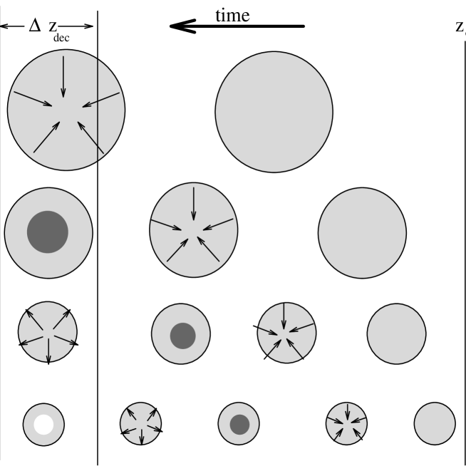
After matter-radiation equality, the growth of CMB potential wells and hills drives acoustic oscillations (see Figure 8).
Density
The correlated combination of density and velocity fluctuations are acoustic waves. Since we are dealing essentially with a single baryon-photon fluid, (the electrons couple the baryons tightly to the photons) adiabatic compression and rarefaction of this fluid creates hot and cold spots that can be seen (Figure 8).
Velocity
Plasma at the surface of last scattering can have a velocity due to bulk motions or to acoustic oscillations which are 90 degrees out of phase with density fluctuations. Figure 8 displays these acoustic oscillations at different scales.
For simplicity, in equation (14), we have assumed a Robertson-Walker metric and therefore do not consider differential expansion as a source of anisotropy. Additionally, we do not include the Vishniac (1987) and Sunyaev-Zel’dovich (1972) effects. These post-decoupling effects contribute to small angular scale anisotropies. We also do not include the more speculative anisotropies due to topological defects (monopoles, strings, walls, textures) or any contribution from a possible rotation of the Universe (Barrow, Juszkiewicz & Sonoda 1985). We also do not include polarization anisotropies. For excellent reviews of this subject and more details see Tegmark (1994), Hu (1995), Bunn (1997) and Hu, Sugiyama & Silk (1997).
5. What are the current CMB constraints on cosmological parameters?
The current enthusiam to measure fluctuations in the CMB power spectrum at angular scales between and is largely motivated by the expectation that CMB determinations of cosmological parameters will be of unprecedented precision. In such circumstances it is important to estimate and keep track of what we can already say about the cosmological parameters. In two recent papers (Lineweaver et al. 1997a & 1997b) we have compiled the most recent CMB measurements, used a fast Boltzmann code to calculate model power spectra (Seljak & Zaldarriaga 1996) and, with a analysis, we have compared the data to the power spectra from several large regions of parameter space.
In Lineweaver et al. (1997a) we considered COBE-normalized flat universes with power spectra. We used predominantly goodness-of-fit statistics to locate the regions of the and planes preferred by the data. In Lineweaver et al. (1997b) we obtained values over the 4-dimensional parameter space for , models. Projecting and slicing this 4-D matrix gives us the error bars around the minimum values. Here we summarize several of our most important results.
One of the difficulties in this analysis is the 14% absolute calibration uncertainty of the 5 important Saskatoon points which span the dominant adiabatic peak in the spectrum (Figure 3). We treat this uncertainty by doing the analysis
.
three times: all 5 points at their nominal values (‘Sk0’), with a 14% increase (‘Sk+14’) and a 14% decrease (‘Sk-14’). Sk+14 and Sk-14 are indicated by the small squares in Figure 3 above and below the nominal Saskatoon points. Leitch et al. (1997) report a preliminary relative calibration of Jupiter and CAS A implying that the Saskatoon calibration should be . Reasonable fits are obtained for Sk0 and Sk-14.
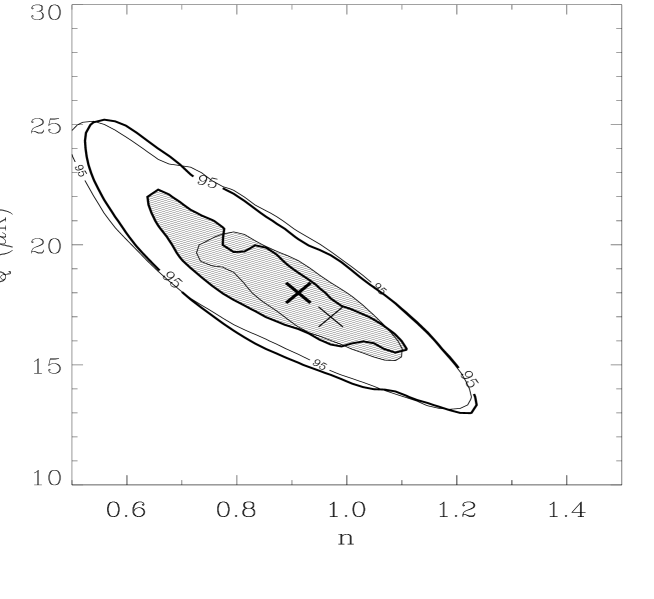
In the context of the flat models tested, our analysis yields: (Figure 9), and K (Figure 10). The and values are consistent with previous estimates while the result is surprisingly low.
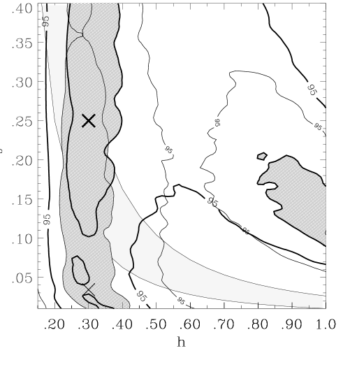
For each result, the other 3 parameters have been marginalized. This result has a negligible dependence on the Saskatoon calibration, i.e., lowering the Saskatoon calibration from 0 to -14% does not raise the best-fitting in flat models. The inconsistency between this low result and results will not easily disappear with a lower Saskatoon calibration. Our results are valid for the specific models we considered: , CDM dominated, , Gaussian adiabatic initial conditions, no tensor modes, no early reionization, K, , no defects, no HDM.
There are many other cosmological measurements which are consistent with such a low value for (Bartlett et al. 1995, Liddle et al. 1996). For example, we calculated a joint likelihood based on the observations of galaxy cluster baryonic fraction, Big Bang nucleosynthesis and the large scale density fluctuation shape parameter, . We obtained .
With two new CMB satellites to be launched in the near future (MAP , Planck Surveyor ) and half a dozen new CMB experiments coming on-line (23 groups), the future looks bright for CMBers ( see Page 1997).
Acknowledgments.
I am grateful to my collaborators D. Barbosa, A. Blanchard and J.G. Bartlett. I want to thank Martin Hendry for his scottish weltanschauuang, David Valls-Gabaud for his anxious professionalism, Khalil Chamcham for his international optimism and Hannah Quaintrell for being there. I am also grateful to Nour-Eddine Najid and Idriss Mansouri of the Faculty of Sciences, Ain-Chock, Hassan II University, Casablanca for helpfully arranging my two public lectures. Wayne Hu made several helpful suggestions. I acknowledge support from NSF/NATO post-doctoral fellowship 9552722.
Discussion
Dr. Liddle: What did you say about ?
Dr. Lineweaver: We can talk about that later.
Dr. Hermit: If what you say is true then everybody else is just plain wrong about the value of Hubble’s constant.
Dr. Lineweaver: Hmmm. We’ll see.
References
Alpher, R. A. & Herman R. C. 1948, Evolution of the Universe, Nature, 162, 774
Barrow, J.D., Juszkiewicz, R. Sonoda, D.H. 1985, M.N.R.A.S., 213, 917
Bartlett, J.G., Blanchard, A., Silk, J. & Turner M.S. 1995, The Case for a Hubble Constant of 30 km s-1 Mpc-1, Science, 267, 980
Bond, J.R. & Efstathiou G. 1987, The Statistics of Cosmic Background Radiation Fluctuations, M.N.R.A.S., 226, 655
Bunn, E. M. 1997, Calculation of Cosmic Background Radiation Anisotropies and Implications, Strasbourg School Proceedings, Kluwer, astro-ph/9607088
Fixsen, D.J. et al. 1996, The Cosmic Microwave Background Spectrum from the Full COBE FIRAS Data Set, Ap. J., 473, 576
Harrison, E.R. 1970, Fluctuations at the Threshold of Classical Cosmology, Phys. Rev. D1, 2726
Hu, W. 1995, Wandering in the Background: A Cosmic Microwave Background Explorer, Ph.D. thesis, U. C. Berkeley
Hu, W., Sugiyama, N. & Silk J., The Physics of Microwave Background Anisotropies, 1997, Nature, in press, astro-ph/9604166
Jungman G. et al. , 1996, Cosmological-Parameter Determination with Microwave Background Maps, Phys. Rev. Lett. 76, 1007
Kolb E.W. & Turner, M.S. “The Early Universe”, 1990, Addison-Wesley
Leitch E. et al. 1997, in preparation
Liddle A. et al. 1996, Pursuing Parameters for Critical-Density Dark Matter Models, M.N.R.A.S., 281, 531
Lineweaver, C. H., Smoot, G. F., Kogut, A., Tenorio, L. 1994, The Cosmic Microwave Background Dipole Anisotropy: Testing the Standard Model, Astrophysical Letters and Communications, 32, 173
Lineweaver, C. H., 1994, Correlation Function Analysis of the COBE Differential Microwave Radiometer Sky Maps, Ph.D. thesis, U. C. Berkeley
Lineweaver, C. H., 1995, Recent COBE Results, in Proc. XXXth Rencontre de Moriond, “Dark Matter in Cosmology, Clocks and Tests of Fundamental Laws”, edt. B. Guiderdoni et al. , 1995, Editions Frontières.
Lineweaver, C. H., Tenorio, L., Smoot, G. F., Keegstra, P., Banday, A. J. & Lubin, P. 1996, The Dipole Observed in the COBE DMR 4 Year Data, Ap. J., 470, 38
Lineweaver, C. H., Barbosa, D., Blanchard, A. & Bartlett J. G. 1997a, Constraints on , and from Cosmic Microwave Background Observations, A&A, (in press), astro-ph/9610133
Lineweaver, C. H., Barbosa, D., Blanchard, A. & Bartlett J. G. 1997b, Cosmic Microwave Background Observations: Implications for Hubble’s Constant and the Spectral Parameters and , A&A, (submitted), astro-ph/9612146
Page, L., 1997, On Observing the Cosmic Microwave Background, astro-ph/97xxx
Penzias A.A. & Wilson, R.W. 1965, A Measurement of Excess Antenna Temperature at 4080 Mc/s, Ap. J., 142,419
Sachs, R. K. & Wolfe, A. M. 1967, Perturbations of Cosmological Model and Angular Variations of the Microwave Background, Ap. J.147, 73
Seljak, U. & Zaldariaga M. 1996, A Line-of-sight Integration Approach to Cosmic Microwave Background Anisotropies, Ap. J., 469, 437
Smoot, G.F. et al. 1992, Structure in the COBE Differential Microwave Radiometer First-Year Maps, Ap. J., 396, L1
Sunyaev, R.A. & Zel’dovich, Y. B. 1969, The Observation of Relic Radiation as a Test of the Nature of X-Ray Radiation from the Clusters of Galaxies, Comments Astrophys. Space Phys. 4,173
Tegmark, M., 1996, Doppler peaks and all that: CMB anisotropies and what they can tell us, Varenna School Proceedings, 1996,astro-ph/9511148
Vishniac, E.T. 1987, Ap. J., 322, 597
Zel’dovich, Y.B. 1972, A Hypothesis Unifying the Structure and the Entropy of the Universe, M.N.R.A.S., 160, 1