Abstract

We study the accretion of cold and hot dark matter onto a cosmic string wake using a high-resolution numerical simulation. We verify previous analytical calculations predicting the radius of bound matter around wakes and inflow velocities of the dark matter, as well as assumptions about the self-similarity of the solution. In cold wakes, we show that self-similarity is approached quickly after a ‘binding’ transition. Hot wakes approach self-similarity rapidly once the free streaming ‘pressure’ falls below a critical value and accretion begins. We also analytically calculate the size of the overdensity in wakes with cold dark matter and compare the results to simulations. We remark that the results derived may be used in testing gravitational numerical codes in the non-linear regime.

1 Introduction

Large-scale structure formation in the cosmic string model is not yet well understood, particularly in the non-linear regime. Until recently, only linear analytical treatments have been available for approximating wake characteristics. Rees ${}^{\cite[cite]{[\@@bibref{}{analbaryo}{}{}]}}$ has analytically calculated some of the non-linear effects of baryons in wakes, particularly at the time of formation.

There have also been some recent numerical attempts at understanding the matter distribution better. Shellard and Avelino ${}^{\cite[cite]{[\@@bibref{}{linwake}{}{}]}}$ have developed Zel’dovich techniques including the source terms from cosmic strings, but this work is only valid on large scales where the perturbations are still linear. Sornborger, et. al. ${}^{\cite[cite]{[\@@bibref{}{baryowake}{}{}]}}$ have simulated non-linear evolution of baryons and dark matter in cosmic string wakes, but their simulations had small grids, and therefore could not resolve non-linear features in the matter distribution well. Their simulations also have the drawback that boundary conditions come into play typically by a redshift of $8$, and therefore assumptions have to be made about the scaling of the matter distribution (i.e. that it is self-similar).

Therefore, what is needed is a confirmation of both linear and non-linear results and evolution of the wakes until the present in order to verify that the assumptions about the growth of the matter distribution in the wake are correct. We would like more accurate analytical expressions for the size of wake overdensities to compare with observations. Also, since cosmic strings with cold dark matter generate too much small scale structure ${}^{\cite[cite]{[\@@bibref{}{coldspect}{}{}]}}$, an investigation of the effects of the accretion of hot dark matter would be desirable.

In this paper, we have done high-resolution one-dimensional numerical simulations yielding precise comparisons with the Zel’dovich approximation in the linear regime. In addition, we have extended the Zel’dovich approximation, in a slightly modified guise, to make predictions for the width of the overdensity in the wake into the non-linear regime. We have also extended our simulation to include the effects of hot dark matter.

The cosmic string model of large-scale structure is motivated by the fact that supermassive strings are a common product of a GUT scale phase transition. A string network is formed at the phase transition. The energy carried by the defects curves spacetime, and thus seeds structure formation. Simple arguments ${}^{\cite[cite]{[\@@bibref{}{stringscale}{}{}]}}$, verified by numerical simulations, show that the string network rapidly evolves to a scaling solution. That is, the number of long strings per horizon volume is statistically constant (i.e. when we average over many volumes).

Numerical simulations have shown that cosmic string loops have a typical radius at the limit of resolution of cosmic string network simulations $R\sim 10^{-2}H^{-1}$, whereas there are $\sim 10-30$ horizon sized long strings per particle horizon volume in the matter era ${}^{\cite[cite]{[\@@bibref{}{stringsim1}{}{}]},\cite[cite]{[\@@bibref{}{stringsim2}{}{}]},\cite[cite]{[\@@bibref{}{stringsim3}{}{}]}}$. This indicates that the primary structure formation mechanism in the cosmic string model is in the form of sheetlike wakes formed in the path of long strings.

The matter perturbation caused by a moving long cosmic string comes from two conceptually distinct components of the gravitational field ${}^{\cite[cite]{[\@@bibref{}{stringgrav1}{}{}]},\cite[cite]{[\@@bibref{}{stringgrav2}{}{}]},\cite[cite]{[\@@bibref{}{stringgrav3}{}{}]}}$: a velocity kick imparted to particles toward the plane traversed by the cosmic string due to converging geodesics in the conical spacetime around the string, and a Newtonian field due to the effective mass of small-scale structures such as waves and kinks moving on the string. In linear theory, the comoving velocity impulse toward the wake imparted to a particle after a string has passed by is

$$v_{kick}=-\frac{2\pi G(\mu_{eff}-T)}{v_{s}\gamma_{s}}-4\pi G\mu_{eff}v_{s}\gamma_{s}$$

where $G$ is Newton’s constant, $\mu_{eff}$ is the effective mass-per-length of the string, $v_{s}$ is the velocity of the string, $\gamma_{s}$ is the relativistic gamma factor $\gamma_{s}=(1-v_{s}^{2})^{-1/2}$ and $T$ is the tension on the string which obeys an effective equation of state $\mu_{eff}T=\mu_{0}$. For strings formed at a GUT phase transition, $G\mu_{0}\sim 10^{-6}$. In the expression for $v_{kick}$, the first term comes from the Newtonian field and the second from the deficit angle of the spacetime. Thus, we can see that for fast moving strings ($v_{s}\sim 1$) the impulse from the Newtonian field is negligible compared to that from the deficit angle in the conical spacetime around the string.

To study matter accretion in cosmic string wakes, planar symmetry is often assumed as a first order approximation for ease of calculation. That is, we assume the wake to be formed by a cosmic string in the regime where the string velocity is relativistic (a good approximation) and the string straight (a good approximation if we neglect small scale structure on the strings, which is at present not well understood ${}^{\cite[cite]{[\@@bibref{}{stringsim1}{}{}]},\cite[cite]{[\@@bibref{}{stringsim2}{}{}]},\cite[cite]{[\@@bibref{}{stringsim3}{}{}]}}$, but can be hoped to be of the order of the cosmic string loop scale $<10^{-2}H$). Thus, we neglect the Newtonian field of the string, and we assume that the string has passed through the volume of interest without deviating from being straight, such that the inflow is effectively one-dimensional. In this scenario, two matter streams are formed about the axis where the cosmic string has passed, each with identical velocities toward the axis.

Analytical calculations using the Zel’dovich approximation ${}^{\cite[cite]{[\@@bibref{}{zel}{}{}]},\cite[cite]{[\@@bibref{}{cosstrwake}{}{}]}}$ and assuming planar symmetry have shown that the wake width should grow as $t^{2/3}$ in the matter dominated era. In these calculations, the comoving wake width was defined as the physical radius $h$ from the wake at which the particle turns around ($\dot{h}=0$). For hot dark matter, the width of the wake has been calculated including the effects of the larger phase space volume occupied by dark matter. These calculations predict that hot dark matter wakes laid down at a $t_{eq}$ will be of a size the same order as that of cold dark matter wakes laid down at the same time.

Since the perturbation overdensity $\delta\rho/\rho=1$ in the wake immediately following passage of the string, the solution is non-linear ab initio inside the overdensity. For times $t\gg t_{i}$, where $t_{i}$ is the formation time of the wake, it can be shown that matter accretion has no preferred length or time scales, thus the matter distribution in the wake approaches self-similarity.

In this paper, we study planar symmetric wakes numerically and derive and compare where we can with analytical results. We have developed a high-resolution one-dimensional particle-mesh code to study hot and cold dark matter accretion in cosmic string wakes in the non-linear regime. The calculations are done assuming a matter dominated background.

In the next section, we analytically calculate the size of the overdensity in the wake. Then, in section 3, we present details of the initial and boundary conditions and methods used for the simulations. In section 4, we give results of the numerical simulation and compare these with our own and other previous analytical results. Finally, we discuss our results and present our conclusions.

2 The Width of the Wake Overdensity

The equations in Lagrangian coordinates for a dark matter particle interacting with a gravitational field in an expanding universe in one-dimension are (see for instance [14]):

$$\dot{v}+2\frac{\dot{a}}{a}v=-\frac{1}{a^{3}}\partial\phi$$ (1)

$$\dot{r}=v$$ (2)

$$\partial^{2}\phi=4\pi G(\rho-\bar{\rho}).$$ (3)

We are working in comoving coordinates where $v=(1/a)v_{p}-(\dot{a}/a)x_{p}$ is the comoving particle velocity (subscript $p$ indicates physical quantities), $a=a(t)$ is the scale factor, $\phi=a\phi_{p}+(a^{2}/2)\ddot{a}x_{p}^{2}$ is the comoving gravitational potential, $r=r_{p}/a$ is the comoving particle position, $\rho=a^{3}\rho_{p}$ is the comoving mass density, and $\bar{\rho}$ is the average comoving background density. An overdot indicates derivative with respect to time, $\partial$ denotes a spatial derivative and we normalize the scale factor to unity at the present time.

Using the Zel’dovich approximation, it has been calculated that the comoving infall velocity of particles outside the wake is (see, for instance ${}^{\cite[cite]{[\@@bibref{}{cosstrwake}{}{}]}}$)

$$v_{stream}=\frac{2}{5}v_{i}\bigg{(}\frac{t}{t_{i}}\bigg{)}^{-\frac{1}{3}}+\frac{3}{5}v_{i}\bigg{(}\frac{t}{t_{i}}\bigg{)}^{-2}$$ (4)

where subscript $i$ indicates the initial value of the variable (i.e. wake formation).

As mentioned in the introduction, analytical calculations using the Zel’- dovich approximation have estimated the width of the wake by calculating the radius at which the physical velocity of a particle goes to zero with respect to the plane of the wake ${}^{\cite[cite]{[\@@bibref{}{zel}{}{}]}}$. However, the overdensity is bounded by the radius at which particles turn around in comoving coordinates, thus forming the first caustic in the density distribution. We refer to this radius as the ‘second turnaround radius’. We can calculate this radius as follows:

We study a particle lying initially at the symmetry axis just as it is kicked by the passage of a string. We follow the particle’s trajectory after the kick occurs. A particle at the axis when the kick occurs will travel away from the symmetry axis and be at the front edge of the overdensity. Thus the entire overdensity is behind it and the density can be given as a time dependent part times a delta-function distribution:

$$\rho=\bar{\rho}+\rho(t)\delta(x)$$ (5)

We can then reduce equations 1, 2 and 3 to

$$\dot{(a^{2}v)}=\mp\frac{1}{a}2\pi G\rho(t)$$ (6)

$$\phi=2\pi G\rho(t)|x|$$ (7)

$$\dot{r}=v$$ (8)

where $-$ indicates a particle moving away from the wake and $+$ is a particle moving towards the wake.

We know the rate at which the particles are falling into the wake from equation 4. Thus, the overdensity is growing as $\rho(t)=2\rho_{b}x_{stream}(t)$, where $x_{stream}$ is the distance particles have fallen towards the wake, given by the stream velocity integrated from the initial time to time $t$. That is

$$\rho(t)=\frac{6}{5}v_{i}\rho_{b}t_{i}\bigg{[}\bigg{(}\frac{t}{t_{i}}\bigg{)}^{\frac{2}{3}}-\bigg{(}\frac{t}{t_{i}}\bigg{)}^{-1}\bigg{]}$$ (9)

Using eq. 6, and $\rho_{b}=1/6\pi Gt_{0}^{2}$ and $v_{kick_{p}}\equiv v_{kick}=v_{i}(t_{i}/t_{0})^{2/3}$, where $t_{0}$ is the present time, and $t_{i}$ is the time of wake formation, we find the comoving particle velocity

$$v(t)=v_{kick}\bigg{(}\frac{t_{0}}{t_{i}}\bigg{)}^{\frac{2}{3}}\bigg{(}\frac{t}{t_{i}}\bigg{)}^{-\frac{4}{3}}\Bigg{[}1\mp\bigg{(}\frac{2}{5}\bigg{(}\frac{t}{t_{i}}\bigg{)}+\frac{3}{5}\bigg{(}\frac{t}{t_{i}}\bigg{)}^{-\frac{2}{3}}-1\bigg{)}\Bigg{]}$$ (10)

which is consistent with that found from the Zel’dovich approximation; and the particle trajectory

$$x(t)=v_{kick}\bigg{(}\frac{t_{0}}{t_{i}}\bigg{)}^{\frac{2}{3}}t_{i}\Bigg{[}-3\bigg{(}\frac{t}{t_{i}}^{-\frac{1}{3}}-1\bigg{)}\mp\bigg{[}\frac{3}{5}\frac{t}{t_{i}}^{\frac{2}{3}}-\frac{3}{5}\frac{t}{t_{i}}^{-1}+3\bigg{(}\frac{t}{t_{i}}^{-\frac{1}{3}}-1\bigg{)}\bigg{]}\Bigg{]}$$ (11)

These results are exact until the particle’s trajectory crosses with that of another particle.

Second turnaround occurs at $t=t_{turn}$, given by $v(t_{turn})=0$. Using eq. 10 we find $t_{turn}=bt_{i}$, where $b=4.452$. This gives a second turnaround radius $x(t_{turn})=v_{kick}(t_{0}/t_{i})^{2/3}t_{i}\,d$. Where $d=0.8638$

As we shall see from the numerical results, the solution rapidly enters a self-similar growth phase, with turnaround radius scaling as $x_{turn}\sim t^{2/3}$. However, there is an intermediate time when the wake ‘binds’. During this time, the second turnaround radius decreases, then increases once more at the onset of $t^{2/3}$ growth. We can calculate the radius in the growing phase (after binding) using the approximation outlined above, but now, we consider a particle falling in from one side of the wake, crossing the symmetry axis, and flowing out the other side of the wake. This calculation is an extension of the Zel’dovich approximation into the non-linear regime since the particle trajectory we consider will cross other particle trajectories. However, the net effect of the gravitational field should be the same, as long as the particle turns around outside of the rest of the particles in the wake. Keeping only growing mode terms, we find the turnaround radius

$$x_{turn}=\frac{2}{5}fv_{kick}\bigg{(}\frac{t_{0}}{t_{i}}\bigg{)}^{\frac{2}{3}}t_{i}\bigg{(}\frac{t_{turn}}{t_{i}}\bigg{)}^{\frac{2}{3}}$$ (12)

Including damping mode terms shifts $f$. Simulation results given below give a good match to this expression with $f=6.7$.

3 Numerical Scenario

We use standard particle-in-cell (PIC) techniques to simulate dark matter in an expanding universe. PIC techniques use particles which statistically represent mass in a fluid, in our case the fluid is collisionless. The particle masses are interpolated onto a mesh giving a mass density. Next, the potential is solved for by first Fourier transforming the density field, then solving an algebraic equation for the potential in Fourier space, then retransforming back to configuration space. The discrete derivative of the potential then gives the gravitational force, which is interpolated back to the particle positions. Once the force is known on each particle, a staggered leapfrog algorithm updates the particle locations and velocities and we continue updating particle positions and velocities in time. We check that energy is conserved by our code to a fraction of a percent.

As initial conditions for the simulation, we give an ingoing velocity to two matter streams on either side of a symmetry axis and we set periodic boundary conditions. Our simulation has typical grids of $2048$ zones. For cold dark matter, we use the same number of particles as gridzones. However, for hot dark matter, in order to reduce shot noise from the thermal velocity distribution, we use 512 particles per zone. This reduces spurious statistical fluctuations in the overdensity to $\delta\rho/\rho\simeq 0.05$.

For hot dark matter, the physical thermal velocity peaks at $t_{eq}$ and then decreases as the scale factor during the matter dominated era ${}^{\cite[cite]{[\@@bibref{}{zel}{}{}]}}$. The mean physical thermal velocity at $t_{eq}$ is given by the neutrino mass, which is determined by requiring that neutrinos make up the critical energy density for an $\Omega=1$ universe. We find

$$v_{eq_{p}}=T_{\nu,eq}/m_{\nu}\simeq 0.05$$ (13)

where $v_{eq_{p}}$ is the physical thermal velocity at $t_{eq}$, $T_{\nu,eq}$ is the neutrino ‘temperature’ at $t_{eq}$ and $m_{\nu}$ is the neutrino mass. Thus, in hot dark matter simulations, a Maxwell - Boltzmann distribution of velocities peaked about this thermal velocity is then added on top of the streaming velocities of the particles.

Throughout the paper, we assume a critical universe with $\Omega=1$ and $h=0.5$.

4 Simulation Results

We have checked the infall velocity by comparing with the infall velocity from the Zel’dovich approximation. A plot of the ratio of the Zel’dovich approximation velocity with the numerical velocity is given in figure 1. Notice that the maximum difference is by a factor of $0.4\%$.

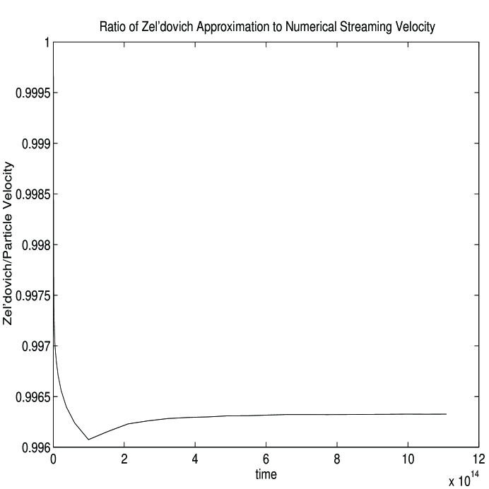
Figure 1: A plot of the ratio of the analytical infall velocity to the numerical result. After an initial correction, the infall velocity is correct to $\%0.4$.

As mentioned above, the analytical result for the ‘second turnaround’ is exact until just after the point where a particle crosses the path of another particle. In figure 2, we plot the analytical result versus particle trajectories. The discrepancy can be seen once the particle falls back toward the symmetry axis. It is interesting to note that the wake width does not grow as $t^{2/3}$ until after ‘binding’ occurs. The solution follows a transient from the formation stage to the growing stage, resulting in a smaller wake than would be predicted if one assumed the onset of self-similarity directly after the first particle falls back toward the symmetry plane. We also plot the growth ($\sim a(t)$) given in equation 12 from the point where this second stage in the evolution of the wake takes over. In figure 3 we plot the second turnaround radii (analytical and numerical) for the evolution of the wake until late times. The analytical curve matches well with the numerical wake radius relatively quickly (notice that the plot axes are logarithmic). If we extrapolate the curve to time $t_{0}$, we find a wake size of about $2x_{turn}=0.55h_{50}^{-1}Mpc$ for $z_{i}=10000$ and $v_{s}=0.5$.

Figure 2: A plot of the trajectories of a number of particles compared with analytical results. In the first stage of growth of the wake the leading particle’s trajectory is enveloped by the analytical trajectory for a particle being kicked away from the symmetry axis. In the second stage, where particle turnaround grows as $a(t)$, the turnaround radius is enveloped by the analytical $t^{2/3}$ power law. In this figure, solid curves with $+$ signs indicate analytical results, other solid curves are numerical results.

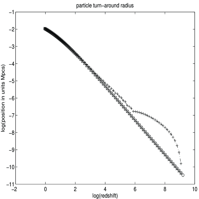
Figure 3: Here, particle turnaround (ie. the width of the wake) (dash-dot line with plus signs) is plotted versus the analytically calculated growth law (solid line with circles and crosses) well into the evolution of the wake. Note the close correspondance over the final $3$ orders of magnitude in redshift.

In figures 4 and 5, we plot the phase space of the particles in a cold dark matter simulation with $z_{i}=10000$ and $v_{i}=0.5c$. The velocity axis scales as $a^{-1/2}$ and the position axis scales as $a(t)$ in order to make the self-similarity evident. The phase space is similar to that shown in Fillmore and Goldreich [15] in their figure 2. The main difference comes from the velocities outside the non-linear region. In the phase space of a cosmic string wake, the streaming velocity outside the non-linear region is constant. This is because the velocity perturbation from the string is due to the conical deficit angle which extends approximately to the Hubble radius. Thus, in the Newtonian approximation, all particles have the same velocity, regardless of distance from the symmetry axis.

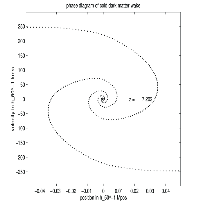
Figure 4: A plot at a late time ($z=7.202$) of the particle phase space of a cold dark matter wake formed at $z_{i}=10000$ with $v_{kick}=0.5c$. Each turnaround in the phase space trajectory corresponds to a peak in the wake overdensity.

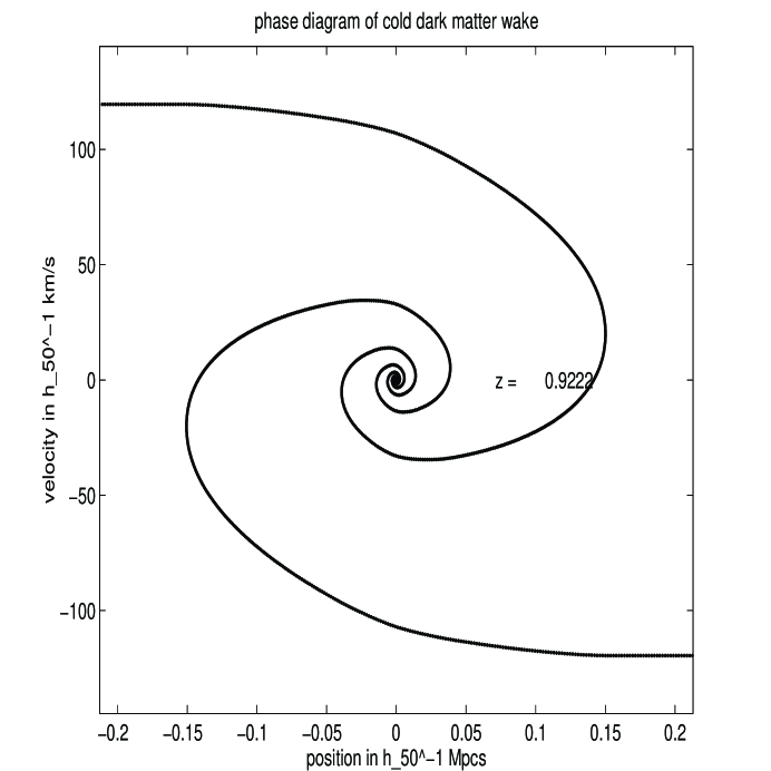
Figure 5: A plot at a late time ($z=0.922$) of the particle phase space of a cold dark matter wake formed at $z_{i}=10000$ with $v_{kick}=0.5c$. Notice the self-similarity with the previous figure.

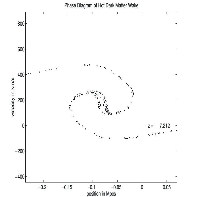
Figure 6: A plot at a late time ($z=7.212$) of the particle phase space of a hot dark matter wake formed at $z_{i}=10000$ with $v_{kick}=0.5c$. Each turnaround in the phase space trajectory corresponds to a peak in the wake overdensity. The position of only one in $512$ particles is plotted.

In figure 6, we plot the phase space of the particles in a hot dark matter simulation with $z_{i}=10000$ and $v_{i}=0.5c$. The phase space looks similar (except for a certain raggedness, which is from shot noise) to that of the cold dark matter wake at late times. In simulations, we find that accretion does not begin until the free-streaming length is smaller than the width of the wake. Before this time, the effective pressure of the neutrino gas keeps structure from forming on small scales.

The neutrino free-streaming length grows until $t_{eq}$, then decays as $a(t)^{-1/2}$. We can approximately calculate the time when wakes formed at $t_{eq}$ should begin to accrete by finding the time when the particle turnaround (calculated above for cold dark matter) is equal to the free-streaming length. This calculation gives a result

$$t_{accrete}\simeq 4.5\times 10^{24}\frac{1}{bv_{kick}}\bigg{(}\frac{bt_{eq}}{t_{0}}\bigg{)}.$$ (14)

Thus, accretion should begin at $z_{accrete}\sim 30$.

Numerically, we define a wake to be accreting once the overdensity $\delta\rho/\rho=1$. We find hot wakes formed at $t_{eq}$ beginning to accrete in our numerical simulations at $z_{accrete}\simeq 30$ and second turnaround achieved at $z_{turn}\simeq 8$. After second turnaround the phase space of hot wakes resembles that of cold wakes with the overdensity rapidly becoming self-similar and growing roughly as $a(t)$. We cannot make more quantitative statements due to the growth of spurious perturbations from statistical fluctuations in the initial conditions. However, after the onset of accretion in hot dark matter wakes, the evolution proceeds much as it would for cold dark matter with a rapid approach to self-similarity.

5 Discussion and Conclusions

In this work, we have presented results from a high-resolution numerical simulation of the evolution of the hot and cold dark matter distribution in cosmic string wakes. We have also extended the Zel’dovich approximation and found expressions for the size of the dark matter overdensity in wakes. We have compared these and previous results derived using the Zel’dovich approximation to our numerical results and find good agreement.

The most massive wakes today are those that have the longest time to accrete. These wakes are formed at $t_{eq}$. Our simulations give a wake width of $1.17h_{50}^{-1}Mpc$ for wakes formed at $z_{eq}$. Hot dark matter wakes are kept from accreting until the mean free path of the neutrinos falls below the size scale of the wake. The redshift that this occurs for a wake formed at $t_{eq}$ with $v_{kick}=0.5c$ is $z_{accrete}\sim 30$. We find good agreement with this prediction in our hot dark matter simulations, with accretion beginning at the time calculated from rough arguments.

In a cold dark matter wake, our results show two distinct stages of behavior of the wake width: the first stage is a brief epoch of essentially linear growth and contraction immediately following wake formation, and a second stage in which the overdensity begins to grow as particles accrete onto the wake. The transition between the linear stage and the growing stage is an interesting non-linear phenomenon. The fast approach to non-linearity makes the cosmic string wake a useful testbed for n-body codes.

To get an understanding of the cosmological implications of these results, we use data from network simulations. Cosmic string velocities from simulations are distributed with a broad peak in the distribution at about $v_{s}=0.3$ on horizon scales. Thus, the average cold string wake formed at time $t_{eq}$ will form a wake of mass $3.2\times 10^{-8}$ of the mass in the horizon at $t_{0}$. Combined with network simulation results (mentioned above) that there are $\sim 10-30$ strings per horizon volume, all of the matter in a cold dark matter universe would be non-linearly accreted at present. Some caveats to this result are that our simulations assume a matter dominated universe, and that coarse-graining in network simulations may lead to an incorrect estimate of the number of strings per horizon [16]. Nevertheless, a significant fraction $\sim 1/6$ of the matter in the universe would still be non-linear even if there were only $\sim 1$ string per horizon.

In the analogous hot dark matter universe, significantly less matter will be non-linear due to the late accretion time for hot wakes. Hot wakes formed at $t_{eq}$ by cosmic strings with velocities $v\sim 0.5c$ begin to accrete at $z\sim 30$. Early structure formation is therefore not a problem in the HDM plus cosmic string model (strings with higher velocities will form wakes that accrete even earlier). If we use the cold dark matter expressions for wakes forming at this redshift, we find that a fraction $0.002$ of the matter in the universe is in hot wakes. This fraction will go up if we integrate over all wakes. Also, recent work on the string network scaling solution shows that the length in long strings is roughly two orders of magnitude higher in the radiation era than in the matter era ${}^{\cite[cite]{[\@@bibref{}{wakescale}{}{}]}}$. This work shows that there is a relatively long transition between the two scaling regimes, and thus, there will be more long strings than previously thought around $t_{eq}$. This effect will again push the amount of accreted matter upwards.

6 Acknowledgements

I would like to thank R. Brandenberger for helpful discussions. This work has been supported by UK PPARC grant GR/K29272.

References

- [1] M. Rees, Mon. Not. R. Astr. Soc. 222, 27p (1986)
- [2] P.P. Avelino & E.P.S. Shellard, Phys. Rev. D51, 369 (1995)
- [3] A. Sornborger, R. Brandenberger, B. Fryxell & K. Olson, accepted Ap. J., for publication June 10, 1997.
- [4] A. Albrech & A. Stebbins, Phys. Rev. D 68, 2615 (1992)
- [5] A. Vilenkin, Phys. Rev. Lett. 46, 1169 (1981)
- [6] A. Albrecht & N. Turok, Phys. Rev. D40, 973 (1989)
- [7] D. Bennett & F. Bouchet, Phys. Rev. Lett.60, 257 (1988)
- [8] B. Allen & E. P. S. Shellard, Phys. Rev. Lett.64, 119 (1990)
- [9] A. Vilenkin, Phys. Rev. D23, 852 (1981)
- [10] J. Gott, Ap. J.288, 422 (1985)
- [11] T. Vachaspati & A. Vilenkin, Phys. Rev. Lett.67, 1057 (1991)
- [12] L. Perivolaropoulos, R. Brandenberger & A. Stebbins, Phys. Rev. D 41, 1764 (1990)
- [13] A. Stebbins, S. Veeraraghavan, R. Brandenberger, J. Silk & N. Turok, Ap. J. 322, 1 (1987)
- [14] R. Hockney & J. Eastwood, Computer Simulation Using Particles, Adam Hilger (1988)
- [15] J. Fillmore & P. Goldreich, Ap. J. 281, 1 (1984)
- [16] B. Carter, Phys. Rev. D 41, 3869 (1990)
- [17] C. Martins & E.P.S. Shellard, Phys. Rev. D 54, 2535 (1996)