Evolution of a hot primordial gas in the presence of an ionizing ultraviolet background: instabilities, bifurcations, and the formation of Lyman limit systems

Abstract

The time evolution of thermal and thermo-reactive instabilities of primordial gas in the presence of ionizing UV radiation is studied. We obtain conditions (depending on density, temperature, and UV radiation intensity) favorable for the formation of a multi-component medium. Nonlinear effects, especially those attributable to opacity, can play an important role. In certain parameter regimes, dramatic, rapid evolution of ionization states away from ionization equilibrium may occur even if system control parameters evolve slowly and the system starts in or near ionization equilibrium. Mathematically, these rapid changes may best be understood as manifestations of bifurcations in the solution surface corresponding to ionization equilibrium. The astrophysical significance of these instabilities is that they constitute a nongravitational mechanism (thermo-reactive instability) for decoupling isolated spatial regions with moderate initial fluctuations from their surroundings, even under the influence of heating processes due to ionizing UV radiation. In particular, isolated, decoupled regions with relatively high neutral hydrogen density may result, and these could be associated with Lyman alpha clouds of high column density or with Lyman limit systems.

1 Introduction

An understanding of processes occurring in diffuse gas interacting with a photoionizing flux is of direct importance in modeling a number of astrophysical phenomena, such as quasar absorption clouds (Doroshkevich, Mücket, and Müller, 1990; Ferrara & Giallongo, 1996) and the structure of neutral hydrogen clouds in galactic halos (Ferrara & Field, 1994). The effects of heating due to photoionization in galaxy formation have been considered by Efstathiou (1992) in the context of mechanisms for suppression of dwarf galaxy formation and by Navarro and Steinmetz (1996) in their study of the “overcooling” problem. These authors found that photoionization alone could not provide the heating mechanism required, i.e., supernova feedback should also be included. Cosmological simulations of galaxy formation including star formation and supernova feedback have been carried out by Yepes, Kates, Klypin, & Khokhlov (1996; hereafter YKKK). A reasonable hypothesis is that photoheating indirectly influences star formation by regulating the conditions for thermal instability and thus the formation of a multiphase (cloudy) medium.

Since many of the observable phenomena involving photoionization require a prediction of statistical properties of objects, it is important to integrate the local dynamics of diffuse gas (i.e., heating, cooling, ionization, formation of neutral hydrogen) into an overall approach including hydrodynamics and the evolution of large-scale structure. As these processes involve a large dynamical range of scales, some of them will inevitably occur below the limits of resolution of a numerical simulation. Due to the presence of nonlinearities, the effects of fluctuations below a typical cell size will require special attention, especially when instabilities are involved.

It has long been appreciated (Field 1965; Defouw 1970; Balbus 1986; Fall & Rees; 1985; Ibañez & Parravano 1982) that gas subject to cooling (and perhaps heating) processes in a cosmological setting may become thermally unstable, leading to enhanced cooling and the formation of a multiphase medium including cool clouds (Begelman & McKee, 1990). Cool clouds play an important role in theories of the interstellar medium (McKee & Ostriker, 1977) and galaxy dynamics, due to their effects on the energy budget (enhanced cooling), star formation and ”supernova feedback” (YKKK).

Corbelli & Ferrara (1995) have demonstrated the existence of so-called ”thermo-reactive” instability modes for gas containing metals in the presence of ionizing radiation. Here we will see that instabilities of thermo-reactive type are also possible in gas of primordial composition. In particular, our results imply that thermo-reactive instabilities could play an important role in the formation of at least some population of observed Lyman limit systems.

The principal goal of this paper is to study the dynamics of fluctuations in a gas of primordial composition which may already have been compressed to high ambient density (compared to the background density of the universe) and heated to high temperature as a consequence of large-scale structure formation. The intention is to characterize instability regimes approximately as a function of the ambient temperature and density of the gas, with local effects of gravitation excluded. Such a characterization is expected to be useful for an understanding of conditions for star formation in the context of hydrodynamical numerical simulations. For this application, linear instability analysis about ionization equilibrium solutions does not tell the whole story: For one thing, even if present, some linear instability modes are too slow to be of importance on a dynamical timescale. Moreover, some of the instabilities which occur involve nonlinearity in an essential way and could not be detected by linear analysis. (Because opacity is involved, the strength of the nonlinear effects increases with the size of the perturbed region; see also Ferrara and Field (1994).)

Apart from its importance for the intended applications, the nonlinear system studied in this paper is quite interesting from a purely mathematical point of view: As seen here [and as previously pointed out for example by Petitjean, Bergeron, and Puget (1992)], the equations of ionization equilibrium exhibit multivalued solutions in certain regimes of parameter space. We propose that these solutions are best understood in terms of the theory of bifurcations (or catastrophes): Bifurcations are typical in the equilibria of nonlinear systems, and the mathematical theory (see for example Arnol’d, 1979; Chow & Hale, 1985) gives strong hints and indications of the general behavior to be expected. Near bifurcations, a system can depart rapidly from equilibrium even if the control parameters vary slowly. (In the present case, the “slowly-varying” control parameters are any two thermodynamic variables, say temperature and – on a still longer time scale – pressure.) Hence, even a qualitative understanding of system evolution near bifurcations requires a time - dependent treatment of the coupled system of ionization, heating, and cooling equations. The importance of simulating the dynamical equations for evolution of ionization states was previously discussed for example by Cen (1992), and a dynamical treatment has been incorporated into the hydrodynamic code used in a number of papers (Cen et al. 1990,1992,1993,1994). However, for numerical efficiency it would be useful to know under what circumstances ionization equilibrium is in fact a good approximation.

The organization of this paper is as follows: Section 2 gives the model system of equations describing the dynamics of the three species H_I, He_I, and He_II for a gas of primordial composition. Section 3 shows that the solution manifold of the ionization equilibrium equations can exhibit the properties of a mathematical bifurcation surface (Golubitsky & Schaeffer, 1985). Of special interest are the solution trajectories of constant pressure, for which one sees that evolution through equilibrium solutions is not always possible. Section 4 considers selected solutions of the full time-dependent equations exhibiting some typical behavior. Section 5 characterizes the regimes of temperature and density in which instabilities relevant to numerical simulations (i.e., those with sufficiently short timescales) are most likely to occur. Section 6 summarizes and describes in particular some potentially interesting implications for Lyman limit systems.

2 Equations describing thermal and ionization evolution

Consider first the time-evolution of a sufficiently small region such that the density $\rho(t)$ and gas temperature $T(t)$ may be treated as approximately uniform. (This approximation will be discussed below in connection with the optical depth $\tau_{\nu}$.) Self-gravity is neglected. The dynamics in this region are assumed to depend on Hubble expansion, cooling processes, and heating due to a UV background. The UV background is assumed to be described by an externally generated, explicitly time-dependent, spatially uniform flux $J(t)$.

We restrict our consideration to a region containing hot gas with primordial abundances, i.e. the total helium number density $n_{He}$ is 10 % of the total hydrogen number density $n_{H}$. The medium is characterized in addition by the number densities $n_{HI}$,$n_{HII}$,$n_{HeI}$,$n_{HeII}$ and $n_{HeIII}$ of its ionization states HI, HII, HeI, HeII, and HeIII, respectively. One also has $n_{H}=n_{HI}+n_{HII}$ and $n_{He}=n_{HeI}+n_{HeII}+n_{HeIII}$ and the equations of charge conservation.

The evolution of these number densities is determined by the equations

$${dn_{HI}\over dt}=-\xi_{HI}n_{HI}-\xi_{e,HI}n_{HI}n_{e}+n_{HII}n_{e}\alpha(HII)$$ (1)

$${dn_{HeI}\over dt} = -\xi_{HeI}n_{HeI}-\xi_{e,HeI}n_{HeI}n_{e}$$ (2)

$$+n_{HeII}n_{e}\alpha(HeII)$$

$${dn_{HeII}\over dt} = -\xi_{HeII}n_{HeII}-\xi_{e,HeII}n_{HeII}n_{e}$$ (3)

$$+n_{HeIII}n_{e}\alpha(HeIII)-{dn_{HeI}\over dt}$$

In the above equations, $\xi_{i}$ and $\xi_{e,i}$ [with $i$ ranging over (HI,HeI, HeII)] denote the rates of photo- and collisional ionization, respectively, $n_{e}$ and $n_{i}$ are the electronic and ionic number densities, and $\alpha(i)$ denotes the recombination rate from species $i$ to the next lower ionization state. The photo-ionization rate $\xi_{i}$ for the $i$-th species is written in the form

$$\xi_{i}(x)=\int_{\nu i}^{\infty}4\pi{J_{\nu}(x)\sigma_{i}(\nu)\over h\nu}d\nu$$ (4)

where the $\nu_{i}$ are the threshold frequencies of each species, $J_{\nu}$ is the intensity of the diffuse background UV flux in units of ergs s^-1 cm^-2 Hz^-1 sr^-1, and $\sigma_{i}(\nu)$ is the photoionization cross section, which is approximated using the expressions given by Kramers (1923).

In addition to the primary ionizations described by Eq. (4), secondary ionizations could contribute to the number density evolution (Shull, 1979; Shull & van Steenberg, 1985; Ferrara & Field 1994). However, there is observational evidence for a steepening of the UV spectrum at the HeII edge (Jakobsen et al., 1994; Ferrara & Gialongo, 1996). Hence, the energy of most secondaries will be low enough that a large fraction, though not all, of the energy will be converted to heat.

The diffuse flux is diminished by absorption due to surrounding gas layers (self-shielding). The optical depth at a distance $x$ from the surface is given by

$$\tau_{\nu}=\int_{0}^{x}dx^{\prime}\sum_{i}n_{i}(x^{\prime})\sigma_{\nu}(i)$$ (5)

where in the summation $i$ ranges over all three species for $\nu_{\rm HeII}\leq\nu$, over HeI and HI for $\nu_{\rm HeI}\leq\nu<\nu_{\rm HeII}$ and over HI for $\nu_{\rm HI}\leq\nu<\nu_{\rm HeI}$.

We model the UV flux in Eq. (4) as a power law spectrum with spectral index $\alpha$; it may thus be expressed in the form

$$J_{\nu}(x)=J_{0}(\nu/\nu_{LL})^{-\alpha}\exp(-\tau_{\nu}(x))$$ (6)

where $J_{0}$ is the intensity at the Lyman limit; we take $\alpha=1$ in the calculations that follow.

For later use, it will be convenient to introduce a shielding depth for HI defined by

$$\tau_{HI}\equiv-\log(\xi_{HI}/({4\over 3}\pi J_{0}G^{B}_{HI})),$$ (7)

where $G^{B}_{HI}$ is the parameter calculated by Black (1981) for the optically thin case. (Shielding depths for HeI and HeII can be defined similarly.)

A knowledge of the above quantities allows us to obtain the heating rates by photoionization

$$\Gamma_{i}(x)=\int_{\nu i}^{\infty}4\pi{J_{\nu}(x)h(\nu-\nu_{i})\over h\nu}\sigma_{i}(\nu)d\nu$$ (8)

and to construct the total heating rate

$$\Gamma=\sum_{i}\Gamma_{i}n_{i}.$$ (9)

The cooling rate $\Lambda$ is calculated according to Black (1981), and Compton cooling is included.

Now, the flux $J_{\nu}$ appearing in the photoionization rates (4) and the heating rates (8) is a monotonically decreasing function of $x$, which differs from an exponential because of the $x$-dependence of $\tau_{\nu}$, which itself depends on the $n_{i}(x)$. As we will see below, even in a region with moderate gradients and slowly evolving thermodynamic state variables (pressure and temperature) the number densities $n_{i}$ of the ionization states can have large gradients and can also change rapidly. Nonetheless, because the $x$ - dependence of (4) and (8) is the same, one may always define weighted means $n_{i}$ such that the integral in Eq. (5) is replaced by

$$\tau_{\nu}=x\sum_{i}n_{i}\sigma_{\nu}(i)$$ (10)

where the summation is as above and Eqs. (4) and (8) remain accurate as written. Of course, these weighted means $n_{i}$ still depend on $x$, and they are not strictly equal to the average number densities.

Here we identify the true average number densities with these weighted values and use them in the evolution equations (1), (2), (3). For the optically thin case, this is an excellent approximation, whereas in the optically thick case there are some quantitative (but not qualitative) inaccuracies as discussed in the Conclusions.

3 Bifurcation structure in the manifold of solutions for ionization equilibrium

One can gain some insight into the time-dependent problem by studying the system representing ionization equilibrium, which is obtained by setting all time derivatives to zero in Eqs. (1), (2) and (3). (For the purposes of this discussion, the environment is considered static, i.e., constant flux intensity $J_{0}$, no cosmological expansion.) For a range of number densities $n_{H}$ and temperatures $T$, the complete set of possible solutions for $n_{HI},n_{HeI}$ and $n_{HeII}$ was identified and found numerically. Each solution corresponds to some net heating (or cooling) rate $\Gamma-\Lambda\propto\dot{T}\equiv dT/dt$, and the locus of equilibrium solutions defines a two-dimensional surface embedded in a three-dimensional space with coordinates ($n_{H}$, $T$, $\Gamma-\Lambda$).

Fig. 1 shows a plot of this surface in the range $10^{-4}cm^{-3}<n_{H}<2\times 10^{-3}cm^{-3}$ and $1<T_{4}<5$, where $T_{4}$ is the temperature in units of $10^{4}$K. The flux intensity was $J_{0}=$ $J_{21}$ $10^{-21}$ ergs s^-1 cm^-2 Hz^-1 sr^-1, with $J_{21}\approx 0.05$. This flux density provides a typical example of a surface containing a classical catastrophe or bifurcation fold which appears to terminate in one or more cusps of the generic type described by Whitney (1955): For temperatures near $1.3<T_{4}<2.1$ (the precise range depending on the density within the regime $5\times 10^{-4}<n_{H}<10^{-3}$) there are three solutions for a given $n_{H}$, $T$.

The existence of a bifurcation has profound consequences. First, as a general property, any system is essentially nonlinear near a bifurcation, and therefore there is no hope of understanding the resulting instabilities from a linearized analysis. Secondly, as control parameters of a (time-dependent) system initially in a state of equilibrium are slowly varied, departures from equilibrium are path dependent: if the path passes through a region with no folds, the system may evolve quasistatically through a family of nearly ionization equilibrium states. However, near a bifurcation even a slow change in control parameters forces the system to undergo such rapid evolution that time-dependent solutions would be expected to depart substantially from (ionization) equilibrium.

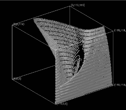
Figure 1: 3-dimensional surface plot of $[\Gamma-\Lambda]$ as a function of $n_{H}$ and $T$ in the range $10^{-4}cm^{-3}<n_{H}<2\times 10^{-3}cm^{-3}$ and $1<T_{4}<5$. The surface is folded and contains at least one bifurcation (axes as indicated in the lower panel).

For a qualitative illustration of what to expect from time dependent simulations and for further understanding of the bifurcations, it is useful to study the behavior of $\dot{T}=dT/dt$ (or equivalently $\Gamma-\Lambda$) along curves of constant pressure $P$ but changing $T$. The isobaric trajectories define a one-parameter family of hyperbolae through the two-dimensional ($n_{H}$, $T$) parameter space. The time-evolution of $n_{H}$ and $T$ for this restricted system corresponds to moving along one of these hyperbolae either in the direction of decreasing $T$ (cooling) or increasing $T$ (heating) at the rate given by $\dot{T}$.

Fig. 2 shows a family of plots of $\Gamma-\Lambda$ vs. $T$ along hyperbolae defined by $P$=const for varying flux coefficients (from top (1) to bottom (4)) $J_{21}$=[0.05, 0.01, 0.005, 0.001]. As the flux decreases, the curves have deeper minima. Beginning on the left, as long as $\Gamma-\Lambda<0$, an isobaric system would move along the curve to the right (decreasing temperature). For the low-flux curve (4), the temperature drops monotonically until thermal equilibrium is reached somewhere below $10^{3}$ K. The only other noteworthy feature in this temperature range is a higher cooling rate near $T_{4}=1.7$.

Figure 2: Energy loss ($\Gamma-\Lambda$) for different UV fluxes at constant pressure $n_{H}T=0.95\cdot 10^{2}$ K cm^-3.

Figure 3: Energy loss ($\Gamma-\Lambda)$ for various constant pressures and constant UV flux $J_{21}$ = 0.01. Curve (1): $P$ corresponds to $T_{4}=0.95$ at $n_{H}=10^{-3}$; Curve (2): $P=$ 5 times higher than curve (1) Curve (3): $P=$ 10 times higher than curve (1) Curve (4): $P=$ 50 times higher than curve (1)

The next higher flux ($J_{21}$=0.005) curve (3) is triple valued between $T_{4}=1.7$ and the cusp near $T_{4}=1.6$. The three solutions correspond to three different ionization states solving the equilibrium equations. With respect to the full time-dependent equations, the two solutions with the highest and lowest values of $n_{HI}$ are stable (attractive), while the middle solution is unstable (repulsive). Moreover, this regime is likely to be reached by a time-dependent system, because $dT/dt$ is negative up to the cusp.

The next higher flux curve (2) also has a triple-valued regime, but the curve crosses the $T$ axis (thermal equilibrium) near $T=1.4$ and thus is not forced to the cusp. Nevertheless, three solutions of the ionization equilibrium equations are available in the range where the system is still cooling. If some perturbation (such as a small variation in the flux or external pressure) occurs, it is possible for the system to jump to the lower stable solution, cool, and evolve to lower temperatures.

The upper curve in Fig. 2 includes a triple-valued solution within the heating regime (see upper right). A system initially at $T_{4}<1$ would be heated until reaching the cusp near $T_{4}=1$ and could then jump to the lower branch with a lower heating rate.

The curves in Fig. 3 are similar to those of Fig. 2, except that the pressure is varied for constant flux. In the lower curve (4), the solutions are single-valued and do not enter the heating regime. The next higher curve (3) has a very steep gradient near $T_{4}=2.0$, where it passes rather close by the bifurcation. The next curve (2) is analogous to curve (3) in Fig. 2. Following the upper curve (1) from left to right, a system at strictly constant pressure would stabilize near $T_{4}=2$ before the multi-valued region is reached. However, slight departures from constant pressure could move the system to the multi-valued region and permit a rapid change to the other stable branch.

The behavior of the curves in Figs. 2 and 3 is quite typical of systems with a bifurcation. In particular, they illustrate the difficulties likely to arise in a numerical simulation.

For all of the multi-valued curves of Figs. 2 and 3, the solution with the largest cooling rate is also associated with a drastically higher fraction of neutral hydrogen. In particular, at a given pressure it is possible for the system to have both an optically thin and an optically thick stable state. This possibility gives a hint that there could be structures associated with the existence of qualitatively different phases in neighboring regions with initially similar (but not identical) control parameters.

4 Evolution and instability of perturbed regions in an ambient hot primordial gas

In the previous section, we saw that an isobaric system may cool in such a way that it is forced out of ionization equilibrium. Moreover, we wish to study the evolution of a system evolving so quickly that the control parameters $T$ and $n_{H}$ need not change simply quasistatically, because the timescales associated with cooling and/or expansion may be short compared to the relaxation time to ionization equilibrium. Both of these problems require solution of the time-dependent equations (1 - 3).

Figure 4: Evolution of characteristic parameters as a function of the redshift $z$ for initial conditions $z_{i}=4$, $T_{h}=20$, $n_{h}=0.75\times 10^{-3}$ cm^-3, $J_{21}(z_{i})=0.5$. (The flux $J_{21}(z)$ evolves according to Fig. 10.) Starting from the lower left of the figure: Two bottom lines: shielding depth $\tau_{HI}$ (definition see Eq. (7) for the hot (1; dot-dot-dot-dash) and cold (2; dot-dash) components. Long dashed curve (3): ratio (hot-to-cold) of Jeans lengths. Solid curve (4): $-\log_{10}(n_{HI}/{\rm cm}^{-3})$ for the cold component. Dotted curve (5): $T_{c}$ in units of $T_{4}$. Short dashed line (6): $T_{h}$ in units of $T_{4}$.

Figure 5: Evolution as in Fig. 4, except that the density is increased by a factor of 2. Labeling as in Fig. 4.

Figure 6: Evolution as in Fig. 5, except that the initial flux is reduced by a factor of 10 to $J_{21}=0.05$. Labeling as in Fig. 4.

We are interested in the evolution of structures in the intergalactic medium and particularly in the formation of cold clouds. These effects may occur in a variety of environments, including both gas which is still comoving with the Hubble flow and gas in structures that have decoupled from the expansion. In this paper, we derive results for the former case (comoving); however, as discussed below, the effect of decoupling the gas from the expansion would usually tend to enhance the effects studied here.

In general, the equations of cooling and ionization are coupled to the gas dynamical equations, as well as to gravitation. However, the qualitative character of the instabilities can be studied without the full generality of gas dynamics. The ”one-cell” dynamics considered here could be generalized to include advection within the context of a numerical simulation that does include gas dynamics and gravitation (see for example YKKK).

We consider a gas with primordial composition consisting of two components:

• an ambient (“hot”) component at temperature $T_{h}(t)$, with uniform number density $n_{h}$ (not to be confused with $n_{H}$, the hydrogen density). The gas is assumed as explained above to be comoving with the cosmic expansion.

• an initial perturbation (the “cold” component) consisting of a slightly compressed region with number density $n_{c}$ (assumed spatially constant in the perturbed region) evolving in pressure equilibrium with the hot component and therefore at a lower temperature $T_{c}=T_{h}n_{h}/n_{c}$. For concreteness, we consider the cold perturbation region to be a flat slab of thickness $50$ kpc. However, subject to the approximation of Eq. (10), the results should apply to a range of geometries.

We take a ratio of baryons to dark matter of $\Omega_{B}=0.1$ in both components and ambient density contrast $\delta$ initially with respect to an assumed background number density of $2\times 10^{-7}$ cm${}^{-3}(1+z_{i})^{3}$. This implies $n_{h}$ is initially $(2\times 10^{-7}$ cm${}^{-3})(1+z_{i})^{3}(1+\delta)$.

In many treatments of thermal instability such as Fall & Rees (1985), Field (1965), one is primarily interested in whether or not a perturbation can decouple. Here, decoupling is only of interest if it occurs on a time scale short compared to $t_{\rm grav}\propto t_{\rm Hubble}/\sqrt{(}1+\delta)$.

Suppose that the gas is initially in ionization equilibrium. Assuming an initial perturbation of $10\%$ at some initial redshift $z_{i}$, we study instabilities by following the evolution during the time $t_{\rm grav}$. During the evolution we monitor parameters characterizing possible decoupling of the system including

• the ratio $\rho_{c}/\rho_{h}$

• the temperatures $T_{c}$ and $T_{h}$

• the fractions $n_{HI}$ of neutral hydrogen

• the optical depths $\tau_{c}$ and $\tau_{h}$

• the ”cooling enhancement” ratio $E_{c}/E_{h}$, where for each component $E$ is the energy lost (gained) per unit volume

• the multiplicity of the solutions of ionization equilibrium, if applicable

• the Jeans lengths for each component

As disussed by Cen (1992) in a more general context, an important technical problem is the presence of several varying time scales, including $t_{\rm grav}$, the cooling times $t_{\rm cool}$, and the various time scales associated with the time-dependence of the three species $n_{HI}$, $n_{HeI}$, and $n_{HeII}$ in Eqs. (1 - 3). The complete time dependent equations are solved at all times using adaptive timestep control taking into account the shortest relevant timescale. However, it sometimes occurs that the time-dependent solution is close to an (ionization) equilibrium solution. It is then computationally efficient to use a different algorithm which finds an appropriate equilibrium solution and tests that this solution is indeed close to the time-dependent solution sought. In this case, the timestep is comparable to the dynamical time scale $t_{\rm dyn}$, the minimum of $t_{\rm grav}$ and $t_{\rm cool}$.

Fig. 4 shows the evolution with redshift of characteristic parameters for initial conditions $z_{i}=4$, $T_{h}=20$, $n_{h}=0.75\times 10^{-3}$ cm^-3, $J_{21}=0.5$. This density corresponds to 30 times the background density. For these parameters, no thermo-reactive instability occurs during a time $>>t_{grav}$ ( $t_{grav}\approx 10^{8}$ years), and the cold component does not decouple from the environment: The shielding depths $\tau_{HI}$ for the hot and cold components coincide in the figure. Both components remain optically thin throughout. The curve (3) giving the ratio of the Jeans length of the hot component to that of the cold component attains a value of about 5 during the course of the simulation and has flattened out considerably by the end of the simulation at $z=1.9$. Neither component has become Jeans unstable within the time scale considered.

Fig. 5 is for the same parameters as in Fig. 4, except that the density is increased by a factor of 2. This figure illustrates how an instability may indeed be present (i.e., according to linear perturbation theory) whose timescale for decoupling however is longer than the dynamical timescale. Clearly, some degree of decoupling has taken place: the ratio of Jeans lengths (hot to cold) is 10 and still growing, and $T_{h}$ is about 4 times $T_{c}$. As before, the shielding depths $\tau_{HI}$ for the hot and cold components are practically indistinguishable.

In contrast to the above two figures, Fig. 6 shows a clear case of decoupling. The parameters are as in Fig. 5, except that the initial flux has been reduced by a factor of 10 to $J_{21}=0.05$. Even in this case the optical depths of the cold and hot component remain very close until about $z=3.77$. However, subsequently, the optical depth of the hot component barely changes, remaining optically thin as in Figs. 4 and 5, whereas the cold perturbation becomes optically thick ($n_{HI}$ increases by more than four orders of magnitude) and at the same time rapidly cools and thus drastically decreases its Jeans length, until it becomes gravitationally unstable. Note that the rapid increase in neutral hydrogen density at $z=3.75$ is not a numerical artifact, but represent rapid evolution as in Figs. 2 and 3 where the solutions of the static ionization equilibrium equations are multi - valued. This evolution provides an example of nonlinear thermo-reactive instability and results in a strong decoupling of the cold perturbation from its environment.

5 Investigation of instability regimes in the parameter space of density and temperature

As mentioned above, one important goal of this paper is to determine what regimes of ambient density and temperature are favorable for eventual star formation in a region containing primordial gas. The arguments given here apply to “star formation” as it occurs in the context of the McKee - Ostriker (1977) theory of the interstellar medium. Now, the formation and evolution of the interstellar medium are certainly complicated processes involving various modes of instability on a range of spatial and time scales. However, thermal or thermo-reactive instabilities are expected to be a necessary prerequisite for such a multiphase medium to arise in the first place. Hence, a characterization of those regimes of ambient gas temperature and density likely to produce thermo-reactive or thermal instabilities will give information on environments favorable for star formation. (Since instability depends on UV flux density as well as density and temperature, the flux will obviously play an important role in regulating star formation.)

To this end, we have simulated the evolution of “cold” and warm components in pressure equilibrium as in Section 4 under a wide range of initial conditions in number density and temperature, and also for a variety of realistic flux and redshift combinations. All simulations began with an initial gas density perturbation of 10 % and were continued until either the colder component cooled to below 5000 K or the local Hubble time $t_{\rm grav}$ defined above was exceeded. (Some perturbations which would be classified as “unstable” according to linear perturbation analysis would nonetheless fail to cool within this time.) The dimension of the perturbed region was taken to be $50/(1+z)$ kpc.

We now present detailed results of several simulations on a finely-spaced, two-parameter grid (temperature-number density). We first consider the case of initial redshift z=0.1 and flux $J_{21}=0.01$: Fig. 7 is a contour plot of the ratio ${\rho_{c}/\rho_{h}}$ evaluated at the end of the simulation. The horizontal axis is the initial temperature of the hot component in units of $10^{4}$ K, and the vertical axis represents the initial overdensity of the hot component (with respect to the mean gas density). The visible contours represent regimes in which the cold component actually did succeed in cooling. In the present discussion, we regard a final ratio ${\rho_{c}/\rho_{h}}>3$ as an indicator of decoupling (instability). Note that the density ratio could have been higher than its final value during the course of the simulation (see Fig. 5 near $z=3.75$). One may observe from the figure that the regime of instability as characterized by this indicator consists of the region roughly defined by the inequalities $T_{4}\geq 10$ (a vertical boundary) and

$$n_{\rm gas,init}>(400+25T_{4})n_{\rm gas,0},$$ (11)

where $n_{\rm gas,0}\approx 2\cdot 10^{-7}$ cm^-3 is the average gas density today.

Fig. 8 is a contour plot of the “enhancement” ratio of the cold to the hot component (ratio of total integrated heat lost per unit mass during the simulation for the respective components) for the same simulations as in Fig. 7. Again, although the final enhancement ratio may be lower than the maximum during the course of the simulation, it still may be regarded as an indicator of instability and decoupling. The regime of decoupling as defined by this indicator (enhancement greater than 1.5) in Fig. 8 coincides quite well with that defined by the final density ratio (Fig. 7). Again, the visible contours are plotted only if the perturbed gas actually cooled.

Since the UV flux changes with redshift, the instability regimes and thus the conditions for development of a multicomponent medium will evolve. Hence, one cannot necessarily estimate instability conditions in the distant past simply by extrapolating the low-redshift results to take into account the higher background density. We next report the results of higher-redshift simulations performed as before on a fine-parameter grid, but for the following redshift-flux combinations:

$z_{i}=3,J_{21}=0.1$ (see Fig. 9) and
$z_{i}=4$, $J_{21}=0.5$ and $J_{21}=1.0$.

These fluxes are all within the constraints provided by observations and large-scale structure simulations (Mücket et al., 1996; Bechtold, 1994; Williger et al., 1994; Bajtlik, Duncan, & Ostriker, 1988; Lu, Wolfe, & Turnshek, 1991; Haardt & Madau, 1995). It is quite remarkable that for these higher initial redshifts, the left (temperature) boundaries of the instability regimes are nearly unchanged from the low-redshift case and also hardly differ for the two flux values ($J_{21}$) considered: the temperature limit is still roughly characterized by $T_{4}>10$.

Figure 7: Contour plot of the ratio ${\rho_{c}/\rho_{h}}$ evaluated at the end of the simulation; initial redshift $z_{i}=0.1$ and initial flux $J_{21}=0.01$. Horizontal axis: $T_{4}$ for the hot component. Vertical axis: initial overdensity of hot component with respect to the background density. Contour labels: ${\rho_{c}/\rho_{h}}$

At redshift $z_{i}=3$ for an initial flux $J_{21}=0.1$, one can see from Fig. 9 that the bottom (density) boundary of the instability regime can be approximated by

$$n_{\rm gas,init}(z_{i}=3)>(25+1.8T_{4})*n_{\rm gas,0}\cdot(1+z_{i})^{3}.$$ (12)

At the initial redshift $z_{i}=4$ for the lower flux value (0.5), the regime of instability is roughly characterized by the condition

$$n_{\rm gas,init}(z_{i}=4)>(14+1.1T_{4})*n_{\rm gas,0}\cdot(1+z_{i})^{3}.$$ (13)

For the higher value ($J_{21}=1.0$), the lower density bound is shifted upward by an additional factor of about 1.3.

In order to investigate the general trend of evolution with redshift for the asymptotes described above, we have analyzed the instability behavior on a coarser grid with respect to ($T_{i},n_{H,i}$ ) for a sequence of redshifts $z_{i}=0.1,1,2,3,4,5$ and flux values $J_{21,i}$. As a model for the redshift dependence of the UV flux, we have used the results provided by simulations described in Mücket et al. (1996a) which reproduce the observations mentioned above quite well (see Fig. 10). The results are given in Table 1. For each initial redshift $z_{i}$, the asymptotes (as defined previously) are given approximately by an expression of the form

$$T_{4} = T_{0}=const,$$

$$n_{\rm gas,init}(z_{i}) = (n_{0}+m_{0}T_{4})*n_{\rm gas,0}\cdot(1+z_{i})^{3}$$ (14)

$z_{i}$ $J_{21}$ $T_{0}$ $n_{0}$ $m_{0}$ 0.1 0.008 12 400 5 1. 0.034 10 89 3 2. 0.061 8 44 1.75 3. 0.074 10 25 1.1 4. 0.073 10 17 0.65 5. 0.06 10 11 0.5

Table 1: The parameters $T_{0},n_{0},m_{0}$ for the asymptotes defining the regions of instability at given initial redshift $z_{i}$ and flux $J_{21,i}$ in the $n-T$ plane.

From these simulations, one may deduce that the parameter $n_{0}$ is most strongly determined by requiring that the flux be almost entirely shielded: Since we consider a planar slice of fixed comoving size $x_{0}=50$ kpc, this requirement would imply that the critical value $n_{0}$ is determined by the relation $\tau=x_{0}\sigma n_{HI}(1+z_{f})^{2}$, where $z_{f}$ is the redshift for which $n_{HI}\approx n_{0}n_{\rm gas,0}=n_{H}$, i.e., when hydrogen becomes neutral. The results of Table 1 roughly fit this relation for a critical optical depth on the order of $\tau\approx 10-15$ (taking into account typical differences between $z_{i}$ and $z_{f}$). The values $n_{0}(1+z_{i})^{2}$ in Table 1 vary within 20% around the value 400 (the scatter is probably attributable to the coarse computational grid of steps in $T$ and $n_{H}$ in the numerical calculations). There is also a weak (roughly logarithmic) dependence on the flux, as one would expect.

At higher temperatures ($T_{4}>10$) the terms describing collisional ionization become important. The stage at which the flux is shielded ($\tau\approx 10$) and cooling becomes strong enough is therefore shifted to higher densities $n_{H}$. Although the functional dependence is certainly more complicated, the slope $m_{0}(1+z)^{3}$ can be roughly estimated as being proportional to the flux $J_{21}$ up to redshift $z=4$.

We now return to the simulations discussed above for $z_{i}=0.1$ and $J_{21}=0.01$. In contrast to the decoupling criteria illustrated in Figs. 7,8, and 9, in which both cold and hot components always lost energy, in the low to moderate density contrast regime it is possible for decoupling to occur in which the hot gas component actually gains energy, while the cold perturbation loses energy (cools). This effect is seen in the contours of Fig. 11, which form a rough band in the figure. Above this band, there is a net energy loss in both components; below this band, there is a net energy gain in both components. The somewhat “speckled” behavior within the band is due to the fact that energy may be lost and gained within the course of a simulation. The existence of this band could be of great interest in a scenario in which the spatial dependence of shielding is treated more precisely than here. In this case, there could be a persistent core of opaque gas (high neutral hydrogen) surrounded by hotter, optically thin gas which is heated (See Ferrara & Field, 1994). Above the band, one would expect the core to increase gradually in size (as in a cooling flow), whereas below the band a perturbation might be expected to evaporate, especially if heat conduction is properly included.

In order to get an idea of the length scales of the structures involved, we apply the results of Cowie & McKee (1977) to the parameters considered here and obtain an expression for typical values of the critical evaporation timescale $t_{\rm evap}$, which involves the length scale. A critical evaporation length of 100 pc may then be estimated from the condition $t_{\rm evap}>t_{\rm cool}$. A larger limit is obtained from the condition $t_{\rm evap}>t_{\rm grav}$, which leads to a critical size of 1 kpc. This length scale also follows from a different line of argument given by Ostriker & Gnedin (1996).

Figure 8: Contour plot of enhancement (see text for definition); axes as in Fig. 7

Figure 9: Contour plot of the final value of the ratio $\rho_{c}/\rho_{h}$ as in Figs. 7, but for initial redshift z=3 and initial flux $J_{21}=0.1$

Figure 10: Log-log plot of redshift dependence of the UV flux obtained from N-body simulations; here the flux refers to $f=4\pi J_{21}$

Figure 11: Simulations as in Figs. 7 and 8: regimes in which hot gas gained net energy, but cold perturbation lost energy.

Figure 12: Simulation parameters $z$, $J_{21}$ and axes as in Figs. 7 - 11: Solid contours: final optical depth of cold perturbation. Dashed contours: neutral hydrogen number density ratio $R_{H}I\equiv n_{HI,c}/n_{HI,h}$.

Fig. 12 is a contour plot showing the final optical depth of the cold perturbation (solid line) and the neutral hydrogen number density ratio of cold to hot components $R_{HI}$ as a function of initial ambient density and temperature (for initial redshift z=0.1 and flux $J_{21}=0.01$ as before). The regions (upper right in Fig. 12 with both opacity $\tau>1$ and $R_{HI}>>1$ coincide with the instability regions identified in Fig. 7 on the basis of a moderately elevated density contrast. They represent the thermo-reactive instability as seen earlier for one example of evolution in Fig. 6. The instability manifests itself as a dramatic rise in $\tau$ and $R_{HI}>>1$. The interpretation will be discussed below.

6 Conclusions

We have obtained regimes of thermal and thermo-reactive instability for a range of initial redshifts and fluxes (see Sect. 5 and Table 1). In each case, the boundaries of the instability regime as defined by independent criteria (enhancement, density contrast, etc.) were mutually consistent and only moderately dependent on the instability thresholds defined. As seen in Section 5, it is remarkable that even in the presence of flux there is a lower temperature bound to the instability regime that is almost independent of the density as long as the lower bound is exceeded. The minimum (initial) number density for instability to occur corresponds to requiring that the flux be almost entirely shielded.

In order to estimate the quality of the approximation and averaging procedure in Eq. (10), we have performed a spatially dependent analysis for selected critical cases. This analysis shows that the qualitative picture does not change and the error is far below one order of magnitude. Moderate quantitative changes would be expected chiefly with respect to the characteristic sizes obtained. The advantages of the simplifying assumption made at the end of Section 2 are that they allow one to obtain insight into the qualitative behavior of optically thick systems and that the analysis, which involves an exhaustive search of parameter space, can be provided for reasonable computing times.

The above characterization of instability regimes favorable for star formation is of particular use in the context of hydrodynamical numerical simulations of large-scale structure with galaxy formation (YKKK; Steinmetz, 1996). In such codes, smoothed estimates of the gas density and temperature are produced at every timestep. Consider for the present discussion a medium with primordial abundances; suppose that some estimate of the ultraviolet flux is available (see e.g. Mücket et al. (1996)). Now, the evolution of thermal and thermo-reactive instabilities involves the ionization states. These in turn depend in principle not only on the current local values of the temperature, density, and ultraviolet radiation flux, but also on the past history. However, considering the computational expense of explicitly simulating the time evolution of all relevant ionization species in every cell, it is useful to study what can be inferred from a knowledge of the current pressure, density, and ionizing flux alone. The present paper shows that it should generally be possible to estimate the instability regimes for any desired redshift/flux combinations by making use of look-up tables compiled “off-line” at each redshift as a function of temperature and pressure. The trends found here at least roughly characterize conditions favorable for formation of a multiphase medium as a function of redshift and the ambient temperature and density.

Such a characterization of instability regimes would be an extremely useful tool in studying the influence of photoheating on star formation, and hence on galaxy evolution. The suppression of thermal instability with increasing UV flux also illustrates how an antibiasing mechanism might arise if one were to take into account explicitly the emission and transport of UV radiation by massive galaxies and quasars (Efstathiou, 1992; Haardt & Madau, 1995; Ferrara & Giallongo, 1996).

Referring to Figs. 6 and 12, we identify the thermo-reactive instability seen in the evolution of the cold perturbation as a possible mechanism for at least some Lyman limit systems: During the course of the evolution, the optical depth of the perturbation increases dramatically according to our model. For a region of size 50 kpc, column densities ranging from 10¹⁷ to about 10²⁰ cm^-2 or neutral hydrogen densities of up to $5\cdot 10^{-3}$ cm^-3 would result. (Note that the full hydrogen density $n_{h}$ also increases with respect to its initial value.)

Realistically, the evolution of the thermo-reactive instability leading to Lyman limit systems will need to be modeled more precisely taking properly the spatial variation of the optical depth and the onset of Jeans instability into account. One would expect that the thermo-reactive instability would have a tendency to propagate out from an initial core. Once the instability has affected a region exceeding the Jeans length, as occurs in Fig. 6, gravitational instability would set in.

The conditions would thus be favorable for protogalaxy formation leading to star formation and hence some degree of enrichment of the medium with heavy elements at a later stage. Thus, one would expect Lyman limit systems that had previously formed from primordial gas according to our scenario to contain heavy elements when observed now. Indeed, evidence for heavy elements in Lyman limit systems has been observed (Petitjean & Bergeron, 1990; Petitjean et al., 1994).

In Fig. 12 one also finds regimes for which the cold component is decoupled ($R_{HI}>>1$) but still optically thin. These regions could be of interest in more detailed models of the formation of Ly-$\alpha$ clouds.

Since the main goals of this paper were to characterize the energy budget of primordial gas in terms of parameters (density, temperature) available from numerical simulations, the question of bifurcations was not addressed here in full mathematical detail. However, in view of the potential importance of bifurcations for a qualitative understanding of observations (such as Lyman limit systems), the general mathematical structure of ionization problems in a diffuse gas is worthy of further study in its own right.

Acknowledgements: We wish to thank Professor Andrea Ferrara for numerous helpful and clarifying comments. We are especially grateful to Gustavo Yepes for productive discussions. REK was supported by a Fellowship (Ka1181/1-1) from the DFG (Germany).

References

- [\citename] Babul A., & Rees M.J., 1992, MNRAS, 255, 346
- [\citename] Bajtlik J.N., Duncan R.C., Ostriker J.P., 1988, ApJ, 327, 570
- [\citename] Balbus S.A., 1986, ApJ, 303, L79
- [\citename] Baron E., White S.D.M., 1987, MNRAS, 322, 585.
- [\citename] Bechtold J., 1994, ApJS, 91, 1
- [\citename] Begelman M.C., & McKee, C.F., 1990, ApJ, 358, 375
- [\citename] Black J.H., 1981, MNRAS 197, 553
- [\citename] Cen R., 1992, ApJS 78, 341.
- [\citename] Cen R.Y. ,Jameson, A., Liu, F. and Ostriker, J.P., 1990, ApJ ,362,L41.
- [\citename] Cen R. & Ostriker J.P., 1992, ApJ, 393, 22.
- [\citename] Cen R. & Ostriker J.P., 1993, ApJ, 399, L113.
- [\citename] Cen R., Miralda-Escude J., Ostriker J.P., Rauch M, 1994, ApJ 437, L9.
- [\citename] Corbelli E. & Ferrara A., 1995, ApJ 447, 708
- [\citename] Cowie L.L., MvKee C.F., 1977, ApJ, 211, 135
- [\citename] Defouw R.J., 1970, ApJ, 161, 55
- [\citename] Doroshkevich A.G., Mücket J.P., and Müller V. 1990, MNRAS, 246,200.
- [\citename] Efstathiou G., 1992, MNRAS, 256, 43p
- [\citename] Fall S.M., Rees M.J., 1985, ApJ, 298,18.
- [\citename] Ferrara A., Field G.B., 1994, ApJ, 423, 665
- [\citename] Ferrara A., Giallongo, E. 1996, MNRAS 282, 1165.
- [\citename] Field G.B., 1965, ApJ, 142, 531.
- [\citename] Golubitsky, M. , & Schaeffer, D.G., 1985, Singularities and Groups in Bifurcation Theory, vol. 1, Springer, NY.
- [\citename] Haardt F., Madau P., 1996, ApJ 461, 20
- [\citename] Ibañez M.H., Parravano A., 1982, ApJ, 275, 181
- [\citename] Lu L., Wolfe A.M., Turnshek D.A., 1991, ApJ, 367, 19
- [\citename] McKee C.F. and Ostriker J.P., 1977, ApJ, 218,148.
- [\citename] Mücket J.P., Petitjean P., Kates R.E., Riediger R., 1996, A&A, 308, 17
- [\citename] Mücket J.P., Riediger R., 1996a, in: Proceedings of the 37th Herstmonceux Conference ”HST and the High Redshift Universe”, Cambridge, 1 to 5 July, 1996 (in press)
- [\citename] Navarro J.F., White S.D.M., 1993, MNRAS, 265, 271
- [\citename] Petitjean P., Bergeron J., 1990, A&A, 231, 326
- [\citename] Petitjean P., Bergeron J., Puget J.L., 1992,A&A, 265, 375
- [\citename] Petitjean P., Rauch M., Carswell R.F., 1994, A&A, 291, 29
- [\citename] Steinmetz M., 1996, 278, 1005
- [\citename] Williger G.M., Baldwin J.A., Carswell R.F., Cooke A.J., Hazard C., Irwin, M.J. McMahon R.G., Storrie-Lombardi L.J., 1994, ApJ, 428,574
- [\citename] Yepes G., Kates R., Khokhlov A., Klypin A., 1996, MNRAS, in press