[

CDM Models with a Smooth Component

Abstract

The inflationary prediction of a flat Universe is at odds with current determinations of the matter density ($\Omega_{M}\simeq 0.2-0.4$). This dilemma can be resolved if a smooth component contributes the remaining energy density ($\Omega_{X}=1-\Omega_{M}$). We parameterize the smooth component by its equation of state, $p_{X}=w\rho_{X}$, and show that $x$CDM with $w\simeq-0.6$, $\Omega_{M}\simeq 0.3$ and $h\simeq 0.7$ is the best fit to all present cosmological data. Together, the position of the peak in the CMB angular power spectrum and the Type Ia supernova magnitude-redshift diagram provide a crucial test of $x$CDM.

]

Introduction. Inflation is a bold and expansive cosmological paradigm which makes three firm and testable predictions: flat Universe; nearly scale-invariant spectrum of density perturbations; and nearly scale-invariant spectrum of gravitational waves [1]. (The first prediction can be relaxed at the expense of more complicated models and tuning the amount of inflation [2].) Flatness implies that the total energy density is equal to the critical density ($\Omega_{\rm TOT}=1$). However, it makes no prediction about the form(s) that the critical energy takes.

Together, the first and second predictions lead to the cold dark matter (CDM) scenario of structure formation which holds that most of the matter consists of slowly moving elementary particles such as axions or neutralinos and that structure in the Universe developed hierarchically, from galaxies to clusters of galaxies to superclusters. Both the density perturbations and the gravitational waves lead to characteristic signatures in the anisotropy of the Cosmic Microwave Background Radiation (CMB) [3].

The CDM picture is generally consistent with a wide array of cosmological observations: CMB anisotropy, determinations of the power spectrum of inhomogeneity from redshift surveys and peculiar-velocity measurements, the evolution of galaxies as recently revealed by the Hubble Space Telescope and the Keck telescope, x-ray studies of clusters of galaxies and more. Actually, there are several CDM models, distinguished by their “invisible” matter content (e.g. Ref. [4] and references therein): baryons + CDM only (sCDM, s for simple); baryons + CDM + neutrinos with $\Omega_{\nu}\sim 0.15$ ($\nu$CDM); baryons + CDM + cosmological constant ($\Lambda$CDM); baryons + CDM + larger energy density in relativistic particles ($\tau$CDM). Cosmological parameters also affect the predictions of each model: Hubble parameter $H_{0}=100h\,{\rm km\,s^{-1}\,{\rm Mpc}^{-1}}$, baryon density $\Omega_{\rm B}h^{2}$, power-law index characterizing the spectrum of density perturbations $n$, and gravitational radiation described by the its contribution to the quadrupole CMB anisotropy relative to that of density perturbations ($T/S$) and the power-law index characterizing its spectrum ($n_{T}$). For each CDM variant there are values of the cosmological parameters for which the model is consistent with most – but possibly not all – of the data.

Flatness problem. From the very beginning, the prediction of a flat Universe has been troublesome: Put simply there has never been strong evidence for $\Omega_{M}=1$. Today, almost all determinations of the matter density are consistent with $\Omega_{M}=0.2-0.4$ [5]. (This does provide general support for the existence of CDM since big-bang nucleosynthesis (BBN) constrains $0.007h^{-2}\leq\Omega_{\rm B}\leq 0.024h^{-2}<0.1$ for $h>0.5$ [6].) Strong support for $\Omega_{M}\sim 0.3$ comes from measurements of peculiar velocities and the cluster baryon fraction. Relating galactic peculiar velocities to the distribution of galaxies allows the mean density to be sampled in a very-large volume, about $(30h^{-1}{\rm Mpc})^{3}$, and several studies indicate that $\Omega_{M}$ is at least 0.25, but probably significantly less than 1 [7]. X-ray observations of clusters of galaxies determine the baryon-to-total mass ratio in a system of sufficient size to be representative of the universal value ($\Omega_{\rm B}/\Omega_{M}$). This, together with the BBN value for $\Omega_{\rm B}$, implies $\Omega_{M}(h/0.7)^{1/2}=(0.3\pm 0.2)$ [8]. Indirect support for $\Omega_{M}<1$ comes from the fact that a flat, matter-dominated universe (age $t_{0}={2\over 3}H_{0}^{-1}$) may be too young to be consistent with determinations of the age of the oldest stars ($t_{0}=15\pm 2\,$Gyr) [9] and the Hubble parameter ($h=0.7\pm 0.1$) [10].

In defense of a flat, matter-dominated Universe it should be said that there has yet to be a convincing measurement of the matter density in a sufficiently large volume to provide a definitive determination of $\Omega_{M}$ – important systematic and interpretational uncertainties remain even in the peculiar-velocity and cluster-baryon-fraction methods. While the age of the Universe coupled with large values of the Hubble parameter argue for $\Omega_{M}<1$, the errors in $t_{0}$ and $h$ are still significant. Finally, some methods continue to favor higher values of $\Omega_{M}$: velocity power-spectrum measurements, redshift-space distortions, void outflow, linear vs. non-linear power-spectrum measurements, galaxy counts and the problem of galaxy anti-biasing (see e.g. Ref. [11]).

A cosmological constant can resolve the flatness dilemma [12, 13]. Since it corresponds to a uniform energy density (vacuum energy) that does not clump, its presence is not detected in determinations of the matter density. Because of the accelerated expansion associated with a cosmological constant, the expansion age is larger for a given Hubble parameter (see Fig. 1). Until very recently, $\Lambda$CDM was the model preferred by the observations [14].

Two problems now loom for $\Lambda$CDM: The limits to $\Omega_{\Lambda}$ from (1) the frequency of gravitational lensing of distant QSOs, $\Omega_{\Lambda}<0.66$(95%CL) [15], and (2) the magnitude-redshift (Hubble) diagram of Type Ia supernovae (SNe-Ia) $\Omega_{\Lambda}<0.51$ (95%) [16]. Neither deals a death blow to $\Lambda$CDM – $\Omega_{\Lambda}$ as low as 0.5 still retains many of the beneficial features and several systematic uncertainties associated with the SNe-Ia determination remain – but a dark shadow has been cast.

$x$CDM. Though $\Lambda$CDM is the “best fit” CDM model, the theoretical motivation is weak. The best argument for considering the tiny vacuum energy required, $\rho_{\rm VAC}\sim 10^{-8}{\rm eV}^{4}$, is the absence of a reliable calculation of the quantum vacuum energy [17]. (Naive estimates of the vacuum energy range from 50 to 125 orders of magnitude larger than this!). Given the weak motivation for a cosmological constant and the apparent observational evidence against one, as well as the strong motivation for inflation and the evidence against $\Omega_{M}=1$, we think it worthwhile to take a broader view.

Other possibilities have been suggested for a smooth component [18]: relativistic particles [12]; a tangled network of light strings [19]; texture [20]; and a decaying cosmological constant (i.e., scalar-field energy) [21, 22, 23]. For definiteness, as well as to facilitate a comprehensive analysis, we parameterize the effective equation of state of the unknown, smooth component by $w\equiv p_{X}/\rho_{X}$ with $w<0$ [24]. The energy density of the smooth component $\rho_{X}$ decreases as $R^{-3(1+w)}$ where $R(t)$ is the cosmic scale factor; vacuum energy corresponds to $w=-1$ and texture or tangled strings correspond to $w=-{1\over 3}$.

For the reasons described above, we insist that X matter remain approximately smooth on all scales. Naively a component with $w<0$ should be highly unstable to the growth of small-scale perturbations. However, vacuum energy, by definition, is constant in space and time. Tangled strings, relativistic particles, and scalar-field energy are all relativistic by nature and hence very “stiff;” thus, in spite of the clumping of matter around them, they should remain (nearly) smooth. (In fact, it has been shown [22, 23] that scalar-field energy remains approximately smooth.) Relativistic particles, by virtue of their high speeds, do not clump [12]. Likewise, it is easy to show that the effect of clumpy matter on an otherwise straight string segment is to bend it (similar to the bending of light) by an angle of order $\delta\Phi/c^{2}$, where $\delta\Phi\sim{\cal O}(10^{-5})$ is the typical magnitude of the large-scale perturbed gravitational potential in the Universe. Thus, a tangled string network should remain approximately smooth. We consider our smoothness (or stiff X component) approximation to be a reasonable starting point [25].

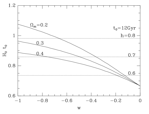
FIG. 1.: The age in Hubble units as a function of $w$ for $\Omega_{M}=0.2$, 0.3 and 0.4. Horizontal lines indicate the value of $H_{0}t_{0}$ required for $t_{0}=12\,$Gyr with $h=0.6$, 0.7 and 0.8. Note that the “age constraint” is strongly $w$ dependent.

We note that there are reasons for only considering $w<0$. The first is the age problem, which is even more severe for $w\geq 0$ (see Fig. 1). The second is that for $w>0$ the energy density in the smooth component decreases faster than $R^{-3}$, implying that the ratio of the energy density in the smooth component to the matter component was even larger at earlier times. This suppresses the growth of density perturbations, and when the spectrum of density perturbations is fixed on large scales by COBE, this leads to too little inhomogeneity on small scales (see Fig. 2) [26]. The case $w=0$ corresponds to the smooth component behaving like pressureless matter; if the smooth component clumped, but only on large enough scales to evade detection ($>50h^{-1}$Mpc), the flatness problem could be solved and the COBE normalization would be the same as sCDM because the growth of density perturbations on large scales would be unaffected. However, the growth of perturbations on small scales would be affected and the problem of producing sufficient small scale structure would be similar to that of hot dark matter. Thus, we dismiss this possibility.

The formation of cosmic structure in a CDM model is dictated by the power spectrum of density perturbations. There are two important changes brought about by the presence of a smooth component: the normalization of the power spectrum based upon the accurate COBE determination of CMB anisotropy on angular scales of around $10^{\circ}$ and the transfer function that describes the growth of density perturbations from the inflationary epoch to the present. For fixed inflationary perturbations, CMB anisotropy on COBE scales is larger (due to the integrated Sachs-Wolfe effect [27]); because of the smooth component there is less growth of density perturbations from the inflationary period until the present.

FIG. 2.: Power-spectrum normalization $10^{5}\delta_{H}$ as determined by the four-year COBE DMR results. The COBE $1\sigma$ error is approximately 10%.

We use the COBE four-year results [28] to normalize the power spectrum (assuming negligible gravity waves and $n=1$) using the method of Ref. [29]. Writing the (linear) power spectrum today as

$$P(k) \equiv \langle|\delta_{k}|^{2}\rangle={2\pi^{2}\over H_{0}^{3}}\delta_{H}^{2}(k/H_{0})^{n}T^{2}(k)$$ (1)

$$T(q) = \frac{\ln\left(1+2.34q\right)}{2.34q}\times$$ (3)

$$\left[1+3.89q+(16.1q)^{2}+(5.46q)^{3}+(6.71q)^{4}\right]^{-1/4}\,,$$

where $\delta_{k}$ is the Fourier transform of the density field, $q=k/h\Gamma$ and $\Gamma\simeq\Omega_{M}h$ is the “shape” parameter [30, 31]. The quantity $\delta_{H}$, which corresponds to the amplitude of density perturbations on the Hubble scale today, is a convenient normalization whose value is shown as a function of $\Omega_{X}$ and $w$ in Fig. 2. The transfer function, $T(k)$, is well fit by the form quoted for $w<0$, with more small-scale power than this form predicts when $w\to 0$.

FIG. 3.: $\sigma_{8}$ as a function of $w$ with $\Gamma=0.25$ and $n=1$. Points with $2\sigma$ error bars on the curves show $\sigma_{8}$ from cluster abundance for that value of $\Omega_{M}$. Note, $\sigma_{8}$ scales as $(\Gamma/0.25)^{1.3}\exp[-3.1(n-1)]$.

There are many constraints on CDM models. The two most stringent for the power spectrum in low-$\Omega_{M}$ models are: the shape parameter $\Gamma=0.25\pm 0.05$ (for $n=1$) [32] and the abundance of rich clusters. The latter can be reduced to a constraint on $\sigma_{8}$ (the rms mass fluctuation in spheres of radius $8h^{-1}$Mpc),

$$\sigma_{r}^{2}\equiv\int_{0}^{\infty}{dk\over k}\ {k^{3}P(k)\over 2\pi^{2}}\,\left({3j_{1}(kr)\over kr}\right)^{2}$$ (4)

with $r=8\,h^{-1}$Mpc. There is no consensus on the precise value of $\sigma_{8}$ or its scaling with $\Omega_{M}$; differences arise due to different input data and calculational schemes [33]. Further, the scaling with $\Omega_{M}$ depends slightly upon $w$, through the relation between virial mass and cluster temperature. Nevertheless, there is a general consensus about this important constraint and as a middle-of-the-road estimate we use $\sigma_{8}=(0.55\pm 0.06)\Omega_{M}^{-0.5}$ which is consistent with most published estimates [33] and slightly conservative (low $\sigma_{8}$) near $\Omega_{M}\sim 0.3$.

There are two nice features of $x$CDM: The shape constraint can be satisfied with $h\sim 0.7$ and $\Omega_{X}\sim 0.6$ for which the $\sigma_{8}$ constraint can be readily satisfied with $w\sim-1/2$ (see Fig. 3). For $\Lambda$CDM ($w=-1$) tilt (i.e. $n<1$) and/or gravity waves are needed to reduce $\sigma_{8}$ and for an open Universe (closely approximated by $w=-{1\over 3}$) $\sigma_{8}$ is too small unless $\Omega_{M}$ is large or $n>1$ [34].

FIG. 4.: Constraints from the SNe-Ia magnitude-redshift diagram. Contours are of $H_{0}r(z=0.4)$ from 0.31 to 0.39 in steps of 0.01. The thick contours are the current 95%CL and 68%CL limits, and arrows indicate that values to the upper right of these curves are favored. (For $w=-1$ the constraint shown here is less stringent than that in Ref. [16] because we have two free parameters rather than one.)

Next, we turn to the two worries of $\Lambda$CDM – the frequency of QSO lensing and the SNe-Ia constraint. Both involve the increased distance to a given redshift that comes with $\Lambda$. The proper distance today is given by the Robertson-Walker radial coordinate [35]

$$r(z) = \int_{0}^{z}{dz\over H(z)}=H_{0}\left[z-{1\over 2}(1+q_{0})z^{2}+\cdots\right],$$ (5)

$$H^{2}(z) = H_{0}^{2}\left[(1+z)^{3}\Omega_{M}+(1+z)^{3(1+w)}\Omega_{X}\right],$$ (6)

and the deceleration parameter $q_{0}=-{\ddot{R}}_{0}/R_{0}H_{0}^{2}={1\over 2}+{3\over 2}w\Omega_{X}$. Note, $r(z)$ increases with decreasing $w$; this leads to more volume and more lenses between us and a QSO at redshift $z$ and a higher frequency of lensing.

While the SNe-Ia limits on the distance redshift relation [16] are quoted for a flat universe with cosmological constant, they are readily translated into a constraint on $r$. Since the seven distant SNe-Ia have redshifts $z\sim 0.4$, that constraint can be expressed as $0.287(0.271)<H_{0}r(z=0.4)<0.342(0.362)$ at 68%CL (95%CL) [36]. Their results constrain $\Omega_{M}$ and $w$ (see Fig. 4). Soon, Perlmutter’s group should have results based on nearly four times as many SNe-Ia’s and another group (The High-z Supernova Team) should have results based on a comparable number of SNe-Ia’s. This will sharpen this important constraint to $w$ significantly.

FIG. 5.: The likelihood, marginalized over $\Omega_{M}$. Contours are in units of ${1\over 2}\sigma$. (See text for the cosmological data and conservative error bars used.)

Concluding remarks. Inflation is a bold and compelling idea. It predicts a flat Universe, but not the form which the critical energy density takes. Because of increasing evidence that the matter density is significantly less than the critical density, as well as the attractiveness of inflation and the successes of CDM, we have explored the possibility that most of the critical energy density resides in a smooth component of unknown nature, with equation of state $p_{X}=w\rho_{X}$ ($w<0$). Increasing $w$ to around $-0.6$ retains the attractive features of $\Lambda$CDM and resolves the conflict with the SNe-Ia constraint; further tilt and/or gravity waves are not required to obtain the correct number of rich clusters observed at present.

For the sake of illustration we have used the following cosmological data to find the best fit $x$CDM model: $t_{0}=15\pm 2\,$Gyr, $h=0.7\pm 0.07$, $\Omega_{\rm B}h^{2}=0.02$, $\Gamma=0.25\pm 0.1$, $\sigma_{8}\Omega_{M}^{0.5}=0.55\pm 0.1$, $[H_{0}r(z=0.4)]^{2}=0.10\pm 0.015$ and the COBE four-year data set. (For several constraints we have inflated the error bars to be conservative.) We have marginalized over $\Omega_{M}$ with prior $\Omega_{M}=0.3\pm 0.05$. For $n=1$, an $x$CDM model with $w=-0.6$ and $h=0.7$ has maximum likelihood (see Fig. 5). (The unmarginalized likelihood prefers $\Omega_{M}\sim 0.4$, $h=0.7$ and $w=-0.4$ but is quite broad.) In passing, we note that a “tangled” network of walls or a wall wrapped around the Universe (supposing space is $S^{2}\times S^{1}$) would lead to a smooth component with $w=-{2\over 3}$.

Introducing $w$ to the list of CDM parameters brings the total to at least ten ($w$, $n$, $h$, $\Omega_{\rm B}h^{2}$, $n_{T}$, $T/S$, $\Omega_{\rm TOT}$, $\Omega_{\nu}$, $\Omega_{X}$, and $\Omega_{\rm RAD}$). While this is a daunting number, the flood of cosmological data coming – larger redshift surveys, accurate measurements of the expansion rate and deceleration rate of the Universe, high resolution observations of clusters with X-rays, the Sunyaev-Zel’dovich effect and weak lensing, studies of galactic evolution by HST and Keck, and especially measurements of CMB anisotropy on angular scales from arcminutes to tens of degrees – should eventually overdetermine the parameters of CDM + inflation. Then the data will not only sharply test inflation, but also discriminate between different CDM models and even provide information about the underlying inflationary potential [37].

In the near term, the SNe-Ia magnitude-redshift diagram and CMB angular power spectrum will provide an important test of $x$CDM: the position of features (e.g., the first peak) in the angular power spectrum tests flatness, but is less sensitive to $w$, and given $\Omega_{\rm TOT}$ (and $\Omega_{M}$), SNe-Ia can determine $w$ (see Fig. 4).

Acknowledgments. This work was supported by the DoE (at Chicago and Fermilab) and by the NASA (at Fermilab by grant NAG 5-2788).

REFERENCES

- [1] See e.g., E.W. Kolb and M.S. Turner, The Early Universe (Addison-Wesley, Redwood City, CA, 1990), Ch. 8.
- [2] M. Bucher A.S. Goldhaber, and N. Turok, Phys. Rev. D 52, 3314 (1995); A.D. Linde and A. Mezhlumian, ibid 52, 6789 (1995); J.R. Gott, Nature 295, 304 (1992).
- [3] See e.g., M. White, D. Scott, and J. Silk, Ann. Rev. Astron. Astrophys. 32, 329 (1994); J.R. Bond, in Cosmology and Large Scale Structure, ed. R. Schaeffer, (Elsevier, Netherlands 1995); W. Hu, N. Sugiyama, and J. Silk, Nature 386, 37 (1997) [astro-ph/9604166].
- [4] S. Dodelson, E. Gates and M.S. Turner, Science 274, 69 (1996).
- [5] See e.g., V. Trimble, Ann. Rev. Astron. Astrophys. 25, 425 (1987); A. Dekel, D. Burstein, and S. White, astro-ph/9611108.
- [6] C. Copi, D.N. Schramm and M.S. Turner, Science 267, 192 (1995).
- [7] M. Strauss and J. Willick, Phys. Repts. 261, 271 (1995); M. Davis, A. Nusser, and J. Willick, Astrophys. J. 473, 22 (1996); J.A. Willick, M.A. Strauss, A. Dekel, and T. Kolatt, preprint (1997).
- [8] See e.g., S.D.M. White et al., Nature 366, 429 (1993); U.G. Briel et al., Astron. Astrophys. 259, L31 (1992); D.A. White and A.C. Fabian, Mon. Not. R. astron. Soc. 273, 72 (1995).
- [9] See e.g., B. Chaboyer, P. Demarque, P.J. Kernan, and L.M. Krauss, Science 271, 957 (1995); M. Bolte and C.J. Hogan, Nature 376, 399 (1995).
- [10] See e.g., W. Freedman, astro-ph/9612024; A. Riess, R.P. Krishner, and W. Press, Astrophys. J. 438, L17 (1995); R. Giovanelli et al, astro-ph/9612072.
- [11] A.R. Liddle et al., Mon. Not. R. astron. Soc. 282, 281 (1996); M. White, P.T.P. Viana, A. Liddle, and D. Scott, ibid 283 107 (1996).
- [12] M.S. Turner, G. Steigman, and L. Krauss, Phys. Rev. Lett. 52, 2090 (1984).
- [13] P.J.E. Peebles, Astrophys. J. 284, 439 (1984);
- [14] L. Krauss and M.S. Turner, Gen. Rel. Grav. 27, 1137 (1995); J.P. Ostriker and P.J. Steinhardt, Nature 377, 600 (1995); J.S. Bagla, T. Padmanabhan and J.V. Narlikar, Comp. Ap. 18, 275 (1996) [astro-ph/9511102]; A.R. Liddle et al., Mon. Not. R. astron. Soc. 282, 281 (1996).
- [15] C.S. Kochanek, Astrophys. J. 466, 638 (1996).
- [16] S.J. Perlmutter et al, astro-ph/9608192.
- [17] S. Weinberg, Rev. Mod. Phys. 61, 1 (1989).
- [18] J. Charlton and M.S. Turner, Astrophys. J. 313, 495 (1987).
- [19] A. Vilenkin, Phys. Rev. Lett. 53, 1016 (1984); D.N. Spergel and U.-L. Pen, astro-ph/9611198.
- [20] R.L. Davis, Phys. Rev. D 35, 3705 (1987); M. Kamionkowski and N. Toumbas, Phys. Rev. Lett. 77, 587 (1996).
- [21] M. Bronstein, Physikalische Zeitschrift Sowjet Union 3, 73 (1933); M. Ozer and M.O. Taha, Nucl. Phys. B287 776 (1987); K. Freese et al., Nucl. Phys. B287 797 (1987); L.F. Bloomfield-Torres and I. Waga, Mon. Not. R. astron. Soc. 279, 712 (1996).
- [22] B. Ratra and P.J.E. Peebles, Phys. Rev. D 37, 3406 (1988).
- [23] K. Coble, S. Dodelson, and J. Frieman, Phys. Rev. D55, 1851 (1996).
- [24] Steinhardt has also suggested parameterizing the equation of state of the smooth component; see, P.J. Steinhardt, in Critical Dialogues in Cosmology, ed. N. Turok (World Scientific, Singapore, 1997).
- [25] In addition to the clumping that is caused by the lumpy matter distribution in the Universe, the X component could also have been slightly perturbed (density variations of order ) to begin with; this would naturally occur if the underlying density perturbations are curvature perturbations (as predicted by inflation). The small amount of clumping of scalar-field energy, tangled strings, or any approximately smooth component, while certainly unimportant for considerations of the distribution of matter today or the evolution of the cosmic-scale factor, will have a small effect on large-angle CMB anisotropy and hence COBE normalization. When the X component is becoming dominant (at relatively recent times), it affects large-angle CMB anisotropy due to the spatially and time-varying gravitational potential it creates (“late-time, integrated Sachs-Wolfe effect”). While the effect of the time-varying potential is included in our work, and is significant, the effect of spatial variations is not. However, in Ref. [22] the effect of spatial variations on the COBE normalization is shown to be small for scalar-field energy.
- [26] The second problem could by circumvented by having the smooth component come into existence recently, e.g., a relativistic sea of particles () can be created by the decay of unstable CDM (see Ref. [12]).
- [27] R.K. Sachs and A.M. Wolfe, Astrophys. J. 147, 73 (1967); L. Kofman and A. Starobinsky, Sov. Astron. Lett. 11, 271 (1985); W. Hu and M. White, Astron. & Astrophys. 315, 33 (1996).
- [28] C.L. Bennett et al., Astrophys. J. 454, L1 (1996).
- [29] E. Bunn and M. White, Astrophys. J. 480, 6 (1997)
- [30] J.M. Bardeen, J.R. Bond, N. Kaiser, and A.S. Szalay, Astrophys. J., 304, 15 (1986).
- [31] N. Sugiyama, Astrophys. J. Supp. 100, 281 (1995); W. Hu and N. Sugiyama, Astrophys. J. 471, 542 (1996).
- [32] J. Peacock and S. Dodds, Mon. Not. R. astron. Soc. 267, 1020 (1994).
- [33] A.E. Evrard, Astrophys. J. 341, L71; J.P. Henry, K.A. Arnaud, Astrophys. J. 372, 410; S.D.M. White, G. Efstathiou, and C.S. Frenk, Mon. Not. R. astron. Soc. 262, 1023 (1993); R. Carlberg et al., J. R. Astron. Soc. Canada 88, 39 (1994); P.T.P. Viana and A. Liddle, Mon. Not. R. astron. Soc. 281, 323 (1996); J.R. Bond and S. Myers, Astrophys. J. Suppl. 103, 63. (1996); V.R. Eke, S. Cole and C.S. Frenk, Mon. Not. R. astron. Soc. 282, 263 (1996) [astro-ph/9601088]; U.-L.Pen, astro-ph/9610147; S. Borgani, A. Gardini, M. Girardi, S. Gottloeber, astro-ph/9702154.
- [34] M. White and J. Silk, Phys. Rev. Lett. 77 4704 (1996); erratum ibid 78, 3799.
- [35] The Taylor series expansion is not very accurate, even for . Padé approximants provide a more accurate approximation; e.g., the second-order Padé approximant is . For all of our results we have numerically integrated the expression for .
- [36] The 95% cl limit to quoted in Ref. [16] is more stringent than that which follows from the 95% cl limit to because the authors of Ref. [16] reduce the number of free parameters from two (, ) to one.
- [37] See e.g., E.J. Copeland, E.W. Kolb, A.R. Liddle, and J.E. Lidsey, Phys. Rev. Lett. 71, 219 (1993); Phys. Rev. D 48, 2529 (1993); M.S. Turner, ibid, 3502 (1993); ibid 48, 5539 (1993).