Projection effects in cluster catalogues

Abstract

We investigate the importance of projection effects in the identification of galaxy clusters in 2D galaxy maps and their effect on the estimation of cluster velocity dispersions. From large N-body simulations of a standard cold dark matter universe, we construct volume-limited galaxy catalogues that have similar low-order clustering properties to those of the observed galaxy distribution. We then select clusters using criteria tailored to match those employed in the construction of real cluster catalogues such as Abell’s. We find that our mock Abell cluster catalogues are heavily contaminated and incomplete. Over one third (34$\pm$6 per cent) of clusters of richness class R$\geq$1 are miclassifications arising from the projection of one or more sub-clumps onto an intrinsically poor cluster. Conversely, 32$\pm$5 per cent of intrinsically rich clusters are missed altogether from the R$\geq$1 catalogues, mostly because of statistical fluctuations in the background count. Selection by X-ray luminosity rather than optical richness reduces, but does not completely eliminate, these problems. Contamination by unvirialised sub-clumps near a cluster leads to an overestimation of the cluster velocity dispersion which can be very substantial even if the analysis is restricted only to galaxies close to the cluster centre. Thus, the distribution of cluster masses – often used to test cosmological models – is a highly unreliable statistic. The median value of the distribution, however, is considerably more robust because the main effect of contamination is to create an artificial tail of high velocity dispersion clusters. Improved estimates of the cluster velocity dispersion distribution require constructing new cluster catalogues in which clusters are defined according to the number of galaxies within a radius about three times smaller than the Abell radius.

1 Introduction

Clusters of galaxies are a major source of cosmological information. Because of their large luminosity they can be detected, and their properties can be measured with relative ease, out to large distances. This makes it possible to exploit their special characteristics as the most massive nonlinear objects in the Universe. In hierarchical clustering theories for the formation of structure, clusters are associated with the rare high peaks in the primordial density field on scales of a few megaparsecs. As a result, their mass and abundance are very sensitive to the amplitude of mass fluctuations on these scales (Frenk et al. 1990; White, Efstathiou & Frenk 1993; Viana & Liddle 1996; Eke, Cole & Frenk 1996b). The epoch of cluster formation and the rate at which the cluster population builds up is, similarly, a strong function of the mean density parameter, $\Omega$ [Lacey & Cole 1993, Eke et al. 1996b], as is their degree of internal substructure (Richstone, Loeb & Turner 1992; Mohr et al. 1995; Wilson, Cole & Frenk 1996). The clustering properties of clusters depend primarily on the shape of the power spectrum of mass fluctuations and have been a subject of much debate for over 20 years [Bahcall & Soneira 1983, Dalton et al. 1994, Eke et al. 1996a]. Finally, rich clusters have recently been used to map the local density field (Plionis et al. 1996, in preparation).

The use of galaxy clusters as cosmological diagnostics relies on the availability of statistical samples, selected according to a well-defined property, such as richness, mass, or X-ray temperature. Traditionally, the source of such samples has been Abell’s (1958) cluster catalogue. The integrity of the Abell catalogue, however, has been questioned over the years (e.g. Fesenko 1979a,b; Lucey 1983; Frenk et al. 1990). Even Abell himself made it quite clear that the completeness and homogeneity of his catalogue were suspect. Partly to overcome these shortcomings new cluster catalogues were constructed in the early 1990s based, as Abell’s, on photographic material, but replacing eye-ball identifications by automated scans of digitized plates. These procedures have produced the APM [Dalton et al. 1992] and Edinburgh-Durham cluster catalogues (EDCC; Lumsden et al. 1992). Computer manipulation of the galaxy images has allowed a degree of uniformity and repeatability to be reached that was impossible in Abell’s days. Nevertheless, Abell clusters remain the best studied, and Abell’s catalogue the main source from which samples are drawn for statistical studies.

Whether by eye or by computer, catalogued clusters are identified as two-dimensional objects, seen against a strongly clustered background. The enormous column depth to a cluster makes projection effects inevitable. Indeed, spectroscopic follow-up of Abell and ACO clusters [Abell et al. 1989] often reveals several clumps of galaxies lined up in the direction to a rich cluster (see Katgert et al. 1996 for a recent study of a large sample). Although these clumps enhance the apparent richness of the cluster, the dominant concentration along the line-of-sight is often rich enough to emit X-rays (e.g. Briel & Henry 1993). This fact alone, however, says little about the importance of projection effects or the completeness of optically selected cluster samples.

Since the abundance of clusters declines very rapidly with richness or mass, even a small amount of contamination can compromise statistical studies in which completeness and/or homogeneity are required. The cluster two-point correlation function is a good example. Values for the correlation length, $r_{0}$, differing by almost a factor of two have been strongly advocated by various workers [Bahcall & Soneira 1983, Postman, Geller & Huchra 1992, Efstathiou et al. 1992, Nichol et al. 1992, Dalton et al. 1994]. According to Bahcall & West (1992) the differences are due to the different limiting richnesses of the various samples but others have claimed that they are due (at least in part) to a misclassification of poor clusters which are placed into a higher Abell richness class as a result of contamination by the halos of rich clusters [Sutherland 1988, Dekel et al. 1989, Efstathiou et al. 1992]. Eke et al. [Eke et al. 1996a] have argued that a combination of different selection procedures and a richness dependence of the clustering strength also contributes to these differences.

While even distant sub-clumps artificially enhance the apparent richness of a cluster, subclustering in its immediate vicinity causes its velocity dispersion to be overestimated (e.g. Frenk et al. 1990). This effect is the likely cause of the poor correlation between the X-ray temperature and velocity dispersion of the most massive clusters [David, Jones & Forman 1995] and it vitiates comparisons between cluster masses determined from X-ray, optical and gravitational lensing data [Fahlman et al. 1994]. The distribution of cluster masses or velocity dispersions has been used as a discriminant of different cosmological models (e.g. Weinberg & Cole 1992; Bahcall & Cen 1993; Lubin et al. 1996). These comparisons tend to rely heavily on the behaviour of the high mass end of the distribution which, unfortunately, is particularly sensitive to contamination due to substructure. Masses derived from X-ray data are more reliable (Evrard, Metzler & Navarro 1996; but see Balland & Blanchard 1995), but since cluster samples are almost invariably selected by their optical properties, the inferred distributions of X-ray properties are also subject to the kind of uncertainties discussed above. Furthermore, by virtue of the fact that optically selected cluster catalogues all have a lower cut-off in richness, there is an in-built bias in these samples against low mass clusters.

It seems clear that the use of cluster properties as cosmological diagnostics requires a detailed understanding of the biases introduced by projection effects and contamination in cluster catalogues. The aim of this paper is to set up a methodology for quantifying such biases using mock galaxy catalogues constructed from N-body simulations. In this paper we analyze mock catalogues constructed from standard $\Omega=1$ cold dark matter (CDM) simulations and we concentrate on Abell clusters. Our procedures, however, can readily be extended to other cosmologies and other cluster catalogues. We also use our mock catalogues for testing alternative procedures for defining clusters and estimating their properties which avoid some of the biases present in Abell’s catalogue. Our work extends previous analyses by Frenk et al. [Frenk et al. 1990] and White (1991,1992) who used similar techniques. An earlier assessment of the completeness and contamination of Abell’s catalogue, using Monte-Carlo simulations, was carried out by Lucey [Lucey 1983]. He found that between 15 and 25 per cent of rich Abell clusters have a true membership that is less than half the number observed. However, his models contained no dynamical information, and they did not take into account the clustering properties of galaxies and clusters.

In Section 2 we give technical details of our simulations and our method for constructing galaxy catalogues from which mock Abell catalogues are derived. The galaxy catalogues encapsulate the essential characteristics of the real situation, although we have not tried to reproduce the observed properties in every detail. Section 3 presents an analysis of the completeness of the cluster catalogues. By identifying groups along the line-of-sight to each cluster, we determine the properties of the main concentration of galaxies, and those of clumps projected onto the cluster. The various categories of contamination we identify are described in Section 4. In Section 5 we discuss how projection effects influence estimates of cluster velocity dispersions derived from radial velocity measurements and illustrate how careful cluster selection and interloper removal can improve upon the accuracy of these estimates. In Sectio 6 we apply a popular statistical test for substructure to our data and demonstrate its potential for flagging clusters whose velocity dispersion estimates are strongly affected by substructure. In Section 7 we present the cluster-cluster correlation function, and illustrate how overlapping clusters can affect the amplitude of this function. Finally, we present a summary of our main results in Section 8.

Figure 1: The real space two-point correlation function of galaxies in our catalogues compared with observations. The solid circles show $\xi(r)$ obtained by averaging over 8 independent simulated galaxy catalogues. The open circles show Baugh’s (1996) deprojection of the angular correlation function of the APM galaxy catalogue. The triangles show the real-space correlation function derived by Loveday et al. (1995) from the Stromlo-APM galaxy redshift survey.

2 Methods

2.1 Simulations

Our analysis employs the set of 8 standard CDM N-body simulations described by Eke et al. [Eke et al. 1996a]. Each simulation followed $128^{3}$ particles in a comoving periodic box 256 $h^{-1}$Mpc on a side, using Couchman’s [Couchman 1991] adaptive P³M code. The mass per particle is therefore $2.2\times 10^{12}{h^{-1}}{{\rm M}_{\odot}}$. The force softening (for an equivalent Plummer potential) was fixed at $\sim 65{h^{-1}}$kpc in comoving coordinates.

Initial conditions were laid down using the CDM transfer function given by Bardeen et al. [Bardeen et al. 1986] (hereafter BBKS) for adiabatic fluctuations in a universe with a negligibly small baryon density and $h=0.5$. Initial velocities and displacements were computed using the Zel’dovich approximation as outlined by Efstathiou et al. [Efstathiou et al. 1985] and Davis et al. [Davis et al. 1985]. The expansion factor $a$ was chosen so that $\sigma_{8}=a$, where $\sigma_{8}$ is the $rms$ amplitude of mass fluctuations in a sphere of radius 8 $h^{-1}$Mpc. Each simulation was started at $a$=0.05 and halted at $a$=0.63, using a time-step $\Delta a$=0.002. Only the final epoch $a$=0.63 was used for the present study. According to White et al. (1993), Viana & Liddle (1996) and Eke et al. (1996b) this normalization is required to obtain approximately the observed abundance of rich clusters.

2.2 Constructing Galaxy Catalogues

It is not yet possible to carry out simulations of cosmological volumes that are large enough to contain many galaxy clusters and have enough resolution to model the dissipative processes of star and galaxy formation. Attempts to introduce galaxies into numerical simulations are therefore subject to considerable uncertainty. We have implemented a scheme that produces galaxy catalogues that match the observed galaxy-galaxy two-point correlation function over the range of separations of interest and on which we can apply a procedure for finding clusters that closely mimics Abell’s selection criteria. The prescription we use is based on the peak-background split technique outlined in BBKS. Further information about the detailed implementation may be found in White et al. [White et al. 1987].

The BBKS formalism gives the number density of peaks of a certain height in a field $F$ filtered on a galaxy scale, $r_{s}$, even though the simulations do not resolve the field, $F$, on that scale, but only on a scale $r_{b}>r_{s}$. The scale $r_{s}$ we associate with individual galaxies and corresponds to ${\sim}10^{12}{{\rm M}_{\odot}}$. Now let $F_{s}$ denote the Gaussian random density field, $F$, smoothed with a Gaussian filter of width $r_{s}$. We associate a galaxy with a density peak in excess of $\nu_{s}\sigma_{s}$, where $\sigma_{s}$ is the $rms$ value of the field $F_{s}$. Similarly, we define the quantities $F_{b}$ and $\sigma_{b}$ for the same field, $F$, now filtered on a scale $r_{b}$. The full expression for the quantity ${\cal N}_{pk}(\nu_{s}|\nu_{b})d\nu_{s}$, the number density of peaks in the field $F_{s}$ with height in the range $\nu_{s}\sigma_{s}$ to ($\nu_{s}+d\nu_{s}$)$\sigma_{s}$, at points where the background field has the value $\nu_{b}\sigma_{b}$, is given in Appendix E of BBKS. In order to ensure that the correlation properties of the galaxies reflect those of the underlying distribution of peaks in $F_{s}$ we choose a suitable filter function to obtain $F_{b}$. By using a sharp low-pass filter in $k$-space, we eliminate the correlations between the difference field $F_{s}-F_{b}$ and $F_{b}$. The price of this is that oscillations in the correlation function of the background field only vanish asymptotically. However, this effect is negligible on the scales of interest and, since we are not seeking to provide an exact match to the galaxy distribution, this scheme is quite sufficient for our purposes.

The procedure outlined above was implemented as follows: the initial density distribution (sampled on a $128^{3}$ grid) was smoothed by removing all power below $r_{b}$=8.75$h^{-1}$Mpc. A tabulated version of ${\cal N}_{pk}(\nu_{s}|\nu_{b})d\nu_{s}$ was then used to find the ’peak number’ associated with each point on the grid of the smoothed initial density field. In order to construct a volume-limited catalogue, we determined the total number of galaxies by requiring that the luminosity density of our model catalogue be consistent with recent determinations of the luminosity function (e.g. Loveday et al. 1992; Marzke et al. 1994). Our adopted value of $\rho_{L}=0.0176L_{*}{h^{3}{\rm Mpc}^{-3}}$ lies in the range bracketed by the observational data which differ by rather large amounts. This normalization reproduces the observed abundance of Abell clusters ($\sim 8\times 10^{-6}{h^{3}{\rm Mpc}^{-3}}$, Scaramella et al. 1991) when we identify clusters using the method described in the next subsection. The only other two parameters $\nu_{s}=1.2$ and $r_{s}=0.54{h^{-1}}{\rm Mpc}$ were chosen to match the observed galaxy-galaxy correlation function, $\xi_{gg}$ (see Figure 1). For our chosen values of $\nu_{s}$ and $r_{b}$, the mean luminosity associated with each peak is 0.87 $L_{*}$, and the mean luminosity associated with each particle is 0.14 $L_{*}$. (With the large number of particles in these simulations, no oversampling is necessary, even in the densest regions; see White et al. 1987). Where necessary, we have assumed that the distribution of galaxy luminosities follows a Schechter function:

$$\phi(L)dL=N_{*}L^{-\alpha}\exp(-L)/\Gamma(2-\alpha)dL,$$ (1)

where $L$ is expressed in units of $L_{*}$, and $\Gamma$ is the gamma function. The final galaxy catalogues are constructed by randomly selecting particles in the simulation volume and identifying them as galaxies with a probability directly proportional to the ‘peak number’ associated with the grid point nearest that particle in the initial conditions. The galaxy inherits from the particle both its position and velocity at later times.

Figure 2: The total luminosity of the main cluster (solid squares), together with the second (crosses) and third (open circles) brightest clumps along the line-of-sight to each cluster, as a function of the galaxy count in 2D. The dashed line represents the 3D luminosity threshold of $43L_{*}$ required for an Abell cluster of richness class R=1. No background count has been subtracted from the 2D cluster richness count.

Figure 3: The X-ray luminosity (within a detect cell of radius 0.75$h^{-1}$Mpc) of the main cluster (solid squares), together with the second (crosses) and third (open circles) brightest clumps along the line-of-sight to each cluster, as a function of the galaxy count in 2D. The dashed line corresponds to a luminosity of 1.8$\times 10^{43}$erg/s, the lowest detection in the survey of Briel & Henry (1993)

2.3 Cluster Selection

Abell defined a rich cluster as an enhancement of galaxies on the Palomar Sky Survey plates. To qualify as a cluster, the number of galaxies within an ‘Abell radius’ ($r_{a}=1.5{h^{-1}}{\rm Mpc}$) from the proposed cluster centre had to exceed a certain number, $n_{a}$, after background subtraction. Galaxies were counted in the magnitude interval between $m_{3}$ and $m_{3}+2$, where $m_{3}$ is the apparent magnitude of the third brightest galaxy. For a cluster of Abell richness class R=1, the lowest richness class that can be considered reasonably complete, $n_{a}\geq 50$, while for a cluster of Abell richness class 2, $n_{a}\geq 80$.

As starting point for the construction of mock catalogues that encapsulate the main features of Abell’s [Abell 1958] cluster catalogue, we use volume-limited galaxy samples. We assume that the luminosity distribution of the cluster galaxies is drawn from a Schechter function as given in equation (1). We construct catalogues that have the correct number of galaxies to cover the interval down to two magnitudes below that of the median value of the third most luminous galaxy drawn from a cluster with a true luminosity equal to that expected for a cluster with R=1. Since the box length in our simulations is smaller than the effective path length to a typical Abell cluster, this limit is equivalent to Abell’s counting limit. The number of galaxies projected onto a typical model cluster, however, is smaller than the number of galaxies along the-line-of sight to a moderately distant Abell cluster. Thus our procedure will underestimate the degree of contamination by distant background galaxies.

Each volume-limited catalogue was projected along the coordinate axes onto three orthogonal planes, thus producing three different 2D galaxy catalogues from each simulation. A friends-of-friends group finding algorithm (Davis et al. 1985) with a linking length 30 per cent of the mean inter-galaxy separation was then applied to the 2D galaxy catalogues. The resulting list of groups is the starting point for the cluster search. (The final cluster catalogues are insensitive to the choice of linking length in the range $\sim 0.3-0.6$.) The total luminosity projected within the Abell radius, $r_{a}$, is $N_{*}L_{*}$. The normalization is thus fixed by the quantity $N_{*}$ which we now calculate.

The cumulative distribution of luminosities is found by integrating the luminosity function

$$\psi(L)\equiv\int_{L}^{\infty}\phi(L^{\prime})dL^{\prime}=\Gamma(1-\alpha,L)N_{*}$$ (2)

where $\Gamma(\alpha,L)$ is the incomplete gamma function. The distribution of the $j$th brightest cluster member is given by

$$\phi_{j}(L)dL=\frac{\psi^{j-1}(L)}{(j-1)!}\exp{[-\psi(L)]}\phi(L)dL,$$ (3)

[Schechter 1976]. For the third brightest galaxy this gives,

$$\phi_{3}(L)dL=\frac{1}{2}\psi^{2}(L)\exp{[-\psi(L)]}\phi(L)dL$$ (4)

and consequently

$$\psi_{3}(L) \equiv \int_{L}^{\infty}\phi_{3}(L^{\prime})dL^{\prime}$$ (5)

$$= 1-\left(1+\psi(L)+\frac{1}{2}\psi^{2}(L)\right)\exp{[-\psi(L)].}$$

The median luminosity of the third brightest galaxy, $\overline{L}_{3}$, is found by solving $\psi_{3}(L)=\frac{1}{2}$, which gives $\psi(\overline{L}_{3})=2.674$ and therefore $\overline{L}_{3}$ is the solution to:

$$\psi(\overline{L}_{3})=\int\limits_{\overline{L}_{3}}^{\infty}\phi(L^{\prime})dL^{\prime},$$ (6)

which yields $\overline{L}_{3}$=2.11. Bearing in mind that Abell’s richness count is defined over a 2 magnitude interval, we get the following relation between the normalization parameter, $N_{*}$, and the galaxy count, $n_{a}$:

$$n_{a}=\frac{N_{*}}{\Gamma(2-\alpha)}\int\limits_{0.1585\overline{L}_{3}}^{\overline{L}_{3}}L^{-\alpha}\exp(-L)dL.$$ (7)

For R=1 clusters, $N_{*}=60$ for $\alpha=1$. $N_{*}$ depends only weakly on the value of $\alpha$ (it varies by less than 10 per cent over the range $\alpha$=1.0$-$1.5). $N_{*}$ is therefore not very sensitive to the highly correlated and poorly constrained luminosity function parameters.

The 50 galaxies between $m_{3}$ and $m_{3}+2$ represent a total luminosity within $r_{a}$ of 60$L_{*}$. Thus, to ensure that all R$\geq$1 clusters in the simulation volume, $V$, are detected requires a volume-limited catalogue with

$$N_{gal}=\rho_{L}\frac{50}{N_{*}L_{*}}V$$ (8)

galaxies. Since the total number of galaxies that resides in the clusters is small compared with the total number in the box, we assume that the contamination by foreground and background galaxies is proportional to the volume projected onto the cluster, i.e. to the number of galaxies within a cylinder of volume $\pi r_{a}^{2}l_{box}$ ($l_{box}=V^{1/3}$) centred on the cluster. Within an Abell radius we expect, on average, 27 background galaxies in addition to at least 50 cluster members.

Each of the groups identified using the friends-of-friends algorithm in the 2D galaxy catalogue was checked to see whether the number of galaxies within the Abell radius exceeded the 76 needed to qualify as an R=1 cluster. The poorer of a pair of overlapping clusters (projected separation $<2r_{a}$) was removed. On average the number of clusters found per catalogue was 139, corresponding to a number density $\sim 8\times 10^{-6}{h^{3}{\rm Mpc}^{-3}}$.

One of the quantities that we wish to calculate is the fraction of clusters that would actually meet Abell’s criterion if this were applied in three dimensions. For this we need to convert the 2D luminosity threshold found above ($N_{*}=60L_{*}$) to a 3D threshold. This requires making a correction for the galaxies that are projected onto the cluster, but lie outside $r_{a}$. We assume that an average spherical cluster can be adequately described by a power-law density profile $\rho(r)\propto r^{-\gamma}$. The correction is the ratio of $M_{p}(r_{a})$, the mass seen in projection within a cylinder of radius $r_{a}$, to the total mass $M(r_{a})$ within the aperture in 3D. For the power-law density profile these masses are,

$$M_{p}(r)=\frac{4\pi}{3-\gamma}r^{3-\gamma}\frac{\Gamma(\frac{1}{2})\Gamma(\frac{\gamma-1}{2})}{2\Gamma(\frac{\gamma}{2})},$$ (9)

$$M(r)=\frac{4\pi}{3-\gamma}r^{3-\gamma}.$$ (10)

Taking $\gamma=2.2$, the value derived by Lilje & Efstathiou [Lilje & Efstathiou 1988] from their determination of the cluster-galaxy cross-correlation function, we find a ratio $M(r_{a})/M_{p}(r_{a})$=0.72 and therefore a 3D threshold for richness class R$\geq$1 of $43L_{*}$. The assumed value of $\gamma$ is in good agreement with $\gamma=-2.3\pm 0.4$ found directly from the luminosity weighted particle distribution over the interval between 0.1 and 1.5 $h^{-1}$Mpc. The mean slope found for the 2D cluster catalogue is $-2.0\pm 0.3$, slightly lower as a result of contamination caused by projection effects.

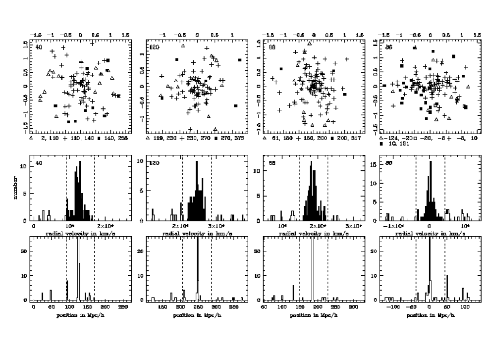
Figure 4: The top panel shows the distribution of galaxies in two R=1 clusters (numbers 40 and 120, left two columns) and two R=2 clusters (numbers 68 and 86). Different sections along the line-of-sight have been plotted with different symbols, as indicated in the legend at the bottom of each figure. (The numbers in the legend are intervals in units of Mpc/h.) Open symbols are used for galaxies in front and solid symbols for galaxies behind the cluster, while crosses denote galaxies that belong to the cluster. The middle row shows the corresponding distribution of radial velocities in a cylinder centred on the cluster. The shaded part of the histogram shows the galaxies that are classed as cluster members after a $3\sigma$ clipping procedure (see below); the unshaded regions have been classed as foreground and background objects. The lower panel shows true positions along the line-of-sight. Note that these lower two panels are centred on the cluster. The dashed lines denote an 8000 km/s window, centred on the cluster, used to make an initial selection for the determination of velocity dispersions. These clusters are only weakly contaminated by projection effects.

3 The Completeness of Cluster Catalogues

The effects of contamination by foreground and background galaxies on the completeness of the Abell catalogue were first considered by Lucey [Lucey 1983]. His Monte-Carlo simulations, however, were crude because they did not take into account the clustering of the contaminating galaxies. By contrast, our mock galaxy catalogues reproduce the low-order clustering statistics of the real galaxy distribution over the range of scales of interest and so they provide a much better approximation to the source of projection effects.

To investigate the reality of clusters identified in projection, we compare our mock 2D cluster catalogues with catalogues of clusters identified in 3D. The latter were constructed from the centres returned by the friends-of-friends group finder applied to the dark matter distribution, using a linking length of 10 per cent of the mean inter-particle separation. (Again, the results are insensitive to this choice.) The luminosity of these 3D clumps was calculated by summing over the total luminosity associated with the particles contained within a sphere with radius 1.5$h^{-1}$Mpc. Only groups with more than eight particles were considered. With each 2D ‘Abell’ cluster, we associate all 3D clusters whose centres fall within the Abell radius of the projected cluster. Figure 2 shows the distribution of luminosities of the three most luminous 3D groups identified along the line-of-sight towards each Abell richness class R$\geq$1 cluster in one of our 24 catalogues. The 3D threshold of 43$L_{*}$ required for richness class R=1 is shown by the dashed line. Averaged over all galaxy catalogues, we find that 34 $\pm$6 per cent of ‘Abell’ clusters are not associated with a 3D cluster which, on its own, meets the generalized Abell criterion. These clusters are only seen above the threshold in projection because of the superposition of several sub-threshold clumps along the line-of-sight. Conversely, we find that 32$\pm$5 per cent of the 3D clumps brighter than 43$L_{*}$ fail to be picked out as Abell clusters in projection. In most cases, such non-detections are due to fluctuations in the background count as a result of which intrinsically rich clusters are misclassified as poorer groups. In addition, in 5 per cent of cases, we find that two 3D clumps above the threshold are associated with a single 2D object. Thus, in our simulations, about a third of clusters classified as Abell R$\geq$1 clusters are, in fact, poorer groups, whilst a similar fraction of intrinsically rich clusters, are not included in the catalogue at all. We conclude that catalogues selected using Abell’s criteria are neither homogeneous nor complete to a uniform integrated luminosity limit.

X-ray emission from the hot intra-cluster medium provides an alternative means of selecting cluster samples. No extensive sample selected exclusively on the basis of X-ray data exists to date. A first step in this direction is the catalogue of clusters compiled by Romer et al. (1994) who correlated a sample of X-ray sources with optical galaxy counts from digitized photographic plates. In most studies however, the cluster catalogue is taken as the starting point for further selection according to X-ray flux or luminosity (e.g. Nichol, Briel & Henry 1994). Any incompleteness present in the cluster catalogue is then automatically carried forward to the X-ray sample. Nevertheless, it is of interest to ask how such X-ray cluster samples are further affected by projection effects. Our simulations do not follow the gas component responsible for the X-ray emission from clusters. However, we can use the results of recent N-body/gasdynamics simulations of the formation of individual clusters to calculate, approximately, the expected X-ray luminosity from our clusters. These simulations show that the collapse and shock heating of a non-radiative gas during cluster formation establishes a near equilibrium configuration in which the density profile of the gas closely follows that of the dark matter (Evrard 1990; Thomas & Couchman 1992; Navarro, Frenk & White 1995, but see Anninos & Norman 1996). We can therefore estimate the expected X-ray emission from a cluster by associating with each particle in our simulations an ‘X-ray luminosity’ proportional to the product of the local density and velocity dispersion, $L_{x}\propto\rho\sigma_{v}$. Both these quantities are calculated by averaging over the 10 nearest neighbours of each particle. When summed over a group of particles, the total ‘X-ray luminosity’ has the same dependence on temperature and density as Bremsstrahlung emission, $L_{x}\propto\rho^{2}T_{x}^{0.5}$.

Figure 3 shows the ‘X-ray luminosities’ of the same clusters plotted in Figure 2. The model luminosities were normalized by setting the median luminosity of the brightest sub-clump along each line-of-sight equal to $10^{44}$erg/s, close to the median X-ray luminosity in the 0.5-2.5 keV band of a sample of 145 high galactic latitude Abell clusters studied by Briel & Henry [Briel & Henry 1993]. These luminosities were calculated in an inner sphere of radius 0.75$h^{-1}$Mpc, similar, in projection, to the optimal detect area recommended by Briel & Henry for their sample. The dashed line in the Figure corresponds to a luminosity of 1.8$\times 10^{43}$erg/s, the lowest 0.5-2.5 keV rest-frame X-ray luminosity detected by Briel & Henry. These authors detected only 46 per cent of the 145 clusters in their sample. In part this is due to uneven sky coverage which also leads to upper limits on non-detections that vary between 1.6$\times 10^{43}$ and 2.7$\times 10^{44}$erg/s. These variable limits preclude any conclusions regarding the completeness of the X-ray samples. Nevertheless, Figure 3 shows that even X-ray selection is not immune from projection effects. A significant fraction (16 per cent) of the second-ranked clumps and even some of the third-ranked clumps along the line-of-sight have X-ray luminosities above the minimum detected in the data. In a few cases, the second-ranked clumps have comparable luminosities to the first-ranked clumps. Only the brightest clusters, those with $L_{X}\lower 3.22916pt\hbox{$\sim$}\hbox to0.0pt{\hss\raise 1.1625pt\hbox{$>$}}10^{44}$ erg/s, provide a clean, although not necessarily complete, sample. We therefore conclude that even X-ray selected samples are, to some extent, contaminated by projection effects, although this seems to be a weaker effect than for optically-selected samples. Projection effects are reduced because of the high central concentration of the X-ray emission and the use of a relatively small detect area. Examination of an analogous plot to that in Figure 3, using X-ray luminosities within 1.5$h^{-1}$Mpc rather than within 0.75 $h^{-1}$Mpc, shows that projection effects are much stronger for the larger detect areas.

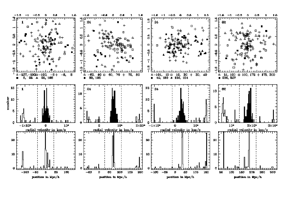
Figure 5: As Figure 4, but for mildly contaminated clusters. The main galaxy concentration in these clusters still has richness R$\geq$1 after contamination has been removed. Such clusters clearly belong in the Abell catalogue, but their richness has been artificially enhanced by projection effects.

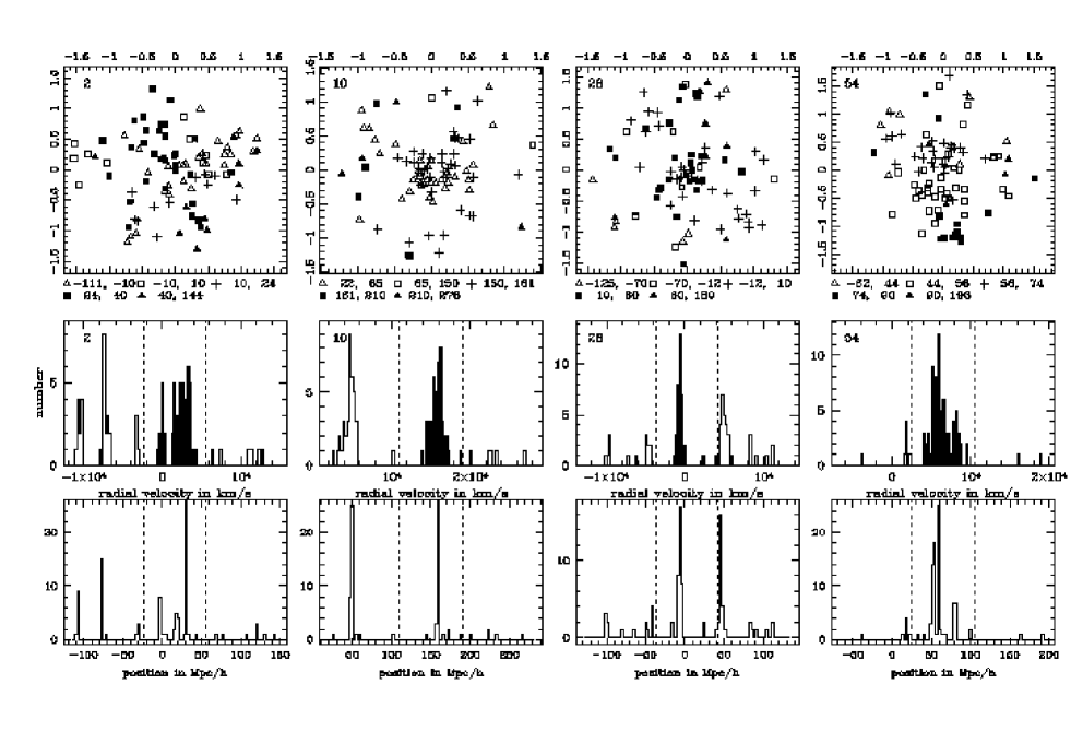
Figure 6: As Figure 4, but for severely contaminated clusters. The main galaxy concentration in these clusters has R$<$1 after projection effects are removed. These clusters should not have been included in the Abell catalogue.

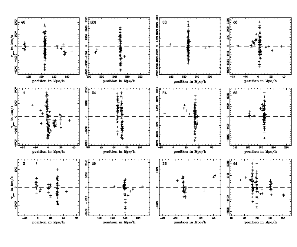
Figure 7: The radial component of the peculiar velocity plotted against the line-of-sight position of galaxies in clusters. The top row shows the R=1 and R=2 clusters of Figure 4, the middle row shows the mildly contaminated clusters of Figure 5, and the bottom row shows the severely contaminated clusters of Figure 6.

4 Structure in the redshift space direction

The ‘optically selected’ clusters found using the techniques outlined above show considerable variation in structure and richness. A significant fraction, $\sim$ 30-40 per cent, of the R$\geq$1 clusters are almost uncontaminated and clearly meet the criterion derived above for an Abell cluster in 3D. Examples of such clusters are shown in Figure 4. The lower panel shows a histogram of the true spatial distribution of galaxies along the line-of-sight, in bins of width 2.56$h^{-1}$Mpc (The vertical axis has been cut off at 26 galaxies.) These distributions are dominated by a single concentration which is much richer than any of the sub-clumps along the line-of-sight. The middle row shows the distribution of radial velocities of all galaxies in the direction to the cluster. The histograms are not always Gaussian or even symmetric (Note the high velocity tail at $cz$=20,000km s^-1 in cluster 68), even though the cluster galaxies are well localized in space. (All cluster members in the lower panel of cluster 68 fall in a single 2.56$h^{-1}$Mpc bin.) The top row shows the distribution of galaxies on the sky. Different symbols indicate background, foreground and cluster members (on the basis of the positional information in the lower row). All clusters appear regular and, in many cases, quite spherical. Although this is typical of practically all uncontaminated clusters, there are a few examples of elongated objects (e.g. cluster 86).

The remaining 60-70 per cent of clusters suffer from some kind of projection effect. Figure 5 shows four examples of clusters that have been contaminated by other structures. In these cases, had contamination been removed, the richest remaining group along each line-of-sight would still have qualified as an R=1 cluster. Although the velocity histograms do not differ greatly from those of the uncontaminated clusters in Figure 4, closer inspection reveals that, in some instances, the foreground and background groups appear to form identifiable structure when viewed face-on (e.g. the open triangles in cluster 62); in other cases the contaminating galaxies are distributed randomly over the entire field (e.g. solid squares in cluster 1). Cluster 24 is an example of a binary cluster. The smaller component, containing about 30 galaxies (open squares), is located 5 $h^{-1}$Mpc in front of the main cluster which contains $\sim$55 galaxies. Yet, the radial velocity distribution in the middle panel is quite symmetric and shows no clear evidence of bimodality. Although these projection effects are not as severe as those that lead to poor groups being detected and classed as rich clusters, they affect the richness assigned to a cluster and compromise statistical studies including, for example, estimates of the cluster abundance as a function of richness.

More extreme cases of misidentification and misclassification are shown in Figure 6. The main peak on which the histograms are centred was found by filtering with a 4000 km s^-1 top hat function. The main galaxy concentration fails to meet the 43$L_{*}$ luminosity criterion for an R=1 Abell cluster in 3D, although the clusters do meet the 2D criterion of more than 50+27 galaxies in projection. A significant fraction of all clusters that fall into this category are not as centrally concentrated as the clusters in Figures 4 and 5. However a surprisingly large number looks little different, considering that they are pure superpositions. We find a great variety in the nature of these superpositions. Some consist of multiple groups of roughly comparable richness (e.g. clusters 2 and 54), others of two main clumps of comparable size (e.g. cluster 10).

Closer inspection of the histograms of a random subset of all our R$\geq 1$ clusters reveals that in roughly 14 per cent of cases the main peak along each line of sight fails to contain even the 30 galaxies required for an R=0 classification. In 36 per cent of clusters the count lies between 30 and 50 (R=0), in 40 per cent between 50 and 80 (R=1) and in 10 per cent above 80 (R$\geq$2). An average R=1 cluster contains 66 per cent of the galaxies that, when projected, form the cluster in 2D. This is in excellent agreement with our background estimate.

Although it is often assumed that the radial velocities of virialized clusters follow a Gaussian distribution, even a small subcluster can cause a detectable asymmetry. We have examined the degree to which the radial velocity distribution is Gaussian using a variety of indicators. In addition to calculating the skewness and kurtosis of the radial velocity distribution, we have also applied a Lilliefors test (a Kolmogorov-Smirnov test that takes into account the fact that both the mean and dispersion are estimated from the dataset itself). In all cases we estimate confidence intervals by comparing the distribution of normalized ‘observed’ velocities, $z_{i}=(v_{i}-\overline{v})/\sigma$, with random samples drawn from a normal distribution. All three tests find that, at the 95 per cent confidence level, between 45 and 55 per cent of clusters identified in 2D have velocity distributions which are inconsistent with being Gaussian. The percentage of clusters rejected at 90 per cent and 99 per cent confidence levels are $\sim 55$ per cent and $\sim 35$ per cent respectively.

Another illustration of the effects of sub-clumping is given in Figure 7. Here we plot the peculiar velocities, $v_{pec}=v_{r}-v_{H}$, where $v_{H}$ is the Hubble velocity, against position ($v_{H}/H$) for galaxies in the twelve clusters shown in Figures 4-6. (In each case we have limited the total range along the line-of-sight to 100$h^{-1}$Mpc for clarity on smaller scales.) Even those clusters which we earlier regarded as essentially ‘clean’ (top row) suffer from small amounts of contamination. The fraction of clusters that does not have a group of at least 5 members projected onto its face is below 2 per cent. In a number of cases the mean of the peculiar velocity distribution is noticeably displaced from zero, as a result of motions induced by distant matter or by the proximity of a massive neighbouring cluster. This is clearly seen in the case of the ‘binary’ cluster (number 24) and in the case of the multiple cluster (number 54). Several examples show infalling sub-clumps. Just in front of the main mass concentration in cluster 86, a group of 15 galaxies is falling into the cluster, with velocities that increase towards the cluster core. A similar situation occurs in cluster 1, but now there are at least two sub-clumps falling in from different directions. In cases where the cluster fails to meet the criterion for inclusion in the 3D ‘Abell catalogue’, the number of different small subclusters or groups that make up the 2D cluster can be substantial (e.g. cluster 54).

Figure 8: Comparison of ‘true’ velocity dispersions ($\sigma_{v,3D}$) and various ‘observational’ estimates ($\sigma_{v,2D}$). In all cases, the ‘true’ values are $1/\sqrt{3}$ times the 3D velocity dispersion of the dark matter particles within a sphere of the appropriate radius. (a) Clusters identified using Abell’s criterion and $\sigma_{v,2D}$ estimated using an optimistic 3$\sigma$ clipping procedure applied to all galaxies projected within the Abell radius. (b) Clusters identified using Abell’s criterion and $\sigma_{v,2D}$ estimated using an optimistic 3$\sigma$ clipping procedure applied only to galaxies projected within a circle of 0.5$h^{-1}$Mpc radius. (c) Clusters identified using a scaled version of Abell’s criterion to a radius of 0.5$h^{-1}$Mpc and $\sigma_{v,2D}$ estimated using an optimistic 3$\sigma$ clipping procedure on the galaxies projected within this radius. (d) Clusters identified using Abell’s criterion and $\sigma_{v,2D}$ estimated using the interloper removal algorithm of den Hartog & Katgert (1996).

5 Cluster velocity dispersions

The velocity dispersions of galaxy clusters, or the cluster masses derived from them, are an important cosmological diagnostic. They have been used, for example, to test specific cosmological models (Weinberg & Cole 1992; Bahcall & Cen 1993; Lubin et al. 1996), and to estimate the amplitude of mass fluctuations on cluster scales [Evrard & Henry 1991, White et al. 1993, Eke et al. 1996b]. The distribution of velocity dispersion is often used in cumulative form, $n(>\sigma_{v,los})$, the number density of clusters with line-of-sight velocity dispersion greater than $\sigma_{v,los}$. A closely related quantity is the cumulative X-ray temperature function, $n(>T_{X})$, derived from X-ray observations in the central parts of clusters.

Frenk et al. [Frenk et al. 1990] calculated $n(>\sigma_{v,los})$ for an ensemble of $\Omega=1$ CDM simulations and Weinberg & Cole [Weinberg & Cole 1992] calculated this quantity for various Gaussian and non-Gaussian models with $\Omega$=1 and $\Omega$=0.2. On the observational side, Mazure et al.  [Mazure et al. 1996] have recently estimated $n(>\sigma_{v,los})$ for a sample of 80 clusters from the ACO catalogue [Abell et al. 1989]. They determined each $\sigma_{v,los}$ using at least 10 (and in 48 out of 80 clusters more than 30) radial velocities per cluster. These data represent a considerable improvement upon previous compilations (e.g. Zabludoff et al. 1993; Bahcall & Cen 1993).

The main concern when estimating cluster velocity dispersions is the effect of contamination by unvirialized sub-clumps whose coherent motion remains hidden by the amplitude of the peculiar velocities in the cluster region. As Figures 4-6 show, it is not uncommon for a superposition of clumps, separated by 10 Mpc or more, to produce an apparently symmetric and featureless radial velocity distribution. Using our mock catalogues, we now examine the accuracy of various conventional methods for estimating velocity dispersions in ‘observational’ (from now on referred to as 2D) cluster samples by comparing results obtained from them with the ‘true’ velocity dispersions computed directly using the full phase-space information for the dark matter particles within a spherical aperture.

To estimate the velocity dispersion of our 2D samples, we first convolved the ‘observed’ velocity histogram with a 4000 km s^-1 top hat filter in order to reject obvious interlopers and obtain an initial estimate of the mean radial velocity of the cluster. All galaxies with relative velocities greater than 4000 km s^-1 from the peak of the convolved histogram were then excluded from the sample. Next, we applied a standard optimistic $3\sigma$-clipping procedure [Yahil & Vidal 1977] which consists of the following steps: (i) estimate the mean radial velocity $\overline{v}$ and velocity dispersion $\sigma$; (ii) delete all galaxies with radial velocity greater than $3\sigma$ away from $\overline{v}$; (iii) estimate $\overline{v}$ and $\sigma$ for the culled sample; and (iv) remove the most extreme galaxy if its radial velocity is greater than $3\sigma$ from $\overline{v}$. Steps (iii) and (iv) are repeated until the number of galaxies stabilizes. This procedure returns a robust and stable estimate of the cluster velocity dispersion, $\sigma_{v,2D}$.

In panel (a) of Figure 8 we plot the values of $\sigma_{v,2D}$ obtained by applying this method to the clusters in one of our mock Abell catalogues against the true values, $\sigma_{v,3D}$, obtained using all the dark matter particles within the Abell radius, $r_{a}$, of each cluster. (The latter are $1/\sqrt{3}$ times the full 3D velocity dispersion of the dark matter particles.) All qualifying galaxies projected within $r_{a}$ were used in the estimate of $\sigma_{v,2D}$. There is a very poor correlation between these estimates and the true dispersions. In particular, the 2D distribution has a tail of high dispersion clusters which is completely spurious. The true distribution contains only 1 cluster with $\sigma_{v,3D}>1250$ km s^-1 and none with $\sigma_{v,3D}>1500$ km s^-1. Yet the ‘observational’ sample has 33/153 clusters with $\sigma_{v,2D}>1250$ km s^-1and 20/153 with $\sigma_{v,2D}>1500$ km s^-1. These artificially large dispersions are caused by unvirialized clumps of galaxies projected onto the main cluster. A good example is cluster 40, shown in Figures 4 and 7. The derived dispersion for this cluster is $\sigma_{v,2D}=1400$ km s^-1, much larger than the true value $\sigma_{v,3D}=1020$ km s^-1. The main culprit is a group of 8 galaxies located 35 $h^{-1}$Mpc in front of the cluster which is not eliminated by the optimistic 3$\sigma$ clipping procedure. According to a Lilliefors test, the hypothesis that the radial velocity distribution of this cluster is Gaussian cannot be rejected with more than 25 per cent confidence.

In practice, velocity dispersions for real clusters are most commonly estimated using only central galaxies, rather than galaxies spread out over the entire Abell circle, as we have assumed in panel (a) of Figure 8. In panel (b) of this figure we show the result of estimating $\sigma_{v,2D}$ from galaxies projected only onto the inner 0.5 $h^{-1}$Mpc of the cluster. By sampling a smaller area, the number of contaminating clumps is reduced and, as a result, the spurious tail of high $\sigma_{v,2D}$ clusters is diminished but not altogether eliminated. The correlation between $\sigma_{v,2D}$ and $\sigma_{v,3D}$ remains rather poor. As before, dispersions for a substantial fraction of the population are overestimated and, in several cases, they are significantly underestimated.

The main reason why restricting the radial velocity sample to the inner regions of the cluster does not produce a more satisfactory result is that the criteria used to select clusters in the first place already produces a heavily contaminated catalogue. This is due to the large search radius employed by Abell. To illustrate this point we construct a new set of cluster catalogues in which the search radius has been reduced by a factor of three, to 0.5 $h^{-1}$Mpc. Assuming a mean radial density profile, $\rho(r)\propto r^{-2.2}$, the number of galaxies required for richness class R$\geq$1 within this reduced radius is 24. This scaled Abell criterion produces different cluster catalogues than Abell’s standard criterion. We now apply the same optimistic $3\sigma$ clipping procedure as before (using galaxies within 0.5 $h^{-1}$Mpc). The resulting values of $\sigma_{v,2D}$ are compared with the true values, $\sigma_{v,3D}$ (now calculated using dark matter particles within a sphere of radius 0.5 $h^{-1}$Mpc) in panel (c) of Figure 8. The result is considerably better. Virtually all the spurious large dispersions are eliminated and the correlation between the 2D estimates and the true values is considerably tighter.

The dramatic improvement shown in panel (c) cannot, of course, be achieved in practice without replacing Abell’s catalogue by a different one constructed using a smaller search radius. The APM cluster catalogue [Dalton et al. 1992] fulfills this criterion although the search radius of 0.75 $h^{-1}$Mpc  is somewhat larger than our recommended value of 0.5 $h^{-1}$Mpc because the latter did not yield a sufficient number of galaxies in the APM data. However, a weighting scheme was applied which reduces the weight of galaxies in the outer 0.25 $h^{-1}$Mpc ring. Our mock catalogues indicate that the velocity dispersion distribution of APM clusters should be considerably more reliable than that of Abell clusters. Unfortunately an extensive redshift survey of APM clusters has yet to be undertaken.

Finally, we have tested the interloper removal method proposed by den Hartog & Katgert [den Hartog & Katgert 1996]. This method attempts to find an acceptable range for the radial velocities to be included in the galaxy sample depending upon the projected distance from the cluster centre. Using an iterative scheme, the method rejects galaxies with radial velocities differing by more than $v_{max}(R)$ from the systemic velocity, where $v_{max}(R)$ is the maximum of the line-of-sight component of two velocities: (a) the infall velocity for all positions along the line-of-sight at a given projected separation, R, from the cluster centre, and (b) the circular velocity. In order to calculate the infall velocity a value of $\Omega$ must be assumed, but den Hartog & Katgert [den Hartog & Katgert 1996] found that their results do not depend significantly on the choice of $\Omega$. This method succeeds in eliminating more galaxies than the optimistic 3$\sigma$ clipping routine. The comparison between the velocity dispersions obtained using this method and $\sigma_{v,3D}$ is shown in panel (d) of Figure 8. The ‘observational’ estimates correlate better with the true values than the estimates used in Figures 8(a) and 8(b), but not as well as those in Figure 8(c). The den Hartog-Katgert method tends to underestimate most velocity dispersions by $\sim 100$ km s^-1while, at the same time, failing to completely remove the spurious tail of large dispersions.

Figure 9: The cumulative distribution of cluster velocity dispersions based on all our synthetic cluster catalogues. The solid squares show velocity dispersions derived from all galaxies projected within $r_{a}$ from the cluster centre and the open squares from galaxies within $r_{a}/3$ (both using $3\sigma$ clipping to remove interlopers). The triangles were computed from our catalogues using the den Hartog & Katgert interloper removal algorithm. The same algorithm was applied by Mazure et al. (1996) to a sample of 80 ACO clusters and is shown here as the solid circles. The open circles were derived from Bahcall & Cen’s (1993) mass function. The dashed line shows $n(>\sigma_{v,2D})$ for clusters selected in 2D using an Abell criterion scaled to $r_{a}/3$. The “true” distribution, calculated from the velocity dispersion of the dark matter within $1.5{h^{-1}}{\rm Mpc}$ is shown by the solid line.

The cumulative distributions of velocity dispersion returned by the various methods discussed above are compared with the true distribution in Figure 9. The former were constructed by combining data from all 24 mock cluster catalogues. The true distribution, calculated from the velocity dispersion of the dark matter particles within 1.5$h^{-1}$Mpc of the centre, is shown as the solid line. (All clusters with $\sigma_{v,los}>500$ km s^-1 are included.) These data agree well with the cumulative mass distribution of clusters calculated by White et al. (1993) from N-body simulations of the same model. The different symbols show the distributions derived for the mock Abell cluster samples using different methods: the solid squares are the estimates obtained by applying the optimistic $3\sigma$ clipping to all galaxies within $r_{a}$; the open squares correspond to the case when this estimator is applied only to galaxies within $r_{a}/3$; the solid triangles give the result of using the den Hartog-Katgert method. The dashed line shows the distribution of dispersions for clusters identified in 2D but using a reduced search radius of $r_{a}/3$ and the scaled Abell richness criterion. The dispersions in this case were also derived using the 3$\sigma$ clipping procedure. (Note that the total number of clusters identified in this case is about a factor of 2 larger than the number of Abell clusters.)

At values of the velocity dispersion below $\sim 850$ km s^-1 all the distributions from the mock catalogues in Figure 9 include only a steadily decreasing fraction of all the clusters present in the simulation. This turnover simply reflects the threshold richness required for selection which biases the sample against low-$\sigma_{v}$ clusters. At large values of the velocity dispersion, only the distribution for clusters identified with a small search radius approximates the true distribution. All other catalogues overestimate the number of high dispersion clusters by large factors. Even the den Hartog-Katgert method which slightly underestimates the dispersion of small clusters over-predicts the abundance of clusters with $\sigma_{v,los}>1500$ km s^-1 by a factor of $\sim 5$. Note, however, that the tail of the distribution is exaggerated in a logarithmic plot like this. In fact, at the typical abundance of Abell R$\geq$1 clusters, all methods perform quite well. For example, the velocity dispersion at an abundance of $4\times 10^{-6}$ $h^{3}{\rm Mpc}^{-3}$, half the abundance of R$\geq$1 clusters, the dispersions obtained from the different methods lie within $\sim 150$ km s^-1 of the true value. Thus, while the median velocity dispersion of the Abell cluster population is reasonably well determined, the high dispersion tail of the distribution is extremely uncertain. Figure 9 indicates that statistical studies based on the median mass or velocity dispersion of the Abell cluster population (e.g. White et al. 1993) are robust whereas studies that concentrate on the tail of the distribution (e.g. Bahcall & Cen 1993) are unreliable. The APM and EDCC catalogues have a higher number density and are less affected by projection effects than R$\geq$1 Abell clusters. One would therefore expect a sample of such clusters to show a reduction in the spurious high-$\sigma_{v}$ tail compared with a sample of Abell clusters

Also plotted in Figure 9 are two determinations of $n(>\sigma_{v,los})$ from observational samples. The solid circles show the estimate by Mazure et al.  [Mazure et al. 1996] for a sample of 80 clusters analyzed with the den Hartog-Katgert algorithm. The open circles show an estimate derived from Bahcall & Cen’s (1993) mass function of clusters, assuming that the transformation between mass and velocity dispersion is that given by their equation (3) for an isotropic distribution of galaxy velocities. The two observational estimates lie below the model predictions. This is consistent with the results of Frenk et al. (1990), White et al. (1993) and Eke et al. (1996b) which show that the abundance of clusters is correctly reproduced in a CDM model only if $b\simeq 2$.

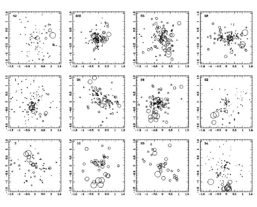
Figure 10: The Dressler-Schectman test applied to mock clusters. The symbols show the projected positions of galaxies in our mock catalogue. The radius of each circle is proportional to $\exp{\delta_{i}}$, where $\delta_{i}$ is a measure of the local deviation of the radial velocity and velocity dispersion from the average values for the cluster as a whole. Foreground and background galaxies have been removed prior to applying the test using a $3\sigma$-clipping procedure.

Figure 11: The correlation between velocity dispersion estimates and the strength of the substructure signal as measured by Dressler & Schectman’s $\Delta$ parameter. In the left panel, foreground and background galaxies were removed using an iterative $3\sigma$ clipping procedure. On the right, the den Hartog-Katgert algorithm (see text for details) was applied to galaxies with a projected separation of less than 1$h^{-1}$Mpc from the cluster centre.

6 Substructure

Substructure in a cluster is symptomatic of a recent merger or accretion event. Typical survival times of accreted groups and subclusters are comparable to the crossing time (a few times $10^{9}$ yr) and thus shorter than the age of the main cluster (Evrard 1990, Gonzalez-Casado, Mamon & Salvador-Sole 1994). The presence of substructure is therefore related to the recent history of a cluster and provides a useful way of constraining cosmological models in which cluster growth rates differ (Richstone et al. 1992; van Haarlem & van de Weygaert 1993; Bartelmann et al. 1993; Mohr et al. 1995; Wilson et al. 1996). In practice, however, identifying substructure in a cluster using the properties of its galaxy distribution is difficult, and the results depend upon the test used to define and detect substructure.

Many statistical tests have been proposed over the years to measure substructure. The first attempts employed only 2D-data. For example, Geller & Beers [Geller & Beers 1982] made contour plots based on Dressler’s [Dressler 1980] measurements of galaxy positions on the sky and concluded that $\sim 40$ per cent of clusters showed signs of substructure. This claim was contradicted by West & Bothun [West & Bothun 1990] and by Rhee, van Haarlem & Katgert [Rhee et al. 1991] who applied a range of statistical tests but found little evidence for substructure in the projected galaxy distribution in the inner regions of clusters. The inclusion of radial velocity data allowed more powerful tests to be developed using all observable properties of the cluster phase-space distribution. Dressler & Shectman [Dressler & Shectman 1988] applied the test that will be described below to a sample of 15 clusters with an average of 73 measured redshifts per cluster. They found evidence for substructure in $\sim 40$ per cent of cases. Bird [Bird 1994] has claimed that as many as 85 per cent of well-studied clusters show some evidence for substructure. To some extent these disparate results are due to different definitions of substructure. Nevertheless, the fact that substructure has been detected even in the Coma cluster (Fitchett & Webster 1988; Mellier et al. 1988; White, Briel & Henry 1993, Colless & Dunn 1995, Biviano et al. 1996), usually regarded as the archetypal relaxed rich cluster, indicates that inhomogeneities are more prevalent than at first thought.

We can use our mock cluster catalogues to assess some of the most widely used methods for characterising substructure and to test ways in which these methods may be used to improve cluster mass determinations from optical data. It should be noted that our detailed quantitative results will depend on our assumed cosmological model, particularly on our adopted value of $\Omega=1$. This choice leads to more prevalent substructure than models with a low value of $\Omega$ (Richstone et al. 1992, Mohr et al. 1995, Wilson et al. 1996). Specifically, we consider here the algorithm proposed by Dressler & Shectman (1988) which attempts to identify dynamically distinct subunits within the cluster. This test is sensitive to local deviations of the mean velocity and velocity dispersion relative to the global values determined for the cluster as a whole. For each galaxy in the sample, a local mean velocity $\overline{v}_{local}$ and a local velocity dispersion $\sigma_{local}$ are computed using the radial velocities of the galaxy itself and of its 10 nearest projected neighbours. The combined deviations are given by the quantity

$$\delta_{i}^{2}=\frac{11}{\sigma^{2}}\left[\left(\overline{v}_{local}-\overline{v}\right)^{2}+\left(\sigma_{local}-\sigma\right)^{2}\right].$$ (11)

The test statistic, $\Delta$, is the mean value of $\delta_{i}$ averaged over all galaxies in the sample.

We computed $\Delta$ for our mock clusters using the same galaxies that were considered when calculating velocity dispersions in Section 5 (i.e. after $3\sigma$-clipping or the application of the den Hartog & Katgert algorithm). The results are illustrated in Figure 10 as a series of plots for the 12 clusters used as examples throughout this paper. Each galaxy is represented by a circle with radius proportional to $\exp({\delta_{i}})$. Individual galaxies with discordant radial velocities occur in all fields. However, in a number of cases these discordant galaxies form distinct clumps, indicating the presence of coherent substructure. We determine the significance of the subclustering signal using Monte-Carlo simulations. For each cluster we create 1000 Monte-Carlo realizations by randomly reshuffling radial velocities, keeping the galaxy positions, and therefore the local neighbour lists and radial profiles, fixed. The probability that the observed value of $\Delta$ reflects real substructure is given by one minus the fraction of these Monte-Carlo simulations that have a value of $\Delta$ in excess of the observed value. The percentage of clusters with detected substructure at various confidence levels is given in Table 1. These percentages are a little lower than the values found by both Dressler & Shectman [Dressler & Shectman 1988] and Bird [Bird 1994]. Since the number of galaxies in our mock clusters is similar to that in the observational samples, this small discrepancy could perhaps reflect a bias towards exceptionally rich clusters in the observational samples, since the degree of substructure is expected to depend on cluster mass (Lacey & Cole 1993).

Table 1: Confidence levels of Dressler & Shectman test

Confidence level	100 %	99%	95%	90%
Simulated Clusters	12.7%	20.1%	31.6%	40.1%
Bird (1994)	24.0%	24.0%	44.0%	52.0%

In Figure 11 we plot cluster velocity dispersions, estimated in two different ways, against the value of the Dressler-Schectman statistic for each cluster. In the left panel the (2D) velocity dispersions were obtained using all galaxies within 1.5$h^{-1}$Mpc and after applying our standard $3\sigma$ clipping procedure (n.b. we use the same sample of galaxies to compute both $\Delta$ and $\sigma_{v,los}$); in the right hand panel the (2D) dispersions were obtained using den Hartog & Katgert’s (1996) interloper removal algorithm. There is a strong correlation between $\sigma_{v,2D}$ and $\Delta$ in the left hand panel, confirming our earlier conclusion from Figure 9 that much of the high $\sigma_{v}$ tail in the $n(>\sigma_{v,los})$ distribution is due to artificially large values produced by substructure. The correlation largely disappears if the den Hartog-Katgert algorithm is used, although as we noted above this algorithm tends to slightly underestimate all velocity dispersions. Our analysis confirms Bird’s (1995) view that cluster masses can be severely overestimated if substructure is not carefully removed.

Figure 12: The two-point correlation function of clusters in redshift space. The open triangles show the estimate for $R\geq 1$ Abell clusters by Bahcall & Soneira (1983). The open circles show the correlation function for clusters found in 3D with a mean inter-cluster separation of $50{h^{-1}}{\rm Mpc}$. The solid and open squares show results for clusters identified in 2D, with the poorer of a pair separated by less than $3{h^{-1}}{\rm Mpc}$ (solid squares) or $1.5{h^{-1}}{\rm Mpc}$ (open squares) omitted from the sample.

7 The cluster-cluster correlation function

The amplitude of the cluster-cluster correlation function, $\xi_{cc}$, has been a subject of debate for several years, following the original claim by Bahcall & Soneira (1983) of a large clustering length, $r_{0}\approx 25{h^{-1}}{\rm Mpc}$, for R$\geq$1 Abell clusters (where $r_{0}$ is defined by $\xi_{cc}(r_{0})=1$.) Subsequent redeterminations for Abell samples have given similar, if somewhat smaller, values [Postman, Geller & Huchra 1992], but estimates from automated cluster catalogues give much smaller results, ($r_{0}\approx 11-14{h^{-1}}{\rm Mpc}$) [Efstathiou et al. 1992, Nichol et al. 1992, Dalton et al. 1994]. The latter are closer to (although slightly higher than) the predictions of the standard CDM model [White et al. 1987, Croft 1994, Eke et al. 1996a].

One of the explanations that has been put forward for the unexpectedly large value of $r_{0}$ in the Abell sample is an artificial enhancement of the correlation function due to projection effects [Sutherland 1988, Dekel et al. 1989, Efstathiou et al. 1992]. The apparent richness of sub-threshold groups projected close to the line-of-sight to a rich cluster may be overestimated, and the groups promoted to the R$\geq$1 class. This would introduce spurious close pairs into the sample leading to artificially high estimates of $\xi_{cc}$ and to distortions in the correlation function measured as a function of the separation along the line-of-sight. Sutherland (1988) and Sutherland & Efstathiou (1992) argued that these distortions are present in the Abell cluster sample and, by applying an empirical correction for this effect, derived a low value of $r_{0}\approx 13{h^{-1}}{\rm Mpc}$ for the Bahcall & Soneira sample of Abell clusters.

We can assess the importance of projection effects in the determination of $\xi_{cc}$ for Abell clusters by comparing estimates for our simulated samples of clusters identified in 2D and 3D respectively. Since the cluster correlation function depends on cluster richness, or equivalently on the mean inter-cluster separation [Bahcall & Cen 1993, Mann, Heavens & Peacock 1993, Croft 1994, Eke et al. 1996a], we compare mock Abell cluster samples with a sample of the richest clusters identified in the 3D mass distribution, with a similar mean inter-cluster separation, $D=50{h^{-1}}{\rm Mpc}$. A complication arises from an ambiguity in the way in which overlapping clusters should be treated. Unfortunately, Abell (1958) did not specify what action he took when two clusters appeared to overlap on the sky. We have considered two cases, one in which the poorer of two clusters that have a separation of less than 3$h^{-1}$Mpc is excluded (i.e. clusters cannot have overlapping Abell radii) and one in which this restriction is relaxed to 1.5$h^{-1}$Mpc (i.e. a cluster centre cannot lie within the Abell radius of another cluster.) Since this second criterion is less restrictive, 12 per cent more clusters make it into this sample.

In Figure 12 we compare the redshift-space correlation functions of clusters identified in 2D (open and solid squares) and 3D (open circles). The correlation strength in the 2D sample in which overlapping Abell radii are allowed exceeds that of the 3D sample on all scales, but the difference is only large at small pair separations. As a result, the clustering length of this 2D sample is only about 10 per cent larger than the value, $r_{0}=12.2$$h^{-1}$Mpc, for the sample identified in 3D. This is still significantly smaller than the clustering length estimated for Abell clusters by Bahcall & Soneira (1983) (see Figure 12). Thus, we conclude that projection effects are not sufficient to enhance the correlation function of clusters in the standard CDM cosmology to the amplitude estimated by Bahcall & Soneira. We note, however, that our mock Abell cluster sample does not exhibit the strong distortions in the correlation function along the line-of-sight present in Bahcall & Soneira’s sample. The enhancement in the correlation function of the 2D sample is reminiscent of the effect suggested by Sutherland (1988) but the strength of this effect appears to be weak.

8 Discussion and conclusions

We have investigated two sources of uncertainty in the construction and analysis of cluster catalogues selected from 2D galaxy maps. The first is the influence of projection effects on the identification and richness classification of clusters. The second is the influence of local subclustering on estimates of cluster velocity dispersions. We have found that both these effects are large and compromise the use of cluster properties as cosmological diagnostics.

Our conclusions are based on the analysis of mock cluster catalogues. Although the clusters themselves are identified in 2D galaxy maps using criteria patterned on those employed in real catalogues, in the simulations we have access to full 3D spatial and velocity information for the model galaxies. These were identified using the high peak model of biased galaxy formation (the peak-background split technique) in an $\Omega=1$ standard CDM universe with primordial power spectrum normalized so as to obtain the correct abundance of rich Abell clusters. The resulting galaxy autocorrelation function is similar to the observed one in the relevant range of separations $2<r/{h^{-1}}{\rm Mpc}<10$. Clusters were selected from volume-limited galaxy samples that are complete above the luminosity required to select Abell clusters over the entire volume. Because the box length in our simulations is smaller than the effective path length to a moderately distant Abell cluster, our procedure underestimates the degree of contamination by distant background galaxies. Our conclusions regarding the completeness and contamination of Abell’s cluster catalogue do not depend sensitively on the specific cosmological assumptions which we have chosen for our simulations. On the other hand, our conclusions regarding the effects of subclustering on estimates of cluster velocity dispersions, could well be sensitive to our adopted model, particularly to the assumption that $\Omega=1$, since the degree of substructure in clusters depends on the value of $\Omega$ (Richstone et al. 1992; Mohr et al. 1995; Wilson et al. 1996). We intend to investigate this issue in a subsequent paper.

Most of the clusters identified as rich clusters in our mock catalogues are associated with at least one large galaxy concentration along the line-of-sight. However, in almost exactly one third of cases, clusters classified as having R$\geq 1$ do not correspond to a galaxy concentration which satisfies the required criterion in three-dimensions. Instead, the apparent richness of these clusters is boosted above threshold by the alignment of several smaller clumps along the line-of-sight. For about half of these spurious R$\geq 1$ clusters, the main concentration along the line-of-sight fails even to meet the criterion of thirty galaxies required for an R$=0$ cluster. In a small number of cases (5 per cent) the second largest clump along the line-of-sight satisfies the R$\geq 1$ richness criterion in its own right. These clusters should have been included as separate entries in a complete catalogue. The main source of incompleteness, however, is clusters that are sufficiently rich, but which are missed because of a downward fluctuation in the number of background galaxies. Note that whereas our determination of the background is based on the mean number of galaxies expected along each line-of-sight, Abell’s determination was based on a local estimate which is not fully explained in his original paper. Our results show that Abell’s catalogue is neither homogeneous nor complete above a uniform luminosity limit.

Although our simulations are the first to quantify the importance of projection effects on Abell’s catalogue, the existence of such effects has been suspected for a long time. For this reason, it has often been thought that more homogeneous and complete catalogues could be constructed by selecting clusters according to the X-ray luminosity of their intra-cluster medium. Because the X-ray emission is centrally concentrated, projection effects are likely to be much less severe in this case. Our simulations give partial support to this view. Although they do not follow the evolution of the X-ray emitting gas, ‘X-ray luminosities’ can be assigned to clusters in a plausible way that is consistent with the results of N-body/hydrodynamic simulations. We find that although many of the spurious optical identifications are avoided by applying an X-ray luminosity criterion, projection effects are not completely eliminated. For example, in 16 per cent of cases, the second most luminous cluster projected along the line-of-sight to another cluster is bright enough to have been detected in the survey of Briel & Henry (1993) even though, in practice, it is unclear whether these secondary peaks would have been identified as separate clusters.

The abundance of galaxy clusters is a fundamental cosmological diagnostic which has been used, in various forms, to determine the amplitude of mass fluctuations (Frenk et al. 1990, Evrard 1989, White et al. 1993, Viana & Liddle 1996, Eke et al. 1996b), to rule out specific cosmological models (Bahcall & Cen 1993; Lubin et al. 1996), or to provide an estimator of $\Omega$ (Eke et al. 1996b). Our analysis of projection effects shows that if the abundance is characterized by the distribution of velocity dispersion (or by the mass distribution inferred from it), then results based on Abell’s cluster catalogue are extremely unreliable. Abell’s cluster catalogue is so strongly contaminated that all estimators of velocity dispersion, even elaborate ones like that of den Hartog & Katgert (1996), produce spuriously large values. For example, a standard $3\sigma$ clipping procedure applied only to galaxies close to the cluster centre overestimates the true abundance of clusters with $\sigma_{v,los}$=1500 km s^-1 by more than an order of magnitude. Tests that rely on the high mass tail of the distribution derived from optical data are therefore particularly unreliable. Since subclustering always tends to inflate the estimated velocity dispersion, low estimates of $\sigma_{v,los}$ are generally more reliable than large ones. For example, the estimator mentioned above leads to a reasonable correlation between estimated and true values for $\sigma_{v,los}\lower 3.22916pt\hbox{$\sim$}\hbox to0.0pt{\hss\raise 1.1625pt\hbox{$<$}}$ 850  km s^-1, but to no correlation at all beyond that. As a result, the median velocity dispersion of the cluster distribution is reasonably well determined from the data (White et al. 1993).

Our simulations indicate that increasing the number of galaxies used to estimate dispersions will not, in general, produce much improvement. (Dispersions for the most massive of our simulated clusters were typically measured using over 100 galaxies.) This is because the source of the problem is the presence of genuine substructure which is not eliminated by including more galaxies. A better way to improve upon estimates based on optical data is to use new cluster catalogues such as the APM catalogue which, by virtue of assuming a smaller search radius than Abell’s, already eliminate much of the contamination. Even in this case, however, tests such as those presented here are necessary to assess the extent of any remaining biases present in the data.

Acknowledgments

We wish to thank Roland den Hartog for the use of his interloper removal routine. MPvH was supported by HCM Grant ERBCHBGCT930454 of the European Union. This work was also supported by a PPARC rolling grant for Extragalactic Astronomy and Cosmology at Durham. MPvH acknowledges the hospitality of the Kapteyn Institute (Groningen). CSF acknowledges receipt of a PPARC Senior Fellowship.

References

- [Abell 1958] Abell G. O., 1958, ApJS, 3, 211
- [Abell et al. 1989] Abell G. O., Corwin H. G., Olowin R. P., 1989, ApJS, 70, 1
- [Anninos & Norman 1996] Anninos, P., Norman, M. L., 1996, ApJ, 459, 12
- [Bahcall & Cen 1993] Bahcall N. A., Cen R., 1993, ApJ, 407, L49
- [Bahcall & Soneira 1983] Bahcall N. A., Soneira R. M., 1983, ApJ, 270, 20
- [Bahcall & West 1992] Bahcall N. A., West M. J., 1992, ApJ, 392, 419
- [Balland & Blanchard 1995] Balland C., Blanchard A., 1995 astro-ph/9510130
- [Bardeen et al. 1986] Bardeen J. M., Bond J. R., Kaiser N., Szalay A. S., 1986, ApJ, 304, 15
- [Bartelmann et al. 1993] Bartelmann M., Ehlers J., Schneider P., 1993, A&A, 280, 351
- [Baugh 1996] Baugh C. M., 1996, MNRAS, 280, 267
- [Bird 1994] Bird C. M., 1994, AJ, 107, 1637
- [Bird 1995] Bird C. M., 1995, ApJ, 445, L81
- [Biviano et al. 1996] Biviano A., Durret F., Gerbal D., LeFevre O., Lobo C., Mazure A., Slezak E., 1996, A&A, 311, 95
- [Briel & Henry 1993] Briel U. G., Henry J. P., 1993, A & A, 278, 379
- [Colless & Dunn 1995] Colless M., Dunn A. M., 1996, ApJ, 458, 435
- [Couchman 1991] Couchman H. M. P., 1991, ApJ, 368, L23
- [Croft 1994] Croft R. A. C., Efstathiou G., 1994, MNRAS, 267, 390
- [Dalton et al. 1992] Dalton G. B., Efstathiou G., Maddox S. J., Sutherland W. J., 1992, ApJ, 390, L1
- [Dalton et al. 1994] Dalton G. B., Croft R. A. C. Efstathiou G., Sutherland W. J., Maddox S. J., Davis M., 1994, MNRAS, 271, L47
- [David, Jones & Forman 1995] David L., Jones C., Forman W., 1995, ApJ, 445, 578
- [Davis et al. 1985] Davis M., Efstathiou G., Frenk C. S., White S. D. M., 1985, ApJ, 292, 371
- [Dekel et al. 1989] Dekel A., Blumenthal G. R., Primack J. R., Olivier S., 1989, ApJ, 338, L5.
- [den Hartog & Katgert 1996] den Hartog, R. H., Katgert P., 1996, MNRAS, 279, 349
- [Dressler 1980] Dressler A., 1980, ApJS, 42, 565
- [Dressler & Shectman 1988] Dressler A., Shectman S. A., 1988, AJ, 95, 985
- [Efstathiou et al. 1985] Efstathiou G., Davis M., Frenk C. S., White S. D. M., 1985, ApJS, 57, 241
- [Efstathiou et al. 1992] Efstathiou G., Dalton G. B., Sutherland W. J., Maddox S. J., 1992, MNRAS, 257, 125
- [Eke et al. 1996a] Eke V. R., Cole S., Frenk C. S., Navarro J. F. N., 1996a, MNRAS, 281, 703
- [Eke et al. 1996b] Eke V. R., Cole S., Frenk C. S., 1996b, MNRAS, 282, 263
- [Evrard 1989] Evrard A. E. 1989, ApJ, 341, L71
- [Evrard 1990] Evrard A. E. 1990, ApJ, 363, 349
- [Evrard & Henry 1991] Evrard A. E., Henry J. P., 1991, ApJ, 383, 95
- [Evrard et al. 1995] Evrard A. E., Metzler C. A., Navarro J. F., 1996, ApJ, 469, 494
- [Fahlman et al. 1994] Fahlman G., Kaiser N., Squires G., Woods D., 1994, ApJ, 437, 56
- [Fesenko1979a] Fesenko, B.I., 1979, Sov. Astron., 23, 524
- [Fesenko1979b] Fesenko, B.I., 1979, Sov. Astron., 23, 657
- [Fitchett Webster1987] Fitchett M., Webster R., 1987, ApJ, 317, 653
- [Frenk et al. 1990] Frenk C. S., White S. D. M., Efstathiou G., Davis M., 1990, ApJ, 351, 10
- [Geller & Beers 1982] Geller M.J., Beers T.C., 1982, PASP, 94, 421
- [Gonzalez-Casado et al. 1994] Gonzalez-Cansado G., Mamon G. A., Salvador-Sole E., 1994, ApJ, 433 L61
- [Katgert et al. 1996] Katgert P., Mazure A., Perea J., den Hartog R. et al. , 1996, A&A, 310, 8
- [Lacey & Cole 1993] Lacey C., Cole, S., 1993, MNRAS, 262, 727
- [Lilje & Efstathiou 1988] Lilje P. B., Efstathiou G., 1988, MNRAS, 231, 635
- [Loveday et al. 1992] Loveday J., Peterson B. A., Efstatiou, G. and Maddox, S. J., 1992 ApJ, 390, 338
- [Loveday et al. 1995] Loveday J., Maddox, S. J., Efstatiou, G. and Peterson B. A., 1995 ApJ, 442, 457
- [Lubin et al. 1996] Lubin L. M., Cen R., Bahcall N. A., Ostriker J. P., 1996, ApJ, 460, 10
- [Lucey 1983] Lucey J. R., 1983, MNRAS 204, 33
- [Lumsden et al. 1992] Lumsden S. L., Nichol R. C., Collins C. A., Guzzo L., 1992, MNRAS, 258, 1
- [Mann, Heavens & Peacock 1993] Mann R. G., Heavens A. F., Peacock J. A., 1993, MNRAS, 263, 798
- [Marzke et al. 1994] Marzke R. E., Huchra, J. P., Geller M. J., 1994, ApJ, 428,43
- [Mazure et al. 1996] Mazure A., Katgert P., den Hartog R., Biviano A., et al. 1996, A&A, 310, 31
- [Mellier et al. 1988] Mellier Y., Mathez G., Mazure A., Chauvineau B., Proust D., 1988, A & A, 199, 67
- [Mohr et al. 1995] Mohr J. J., Evrard A. E., Fabricant D. G., Geller M. J., 1995, ApJ, 447, 8
- [Navarro, Frenk & White 1995] Navarro, J. F., Frenk, C. S., White S. D. M., 1995, MNRAS, 275, 56
- [Nichol et al. 1992] Nichol R. C., Collins C.A., Guzzo L., Lumsden S. L., 1992, MNRAS, 255, 21p
- [Nichol et al. 1994] Nichol R. C., Briel, O. G., Henry J. P., 1994, MNRAS, 267, 771
- [Postman, Geller & Huchra 1992] Postman M., Huchra J. P., Geller M.J., 1992, ApJ, 384, 404
- [Rhee et al. 1991] Rhee G. F. R. N., van Haarlem M. P., Katgert P., 1991, A & A, 246, 301
- [Richstone et al. 1992] Richstone D., Loeb A., Turner E. L., 1992, ApJ, 393, 477
- [Romer et al. 1994] Romer A. K., Collins C. A., Cruddace R. G., MacGillivray H., Ebeling H., Böhringer H., 1994, Nature, 372, 75
- [Scaramella et al. 1991] Scaramella R., Zamorani G., Vettolani G., Chincarini G., 1991, AJ, 101, 342
- [Schechter 1976] Schechter P., 1976, ApJ, 203, 297
- [Sutherland 1988] Sutherland W., 1988, MNRAS, 234, 159
- [Thomas & Couchman 1992] Thomas P. A., Couchman H. M. P., 1992, MNRAS, 257, 11
- [van Haarlem & van de Weygaert 1993] van Haarlem M. P., van de Weygaert R., 1993, 418, 544
- [Viana & Liddle 1996] Viana P. T. P., Liddle A. R., 1996, MNRAS, 281, 323
- [Weinberg & Cole 1992] Weinberg D. H., Cole S., 1992, MNRAS, 259, 652
- [West & Bothun 1990] West M. J., Bothun G. D., 1990, ApJ, 350, 36
- [White et al. 1987] White S. D. M., Frenk C. S., Davis. M., Efstathiou G., 1987, ApJ, 313, 505
- [White 1991] White S. D. M., 1991, Large-Scale Structures and Peculiar Motions in the Universe (Eds. Latham D. W. & Da Costa L.N.) ASP, p285
- [White 1992] White S. D. M., 1992, Clusters and Superclusters of Galaxies (Ed. Fabian A. C.) Kluwer, p17
- [White et al. 1993] White S. D. M., Efstathiou G., Frenk C. S., 1993, MNRAS, 262, 1023
- [White et al. 1993] White S. D. M., Briel U. G., Henry J. P., 1993, MNRAS, 261, L8
- [Wilson et al. 1996] Wilson, G., Cole, S., Frenk, C. S., 1996, MNRAS, 280, 199
- [Yahil & Vidal 1977] Yahil A., Vidal N. V., 1977, ApJ, 214, 347
- [Zabludoff et al. 1993] Zabludoff A. I., Geller M. J., Huchra J. P., Ramella M., 1993, AJ, 106, 1301