Time-dependent accretion and ejection implied by pre-stellar density profiles

Abstract

A recent homogeneous study of outflow activity in low-mass embedded young stellar objects (YSOs) (Bontemps et al. 1996) suggests that mass ejection and mass accretion both decline significantly with time during protostellar evolution. In the present paper, we propose that this rapid decay of accretion/ejection activity is a direct result of the non-singular density profiles characterizing pre-collapse clouds. Submillimeter dust continuum mapping indicates that the radial profiles of pre-stellar cores flatten out near their centers, being much flatter than $\rho(r)\propto r^{-2}$ at radii less than a few thousand AU (Ward-Thompson et al. 1994). In some cases, sharp edges are observed at a finite core radius. Here we show, through Lagrangian analytical calculations, that the supersonic gravitational collapse of pre-stellar cloud cores with such centrally peaked, but flattened density profiles leads to a transitory phase of energetic accretion immediately following the formation of the central hydrostatic protostar. Physically, the collapse occurs in various stages. The first stage corresponds to the nearly isothermal, dynamical collapse of the pre-stellar flat inner region, which ends with the formation of a finite-mass stellar nucleus. This phase is essentially non-existent in the ‘standard’ singular model developed by Shu and co-workers. In a second stage, the remaining cloud core material accretes supersonically onto a non-zero point mass. Because of the significant infall velocity field achieved during the first collapse stage, the accretion rate is initially higher than in the Shu model. This enhanced accretion persists as long as the gravitational pull of the initial point mass remains significant. The accretion rate then quickly converges towards the characteristic value $\sim a^{3}/G$ (where $a$ is the sound speed), which is also the constant rate found by Shu (1977). If the model pre-stellar core has a finite outer boundary, there is a terminal decline of the accretion rate at late times due to the finite reservoir of mass.
We suggest that the initial epoch of vigorous accretion predicted by our non-singular model coincides with Class $0$ protostars, which would explain their unusually powerful jets compared to the more evolved Class I YSOs. We use a simple two-component power-law model to fit the diagrams of outflow power versus envelope mass observed by Bontemps et al. (1996), and suggest that Taurus and $\rho$ Ophiuchi YSOs follow different accretion histories because of differing initial conditions. While the isolated Class I sources of Taurus are relatively well explained by the standard Shu model, most of the Class I objects of the $\rho$ Oph cluster may be effectively in their terminal accretion phase.

1 Introduction

Despite recent observational and theoretical progress, the initial conditions of star formation and the first phases of protostellar collapse remain poorly known.

It is reasonably well established that low-mass stars form from the collapse of centrally-condensed cloud cores initially supported against gravity by a combination of thermal, magnetic, and turbulent pressures (e.g. Shu et al. 1987, 1993 for reviews). However, the critical conditions beyond which a cloud core becomes unstable and starts to collapse are uncertain and still a matter of debate (e.g. Shu 1977, Mouschovias 1991, Boss 1995, Whitworth et al. 1996). In particular, they depend on yet unmeasured factors such as the strengths of the static and fluctuating components of the magnetic field.
Once fast cloud collapse sets in, the main theoretical features of the dynamical evolution that follows have been known since the pioneering work of Larson (1969). During a probably brief first phase, the released gravitational energy is freely radiated away and the cloud stays isothermal. This initial collapse phase, which tends to produce a strong central concentration of matter, ends with the formation of an opaque, hydrostatic stellar object (cf. Larson 1969; Boss & Yorke 1995). This time is often denoted $t=0$ and referred to as (stellar) ‘core formation’ in the literature (e.g. Hunter 1977). When the stellar core has fully formed, one enters the accretion phase during which the central protostar builds up its mass ($M_{\star}$) from a surrounding infalling envelope (of mass $M_{env}$) while progressively warming up. The infalling gas is arrested and thermalized in an accretion shock at the surface of the stellar core, generating an infall luminosity L${}_{inf}\approx GM_{\star}(t)\dot{M}_{acc}/R_{\star}$. In the ‘standard’ theory of Shu et al. (1993) which uses singular isothermal spheres as initial conditions, the accretion rate $\dot{M}_{acc}$ is constant and equal to $a_{eff}^{3}/G$, where $a_{eff}$ is the effective sound speed. The singular isothermal sphere, which has $\rho\propto(a_{eff}^{2}/G)\,r^{-2}$, is a physically meaningful starting point for the ‘self-initiated’ collapse of an isolated cloud core because it represents the (unstable) limit of infinite central concentration in equilibrium models for self-gravitating isothermal spheres (e.g. Shu 1977 – hereafter Shu77). Furthermore, Lizano & Shu (1989) have shown that magnetically-supported cloud cores undergoing ambipolar diffusion evolve naturally toward a singular configuration reminiscent of a singular isothermal sphere (see also Ciolek & Mouschovias 1994). However, it is likely that actual cloud cores become unstable and start to collapse before reaching the asymptotic singular state, especially when they are perturbed by an external agent such as a shock wave (e.g. Boss 1995, Whitworth et al. 1996). In this case, the initial conditions will be effectively non-singular, and $\dot{M}_{acc}$ is expected to be time-dependent (e.g. Zinnecker & Tscharnuter 1984, Henriksen 1994, Foster & Chevalier 1993, McLaughlin & Pudritz 1997). It is this possibility that we explore further and compare with relevant observations in the present paper.
An unsettled related issue concerns the manner in which the central hydrostatic stellar core develops. While in some models core formation occurs in a dynamical, supersonic fashion (e.g. Larson 1969, Foster & Chevalier 1993, present paper), this formation is achieved by slow, subsonic evolution of the gas in the scenario advocated by Shu and co-workers (see also Ciolek & Mouschovias 1994). An important observational consequence is that while the dynamical models predict the existence of ‘isothermal protostars’ (in the sense of the initial collapse phase outlined above), these do not exist in the standard Shu theory. As we will see, in practice both situations probably occur in nature.

Observationally, one distinguishes various empirical stages in the evolution of young stellar objects (YSOs) from cloud core to (low-mass) main sequence star (e.g. Lada 1987, André 1994). The youngest observed YSOs are the Class 0 sources identified by André, Ward-Thompson, & Barsony (1993 – hereafter AWB93), which are characterized by very strong emission in the submillimeter continuum, virtually no emission below $\lambda\sim 10\ \mu$m, and powerful jet-like outflows. Their very high ratio of submillimeter to bolometric luminosity suggests they have $M_{env}>>M_{\star}$. Thus, Class 0 YSOs are excellent candidates for being very young protostars (estimated age $\sim 10^{4}$ yr) in which the hydrostatic core has formed but not yet accreted the bulk of its final mass (AWB93). The next, still deeply embedded, YSO stage corresponds to the Class I sources of Lada (1987), which are detected in the near-infrared ($\lambda\sim 2\ \mu$m) and have only moderate submillimeter continuum emission (André & Montmerle 1994; hereafter AM94). They are interpreted as more evolved protostars (typical age $\sim$ 10⁵ yr) surrounded by both a disk and a residual circumstellar envelope of substellar mass ($\sim$ 0.1-0.3 M_⊙ at most in $\rho$ Ophiuchi; cf. AM94). Finally, the most evolved (Class II and Class III) YSO stages correspond to pre-main sequence stars (e.g., T Tauri stars) surrounded by a circumstellar disk (optically thick and optically thin at $\lambda\la 10\ \mu$m, respectively), but lacking a dense circumstellar envelope.
Many examples of pre-collapse, pre-stellar cloud cores are known. In particular, Myers and co-workers have studied a large number of ammonia dense cores without $IRAS$ sources (e.g. Benson & Myers 1989) which are traditionally associated with (future) sites of isolated low-mass star formation (see Myers 1994 for a recent review). These starless dense cores, which are gravitationally bound and close to virial equilibrium, are believed to be magnetically supported and to progressively evolve towards higher degrees of central concentration through ambipolar diffusion (e.g. Mouschovias 1991).
More compact starless condensations have been identified in regions of multiple star formation such as the $\rho$ Ophiuchi main cloud (e.g. Loren, Wootten, & Wilking 1990, Mezger et al. 1992b, AWB93). In these regions, the weakness of the static magnetic field (Troland et al. 1996) and the complexity of its geometry (Goodman & Heiles 1994 and references therein) suggest that gravitational forces overpower magnetic ones and that an external trigger rather than ambipolar diffusion is responsible for cloud fragmentation and core formation (e.g. Loren & Wootten 1986).

In the present paper, we bring together two independent sets of observational results recently obtained on the density structure of pre-stellar dense cores (Sect.  2.1) and on the evolution of protostellar outflows (Sect.  2.2), and interpret them by means of a simple analytical theory (Sect.  3.3) which sheds light on the accretion histories found in the numerical work of Foster & Chevalier (1993 – hereafter FC93). We compare our theoretical predictions with observations in Sect. 4 and we conclude in Sect.  5.

2 Relevant observations

2.1 Constraints on initial conditions: flattened pre-stellar density profiles

Recent submillimetre dust continuum mapping shows that the radial density profiles of pre-stellar cores are relatively steep towards their edges (i.e., sometimes steeper than $\rho(r)\propto r^{-2}$) but flatten out near their centres, becoming less steep than $\rho(r)\propto r^{-2}$ (Ward-Thompson et al. 1994 – hereafter WSHA; André, Ward-Thompson, & Motte 1996 – hereafter AWM96; Ward-Thompson et al. 1997). A representative, well-documented example of an isolated pre-stellar core is provided by L1689B, which is located in the $\rho$ Ophiuchi complex but outside the main cloud. In this case, the radial density profile approaches $\rho(r)\propto r^{-2}$ between $\sim 4000$ AU and $\sim 15000$ AU, and is as flat as $\rho(r)\propto r^{-0.4}$ or $\rho(r)\propto r^{-1.2}$ (depending on the deprojection hypothesis) at radii less than $\sim 4000$ AU (AWM96). The mass and density of the relatively flat central region are estimated to be $\sim 0.33\ M_{\odot}$ and $\sim 2\times 10^{5}$ cm^-3, respectively.
By contrast, protostellar envelopes are always found to be strongly centrally peaked and do not exhibit the inner flattening seen in pre-stellar cores. In particular, isolated protostellar envelopes have estimated radial density profiles which range from $\rho(r)\propto r^{-1.5}$ to $\rho(r)\propto r^{-2}$ over more than 0.1 pc in radius (e.g., Ladd et al. 1991; Motte et al. 1996). This difference of structure between the pre-collapse stage and the protostellar stage is illustrated in Fig. 1 which compares the radial intensity profiles of the pre-stellar core L1689B and the candidate Class 0 object L1527.
We also note that recent large-scale, high-angular resolution imaging of the $\rho$ Ophiuchi cloud with the mid-infrared camera ISOCAM on board the ISO satellite (Abergel et al. 1996) suggests dense cores in clusters are often characterized by very sharp edges (i.e., steeper than $\rho\propto r^{-3}$ or $\rho\propto r^{-4}$), possibly produced by external pressure. (The $\rho$ Oph dense cores are seen as deep absorption structures by ISOCAM.)

Figure 1: Azimuthally averaged flux density profiles of the pre-stellar core L1689B (a) and of the candidate Class 0 protostar L1527 (b) (adapted from AWM96 and Motte et al. 1996, respectively). Model profiles that fit the data are shown as dotted lines. The L1689B model is isothermal and has $\rho(r)\propto r^{-0.4}$ for $r<4000$ AU (i.e., $\theta<25^{\prime\prime}$) and $\rho(r)\propto r^{-2}$ for $r\geq 4000$ AU; the L1527 model has $T(r)\propto r^{-0.4}$ and $\rho(r)\propto r^{-1.5}$. These model profiles result from a full simulation of the continuum dual-beam mapping technique (see Motte et al. 1996), including a convolution with the beam of the telescope which is shown as dashed lines. Note how flat the L1689B profile is compared with the L1527 profile for $\theta<25^{\prime\prime}$. The apparent flattening of the L1527 profile for $\theta\lower 2.15277pt\hbox{$\;\buildrel<\over{\sim}\;$}5^{\prime\prime}$ is entirely attributable to the finite resolution of the telescope.

These results on the structure of dense cores set constraints on the initial conditions for gravitational collapse. The starless cores detected in the submillimeter continuum are thought to be descendants of cores without detectable submillimeter emission (which have lower densities) and precursors of cores with embedded low-mass protostars. Based on the numbers of sources observed in the three groups of cores, the lifetime of starless cores with submillimeter emission was estimated to be $\sim 10^{6}$ yr by WSHA. So far a dozen pre-stellar cores have been studied in detail in the submillimeter, and an inner flattening of the radial density profile has been found for all of them. Therefore, the statistics indicate that the transition from flat to steep inner density profile occurs on a timescale shorter than $\sim 10^{5}$ yr, consistent with a phase of fast, possibly supersonic collapse (Ward-Thompson et al. 1997).
Ambipolar diffusion models of core formation do predict that the time spent from the critical to the singular state is relatively short (typically $\lower 2.15277pt\hbox{$\;\buildrel<\over{\sim}\;$}10^{6}$ yr in the models of Mouschovias and co-workers). Thus, in itself, the fact that most starless cores are observed in the more long-lived state when the central density profile is fairly flat does not contradict these models. However, close comparison with the parameter study presented by Basu & Mouschovias (1995) shows that the above timescale estimates agree roughly with the magnetically-supported core models only if the initial cloud is highly subcritical (Ward-Thompson et al. 1997), which implies rather high values of the (static) core magnetic field ($\sim 80\ \mu$G in the case of L1689B – see AWM96). Upper limits to the field in cloud cores obtained through Zeeman observations are typically lower than that (e.g. Crutcher et al. 1996, Troland et al. 1996), which suggests the observed dense cores cannot all be supported by a static magnetic field and cannot all have formed by ambipolar diffusion alone. The same conclusion is independently supported by a statistical analysis of the observed core shapes which indicates that the overall morphology is prolate for most cores (Myers et al. 1991; Ryden 1996). This tends to go against ambipolar diffusion models which produce oblate cores, flattened in the direction of the mean magnetic field.
Therefore, although a more complete study of the structure of starless cores would be desirable, we take the present observational evidence to suggest that, in some cases at least, the initial conditions for rapid protostellar collapse are characterized by a centrally flattened density profile and differ significantly from a singular isothermal sphere.

2.2 Decline of outflow power with time

Class 0 protostars tend to drive highly collimated or “jet–like” CO molecular outflows (see review by Bachiller 1996). The mechanical luminosities of these outflows are often of the same order as the bolometric luminosities of the central sources (e.g., AWB93). In contrast, while there is growing evidence that some outflow activity exists throughout the embedded phase, the CO outflows from Class I sources tend to be poorly collimated and much less powerful than those from Class 0 sources.

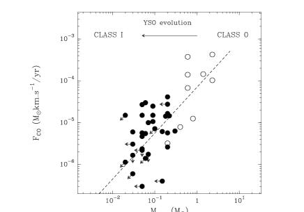
Figure 2: Outflow momentum flux $F_{\rm CO}$ versus circumstellar envelope mass $M_{\mbox{\tiny env}}$ for a sample of nearby Class I (filled circles) and Class 0 (open circles) YSOs (Bontemps et al. 1996). (The arrows on the data points indicate upper limits.) The ‘best fit’ $F_{\mbox{\tiny CO}}$–$M_{\mbox{\tiny env}}$ correlation is plotted as a dashed line. This diagram shows a clear decline of outflow power from Class 0s to Class Is.

In an effort to quantify this evolution of molecular outflows during the protostellar phase, Bontemps et al. (1996 – BATC) have recently obtained and analyzed a homogeneous set of CO(2–1) data around a large sample of low-luminosity ($L_{bol}<50\ L_{\odot}$), nearby ($d<450$ pc) embedded YSOs, including 36 Class I sources and 9 Class 0 sources. The results show that essentially all embedded YSOs have some degree of outflow activity, suggesting the outflow phase and the infall/accretion phase coincide. This is consistent with the idea that accretion cannot proceed without ejection and that outflows are directly powered by accretion (e.g., Ferreira & Pelletier 1995).
In addition, Class 0 objects are found to lie an order of magnitude above the well-known correlation between outflow momentum flux and bolometric luminosity holding for Class I sources. This confirms that Class 0 objects differ qualitatively from Class I sources, independently of inclination effects. On the other hand, as can be seen in Fig. 2, outflow momentum flux is roughly proportional to circumstellar envelope mass in the entire BATC sample (i.e., including both Class I and Class 0 sources). Bontemps et al. argue that this new correlation is independent of the $F_{\mbox{\tiny CO}}$–$L_{\mbox{\tiny bol}}$ correlation and most likely results from a progressive decrease of outflow power with time during the accretion phase.

Since many theoretical models of bipolar outflows (e.g. Shu et al. 1994, Ferreira & Pelletier 1995, Fiege & Henriksen 1996a,b) predict a direct proportionality between accretion and ejection, BATC further suggest that the observed decline in outflow power reflects a corresponding decrease in the mass accretion/infall rate: In this view, $\dot{M}_{\mbox{\tiny acc}}$ would decline from $\sim 10^{-5}\,\mbox{M${}_{\odot}\mbox{yr}^{-1}$}$ for the youngest Class 0 protostars to $\sim 10^{-7}\,\mbox{M${}_{\odot}\mbox{yr}^{-1}$}$ for the most evolved Class I sources and most active T Tauri stars.

3 Relevant theory

We propose that the decrease of accretion rate seen by BATC during the protostellar phase (see Sect. 2.2 above) is a direct consequence of the non-singular initial conditions indicated by the pre-stellar core observations summarized in Sect. 2.1. Our fundamental thesis in this article is that supersonic core formation and a subsequent core accretion flow may be adequately described as a zero pressure flow that evolves from a more general density profile than the $r^{-2}$ profile at a pre-core formation epoch ($t<0$). We use analytical methods to elucidate the physical origin of a sharp decrease of $\dot{M}_{\mbox{\tiny acc}}$ during the early accretion phase (i.e., just after the completion of stellar core formation). We show that the key to such a decrease is the existence of a transition between a flat inner region and an outer inverse square ‘envelope’ in the initial density profile: the inner region collapses first to form a hydrostatic stellar core, and the remaining cloud material then accretes supersonically onto a non-zero point mass.

3.1 Overview of known spherical collapse solutions

Here, we assemble some relevant non-linear studies of isothermal protostellar collapse in spherical geometry. The isothermality seems justified physically at early (e.g., pre-stellar) stages (note this does not imply the dynamical importance of pressure), but the assumption of spherical symmetry implies the neglect of rotation, magnetic fields and dynamical turbulence.

Mathematically, the paper by Whitworth & Summers (1985 – WS85) concludes the series of original studies on isothermal, self-similar accretion flows by Larson (1969), Penston (1969), Shu77 and Hunter (1977). However physically the debate continues, based essentially on the failure of either the Larson-Penston solution or the Shu solution to describe the accretion rate as found in numerical simulations (e.g. Hunter 1977, FC93) after the core-formation epoch. The Shu solution describes the asymptotic behaviour satisfactorily, while the Larson-Penston solution seems more relevant near core formation although it is not perfectly so.

The major contribution of WS85 was to show that a parametrically stable infinity of ‘acceptable’ similarity solutions exist rather than merely the previously known Larson-Penston (L/P) infall and the Shu (S) implosion behind an outward going expansion wave. ‘Acceptable’ in this context implies that the solutions have reasonable initial conditions inside an inward going compression wave in general (that may be initiated by an external disturbance) and describe supersonic infall after the passage of this wave. True free-fall accretion is established only after this wave has reached the centre of the system at $t=0$. It develops behind the rebounding expansion wave.

WS85 classified all possible isothermal similarity solutions in a bounded two-dimensional space. Briefly, this continuum of solutions spans a wide range from ‘gravity dominated’ solutions (corresponding to the ‘band 0/band 1’ of WS85) to ‘sound-wave’ dominated solutions (corresponding to high ‘band’ numbers in WS85). The sound-wave (or pressure) dominated solutions are those usually studied, which depend on the classical similarity variable $x=r/at$ (e.g., Shu77). The S solution is itself a limiting sound-wave dominated case (‘band $\infty$’ in WS85) that develops from an initial high density singular isothermal equilibrium.

One might think that the gravity dominated solutions should be determined in general by the form of the density or mass profile at some epoch in the region of supersonic flow, rather than by the isothermality as in the above family. We propose a more general type of similarity (see Appendix A and below) that arises from a given density profile in a region of supersonic flow. This idea was also hinted at in Hunter (1977) in the course of his explanation of the absence of shocks in the supersonic region prior to the arrival of the compression wave at $r=0$. Hunter observes that gravity provides a non-propagating local acceleration by ‘action at a distance’. Formally, the flow ceases to be hyperbolic in its causal structure, becoming elliptic instead.

Such a dynamical change in self-similar symmetry was considered by Henriksen (1994 – hereafter H94) to argue, on the basis of pressure-free, analytical calculations that non-constant accretion rates might be expected. We shall exploit this idea in the present paper after an assessment of the pressure dominated self-similar solutions.

It is difficult to isolate precisely the epoch at which the change in self-similarity type occurs. We know from the simulations by Hunter (1977) and recently by FC93 that classical self-similarity arises in the course of the collapse. The flow is generally found to agree best with the L/P type solution, but the agreement is not perfect, since the accretion rate found by these numerical studies is not the constant value to be expected if the self-similar solutions persist at the supersonic core formation epoch ($t=0$). In fact the accretion rate passes through a peak and then settles only gradually (if the cloud is sufficiently large) to the Shu value (see Fig. 3 of FC93). The nature of this transitory peak was left somewhat unclear by FC93 due to their problems of numerical resolution at $t=0$, but we believe its nature to be vital to the understanding of the outflow observations summarized in Sect. 2.2.

3.2 Justification of our pressure-free analytical approach

3.2.1 Neglect of magnetic field and rotation

We neglect both magnetic field and rotation in our discussion. Mouschovias and co-workers (Mouschovias 1995 and references therein) have demonstrated that a magnetically-supported, subcritical cloud evolves naturally to a centrally peaked, flattened density profile during a quasi-static phase of ambipolar diffusion. This mechanism can successfully account for the formation and structure of some isolated pre-stellar cores. The quasi-static phase ends with the formation of a magnetically supercritical core that collapses in a dynamical but magnetically-controlled fashion, while the bulk of the cloud remains magnetically supported. In Mouschovias’ models, the ‘dynamical’ contraction of the supercritical core is almost always subsonic and evolves only gradually towards free fall, which is not attained up to densities as large as $\sim 10^{9}$–$10^{10}$ cm^-3 (see Basu & Mouschovias 1995 and Fig. 2d of Ciolek & Mouschovias 1994). This corresponds to a rather gentle process of hydrostatic stellar core formation taking significantly longer than a free-fall time, i.e., typically on the order of $10^{6}$ yr in published models from the time the parent pre-stellar core becomes magnetically supercritical at a central density $\sim 10^{5}$ cm^-3.
However, as pointed out in Sect. 1 and Sect. 2.1, some cloud cores are apparently not magnetically supported and appear to evolve faster than predicted by ambipolar diffusion models. Furthermore, even in the case of initial magnetic support, superalfvénic implosion of cloud fragments is possible, for instance induced by a shock (e.g. Mouschovias 1989, Tomisaka, Ikeuchi, & Nakamura 1988, Tomisaka 1996). This may well be a dominant process in regions of multiple star formation. Thus, we believe the collapse can become vigorous and supersonic (superalfvénic as the case may be) relatively early on, at least in a small central mass (see the next section). This is the hypothesis we will make in the remainder of the paper.

Rotation and magnetic fields are thought to be essential to the launching of the bipolar outflows that are invariably found to be associated with protostars (e.g. Königl & Ruden 1993, Henriksen & Valls-Gabaud 1994). This argues in favour of their importance, at least when the outer parts of the initial cloud core fall in. It is likely that they are also important to the formation and evolution of the flattened inner parts.

Thus we cannot expect to include the whole picture self-consistently in our subsequent arguments which ignore magnetic fields. However if gravity is the main player in the core after a ‘point of no return’ is passed, then our present approach remains crudely justified, if incomplete.

3.2.2 Lagrangian treatment of Isothermal Self-Similarity

As discussed by Henriksen (1989 – H89), spherically symmetric, isothermal, self-similar collapse can be very conveniently treated when one uses a Lagrangian formalism. This is recalled briefly in Appendix A for the simplest cases. Here, we merely want to show that such a formalism provides continuity with the supersonic treatment to be found in Sect. 3.3. The advantage of the Lagrangian formulation is that self-similar solutions are fully described by the generalized ‘Friedmann, Lemaître, Robertson-Walker’ (FLRW) differential equation (Eq. A2 in the limit of Eqs. A4 and A5):

$$\left({dS\over d\xi}\right)^{2}-{1\over S}+\alpha_{s}^{2}H=k,$$

which expresses the conservation of energy. In this equation, $\xi\equiv\sqrt{2GM(r)/r^{3}}\,(t-t_{o})$ is the self-similar variable, where $M(r)$ is the mass distribution (i.e., the mass contained within the sphere of radius $r$ as a function of $r$) at some reference epoch $t=t_{o}$ (the reason for this time offset will become apparent later). The function $S(\xi)\equiv R(t,r)/r$ gives the normalized position at time $t$ of the shell that was initially ($t=t_{o}$) at $r$. Finally, $\alpha_{s}^{2}\equiv a_{s}^{2}r/GM(r)$ where $a_{s}$ is the isothermal sound speed, $H=\ln{\rho/\rho_{o}}$ where $\rho_{o}(r)$ is the density profile at $t=t_{o}$, and $k\equiv E(r)r/GM(r)=\pm 1$ or 0 is the normalized total energy ($E(r)$ being the specific total energy of the shell initially at $r$). The solutions describing a collapse from rest have $k=-1$, and those with zero total energy have $k=0$ (we omit other cases for simplicity).

The present formulation is unique in that it allows for a transition to a purely self-gravitating flow wherein the pressure is negligible (formally $\alpha_{s}\rightarrow 0$) before the ingoing compression wave establishes the $r^{-2}$ ‘attractor’ at $t=0$ [Blottiau, Bouquet, & Chièze (1988) were the first to use this terminology]. In order that $\alpha_{s}^{2}\rightarrow 0$ at $t<0$ in an isothermal flow, it is clear that $M(r)/r$ must tend to a large value as $r\rightarrow r_{N}$, where $r_{N}$ is the Lagrangian radius of this core or nuclear region. This can happen if a sufficiently dense mass with a flattened density profile forms at the centre of the system at $t<0$. This region should eventually collapse nearly homologously to form a central point mass so long as the inflow is supersonic (or super fast-Alfvénic as the case may be) and pressure support is negligible.

Assuming that some fraction of the core does collapse in the free-fall time $t_{ff}(N)$, we begin our zero pressure calculations at the onset of this rapid collapse. We define this starting point as being $t_{o}=-t_{ff}(N)$, for consistency with the standard pressure wave connected solutions. (With this definition, stellar core formation is complete at $t=0$, which also marks the beginning of the accretion phase.) When the parameter $\alpha_{s}^{2}\rightarrow 0$, one has made the transition of course from an hyperbolic system to an elliptic one. In other words, there is a wave-mitigated causality when pressure is important, and action at a distance (in Newtonian gravity) in the zero pressure limit (see also Hunter 1977). This is discussed briefly in Appendix A.

3.2.3 The case for starting from strictly flat inner density profiles

The density profiles observed in pre-stellar clouds (Sect. 2.1) are not as centrally flat as are some of the self-similar solutions of WS85, nor indeed of the magneto-static cores of Basu & Mouschovias (1995). This is not very surprising since a flat profile indicates a relatively low pressure gradient so that the hydrostatic equilibrium required for long lived clouds is not possible. In this state the cloud is in fact approaching the super-critical state. The real question then is whether the collapse proceeds in general by some part of the material passing through a phase of nearly zero pressure gradient and collapsing homologously, as the band 0 sound wave dominated self-similar solutions suggest (see Figs. 5, 6, 7 of WS85). Interestingly enough, the numerical calculations by FC93 that begin from non self-similar conditions show a velocity distribution in the critical Bonnor-Ebert sphere at early times that would tend to flatten the density profile (see e.g. the discussion in the second paragraph of their Sect. 2.3) while mildly sub-critical cases show oscillations as are found in the ‘bound’ (band 1 and higher) self-similar solutions. FC93 interpret their maximum velocity peak in terms of a flat interior density distribution that passes abruptly to a $r^{-2}$ profile. In fact, it is easy to show by linearizing the equations that an initially flattened density profile will first tend to evolve towards a still more flattened configuration on a free-fall timescale set by the cloud central density. Physically this is due once again to the velocity profile of the fastest growing linear mode that is consistent with zero velocity at the cloud edge and at the cloud centre, since this is such that the outer layers overtake the inner ones. The linear calculation can only be suggestive, but in the generalized solutions of Blottiau et al. (1988) as well as in the band 0 solutions of WS85, flattened centres and shells (which would also collapse to give a point mass) appear. Moreover during the ‘quasi-static’ evolution followed by Basu & Mouschovias (1995), flattened supercritical cores appear. That a portion of this core collapses homologously is however less clear from their calculations (depending on the ion-neutral collision time).

3.3 Accretion phase history

For the reasons given in Sect. 3.2 above, because of the nature of the abundant non-linear self-similar solutions (WS85), and because of the suggestive numerical study of FC93, we now proceed to calculate an accretion history for a self-similar cloud based on the following hypothesis of pre-collapse evolution.
In agreement with the observations, we suppose that the pre-collapse cloud core evolves quasi-statically, and develops a dense central region with a nearly flat density profile, until an external disturbance initiates the collapse. We further suppose that, after a transitional period (leading to, e.g., magnetic decoupling), the flat region is free to collapse suddenly, essentially homologously due to the absence of a pressure gradient. It is possible that further flattening of the profile occurs during the collapse. In any case the beginning of this free collapse is taken once again to be at $t=t_{o}\equiv-t_{ff}(N)$, so that the completion of the core collapse is at $t=0$, where $t_{ff}(N)$ is the free-fall time of a uniform sphere from rest, defined explicitly below. For all times $t>t_{o}$ we shall assume that the evolution is of the gravity-dominated self-similar form, given uniquely by the density profile at the $t=t_{o}$ epoch (see Appendix A). This is all that is required for the purposes of our calculation, but the flow has probably ceased to be pressure dominated even before $t=t_{o}$.
An important point to realize is that the accretion rate at $t=0$ will not yet be that appropriate to the exterior of the cloud, since this will be for some time dominated by the collapsed core mass rather than by the self-gravity appropriate to the outer density profile. The subsequent transition to a constant asymptotic accretion rate happens as sufficient mass from the outer cloud is accreted to dominate the initial core mass.

3.3.1 General Formulation

The equations include Eq. (1) above, plus those of Appendix A and of H89, H94 but with $\alpha_{s}^{2}=0$. We carry out the calculations for a family of initial density profiles which are all strictly flat for $r\leq r_{N}$ (see Fig. 3 below). The density is measured in units of the density $\rho_{N}$ of the flattened nucleus of the pre-collapse cloud (i.e., $\tilde{\rho}\equiv\rho/\rho_{N}$), the mass is in units of the mass nucleus $M_{N}$ (i.e., $\tilde{M}\equiv M/M_{N}$) and the radius is in units of $r_{N}$ (i.e., $\tilde{r}\equiv r/r_{N}$), where $r_{N}$ is the radius of the nuclear region just before free-fall collapse. For convenience, time is measured from the beginning of the free collapse ($t=t_{o}=-t_{ff}(N)$) in units of the nuclear region free-fall time $t_{ff}(N)=(3\pi/32G\rho_{N})^{1/2}$, that is we introduce the dimensionless variable

$$\tau\equiv{t-t_{o}\over t_{ff}(N)}.$$

The stellar core is fully formed at $\tau=1$ and consists of all shells with Lagrangian labels $\tilde{r}\leq 1$. We take this epoch to correspond to $\xi=\pi/2$ since this is appropriate to the collapse of a uniform sphere from rest (e.g. Hunter 1962). In this description, $\tau=1$ also marks the beginning of the YSO accretion phase, while dimensionless times in the range $0<\tau<1$ correspond to ‘isothermal protostars’ (i.e., collapsing cloud fragments with no central hydrostatic core – see Sect. 1).
The introduction of the self-similar variable $\xi$ ($0\leq\xi\leq\pi/2$) is partly justified by the fact that the free-fall time of the shell with Lagrangian label $\tilde{r}$ is related to the mass function $M(r)$ through

$$t_{ff}(\tilde{r})=\sqrt{\tilde{r}^{3}\over\tilde{M}(\tilde{r})}\,t_{ff}(N)=({\pi/2\over\xi})\,(t-t_{o}).$$

Thus, for $\tilde{r}\geq 1$ we have $\xi\leq\pi/2$ and

$${\xi\over\pi/2}=\tau\,\sqrt{\tilde{M}(\tilde{r})\over\tilde{r}^{3}}.$$

(In the post nuclear formation epoch, we have $\xi=\pi/2$ for all $\tilde{r}\leq 1$ since these shells have already collapsed in the singular nucleus.)

We shall be interested in those shells which are accreting near the center during the post nuclear formation phase and thus which are about to enter the singularity. As is well known in cosmology (FLRW models, see H89), for such shells a collapse in the absence of significant pressure gradients can be described by Eq. (1) with $k=0$ (and $\alpha_{s}^{2}=0$), for which the solution is

$$S(\xi)=\left({3\over 2}({\pi\over 2}-\xi)\right)^{2/3},$$

for $\xi\leq\pi/2$.

We note immediately that $\tau=1$ when $\xi=\pi/2$ for the outer shell of the nucleus ($\tilde{r}=1$), which is the instant when the nucleus has fully formed.

To obtain the relationship between the real position of a spherical shell $R(\tau,r)$ and its Lagrangian or comoving label $r$ we must use $R=rS(\xi)$, which with Eq. (4) gives

$${\xi\over\pi/2}=-{4\over 3\pi}\left({R\over r}\right)^{3/2}+1.$$

We see that $R=0$ when $\xi=\pi/2$ as expected. Note however that nevertheless the shell label $\tilde{r}$ will be greater than or equal to $1$ in our calculations, since we shall be studying spheres whose initial radii are greater than or equal to $r_{N}$.

Our goal is to calculate the accretion rate history and the mass remaining in the envelope surrounding the collapsed nucleus, since both of these quantities are susceptible to observation. The accretion rate $\dot{M}_{\mbox{\tiny acc}}$ is given at each spherical radius $R$ and time $t$ by $\mbox{$\dot{M}_{\mbox{\tiny acc}}$}=4\pi R^{2}\,\rho\,\partial_{t}R$. If we use our various definitions and measure distance and density in units as above, and velocity in units of the nuclear free-fall velocity $v_{N}\equiv\sqrt{2GM_{N}/r_{N}}$ we obtain

$$\dot{\tilde{M}}_{acc}\equiv{\mbox{$\dot{M}_{\mbox{\tiny acc}}$}\over 4\pi r_{N}^{2}\rho_{N}v_{N}}=\tilde{r}^{2}\tilde{\rho}S^{2}\,{dS\over d\xi}\,\sqrt{\tilde{M}(\tilde{r})\over\tilde{r}},$$

where $S$ is given by Eq. (4) and $\tilde{\rho}$ follows from Eq. (A3) in the form

$$\tilde{\rho}={\tilde{\rho}_{o}(r)\over S^{3}(1+{d\ln S\over d\ln\xi}{\partial\ln\xi\over\partial\ln r})},$$

where $\rho_{o}$ is the density profile at $t=t_{o}$.

Since we are mainly interested in calculating the accretion rate near the centre of the post-collapse configuration where $R/r\rightarrow 0$, we may let $\xi$ tend towards $\xi=\pi/2$ in Eq. (6).

The mass $M_{\star}$ of the central collapsed object accreting the shell labelled $\tilde{r}$ at the time $\tau$ is also easily obtained by setting $\xi=\pi/2$ in Eq. (3) :

$$\tilde{M}_{\star}(\tau)={\tilde{r}^{3}(\tau)\over\tau^{2}}.$$

It is perhaps worth repeating this equation in the form that it assumes with restored dimensions, namely

$$M_{\star}(t)={\pi^{2}\over 8}~{}{r^{3}(t)\over G(t-t_{o})^{2}}.$$

Conversely, the time at which the shell initially at $\tilde{r}$ accretes onto the central singularity is

$$\tau=\sqrt{{\tilde{r}^{3}\over\tilde{M}(\tilde{r})}}.$$

As for the total mass of the accreting circumstellar envelope at time $\tau$, it is simply $\tilde{M}_{env}(\tau)\equiv\tilde{M}_{cloud}-\tilde{M}_{\star}(\tau)$.

3.3.2 Two-component Power-Law Model

To obtain explicit expressions for $\dot{M}_{\mbox{\tiny acc}}$ and $M_{env}$, we must assume an explicit initial density profile. We use a multi-component profile of the form (in the units introduced in Sect. 3.3.1)

$$\tilde{\rho_{o}}=\tilde{r}^{-2/D_{1}},~{}~{}1\leq\tilde{r}<\tilde{r}_{b},$$

$$\tilde{\rho_{o}}=\tilde{r_{b}}^{-2/D_{1}}\,({\tilde{r}\over\tilde{r_{b}}})^{-2/D_{2}},~{}~{}\tilde{r}\geq\tilde{r_{b}},$$

and $\tilde{\rho_{o}}=1$ for $\tilde{r}\leq 1$, where $\tilde{r}_{b}$ is a characteristic boundary radius, $D_{1}$ is a positive number characterizing the power-law slope of the cloud ‘envelope’, and $0<D_{2}<2/3$ characterizes the radial profile of the ‘edge’ of the model pre-stellar core (see Fig. 3). This form gives a weak discontinuity in the density profile between the flat nucleus and the $r^{-2/D_{1}}$ envelope (the density remains continuous but its derivative is discontinuous at $r=r_{N}$). This discontinuity breaks the density self-similarity but not the dynamical self-similarity as discussed in H89. In a pressure-free epoch there is no reason why such a discontinuity might not be preserved, if ever it were to be established by an inward propagating wave for example. Such weak discontinuities often arise during the adjustment of a gas to a change in the boundary conditions (e.g. Landau & Lifshitz 1987) and this may well be the manner in which the collapse is initiated. In this subsection, we will keep $D_{1}$ and $D_{2}$ as free parameters in order to obtain general formulae and model a wide range of accretion histories, but in practice we will use $D_{1}=1$ ($r^{-2}$ envelope) and $D_{2}=0.1$ when comparing with observations (Sect. 4). The rationale behind such a two-component, idealized density profile is that it approximates the observed structure of pre-stellar cores reasonably well (cf. WSHA, AWM96, Abergel et al. 1996, and Sect. 2.1) and can account for the necessarily finite radius of influence of protostars forming in clusters (since $D_{2}<2/3$ the model pre-stellar core has a steep edge and a finite total mass, see below).

Figure 3: Density $vs.$ radius (in log–log format) for an idealized pre-stellar cloud with a flat nucleus surrounded by a power-law envelope and a steeper power-law outer boundary

With this density profile, the mass function $M(r)$ that appears in the self-similar variable $\xi$ (see Appendix A and H89) in the post ‘nuclear collapse’ domain ($\xi>0$) is $\int_{r_{N}}^{r}\,\rho_{o}dr+M_{N}$, where the nuclear mass is $M_{N}=(4\pi/3)\rho_{N}r_{N}^{3}$. Thus, the mass distribution in units of $M_{N}$ takes the simple form

$$\tilde{M}(\tilde{r})=(3D_{1}\tilde{r}^{(3-2/D_{1})}-2)/(3D_{1}-2),~{}~{}~{}~{}1\leq\tilde{r}<\tilde{r}_{b},$$

$$\tilde{M}(\tilde{r})=\tilde{M}_{b}+{3D_{2}\tilde{r}_{b}^{(3-2/D_{1})}\over 3D_{2}-2}\,[({\tilde{r}\over\tilde{r}_{b}})^{(3-2/D_{2})}-1],~{}~{}~{}~{}\tilde{r}\geq\tilde{r_{b}},$$

where $\tilde{M}_{b}=(3D_{1}\tilde{r}_{b}^{(3-2/D_{1})}-2)/(3D_{1}-2)$ is the mass enclosed within the boundary radius $\tilde{r}_{b}$. Since $D_{2}<2/3$, the mass function converges at large $\tilde{r}$ towards $\tilde{M}_{cloud}=\tilde{M}_{b}+[3D_{2}\tilde{r}_{b}^{(3-2/D_{1})}/(2-3D_{2})]$. (Note that the case $D_{2}=2/3$, which we do not include explicitly here, is logarithmic.)

In this case, the time function $\tau(\tilde{r})$ giving the time of arrival in the central hydrostatic core of the shell initially at $\tilde{r}$ (see Eq. 8) can be easily inverted and has simple power-law asymptotic forms: $\tilde{r}(\tau)\sim({3D_{1}\over 3D_{1}-2})^{D_{1}/2}\times\tau^{D_{1}}$ before accretion of the shell labeled $\tilde{r}_{b}$, and
$\tilde{r}(\tau)\sim\tilde{M}_{cloud}^{1/3}\times\tau^{2/3}$ at later times. Figure 4 displays this $\tilde{r}(\tau)$ relationship for three initial density profiles which all have a sharp outer boundary ($\tilde{r}_{b}=10$ and $D_{2}=0.1$).

Figure 4: Radius of the shell accreting onto the central singularity as a function of time for three values of $D_{1}$ corresponding to $r^{-1}$ (dotted curve), $r^{-2}$ (solid curve), and $r^{-3}$ (dash-dotted curve) envelopes respectively in the initial density profile. A sharp outer edge ($\tilde{r}_{b}=10$ and $D_{2}=0.1$) has been assumed in all three cases. The dashed line shows the linear relation $\tilde{r}=3^{1/2}\tau$ expected for a singular $r^{-2}$ sphere. By definition, $\tau=1$ corresponds to the time at which the outer shell of the flat nucleus reaches the central singularity

The special $D_{1}=1$ case ($r^{-2}$ ‘envelope’, which we will use in practice) is particularly instructive since it shows that a singular $r^{-2}$ pre-stellar core would collapse according to the linear relation $\tilde{r}=\sqrt{3}\,\tau$ or $r(t)={2\sqrt{3}\over\pi}\,v_{N}\,(t-t_{o})$ in restored dimensions. This makes possible a direct comparison with Shu77’s expansion wave solution which predicts $r(t)=R_{inf}/2=(a_{s}/2)\,t$ (here $R_{inf}$ denotes the head of the expansion wave at time $t$; note that $t_{o}=0$ in Shu’s solution). In a sense, Fig. 4 illustrates that, during the accretion phase, the idealized solutions explored in this paper are characterized by an ‘inside-out’ collapse behind an expansion wave reminiscent of the Shu solution.

Figure 5: Accretion rate as a function of time for three values of $D_{1}$ corresponding to $r^{-1}$ (dotted curve), $r^{-2}$ (solid curve), and $r^{-3}$ (dash-dotted curve) envelopes respectively in the initial density profile. A sharp outer edge ($\tilde{r}_{b}=10$ and $D_{2}=0.1$) has been assumed in all three cases. The dashed horizontal line gives the asymptotic value of the accretion rate obtained in the case an $r^{-2}$ initial density profile

Substituting Eqs. (10) and (10’) into Eq (6), we obtain the desired accretion rate history at $\xi=\pi/2$ explicitly as

$$\dot{\tilde{M}}_{acc}=-({2\over 3\pi}){\tilde{r}^{(3-2/D_{1})}\over\tau}\,{3D_{1}\tilde{r}^{(3-2/D_{1})}-2\over\tilde{r}^{(3-2/D_{1})}-1},$$

as long as the expansion wave is still within $\tilde{r}_{b}$. At later times, the accretion history may be obtained from the relation:

$$\dot{\tilde{M}}_{acc}=-({4\over 3\pi}){\tilde{r}_{b}^{2/\bar{D}}\tilde{r}^{(3-2/D_{2})}\over\tau}\,{\tilde{M}(\tilde{r})\over\tilde{M}(\tilde{r})-\tilde{r}_{b}^{2/\bar{D}}\tilde{r}^{(3-2/D_{2})}},$$

where $\bar{D}$ is defined by $1/\bar{D}\equiv(1/D_{2})-(1/D_{1})$. Based on these formulae, Fig. 5 displays the predicted accretion rate as a function of time for the same three model pre-stellar profiles as in Fig. 4.

Figure 6: Absolute value of the accretion rate as a function of envelope mass for the same three initial density profiles as in Fig. 4 and Fig. 5. Here again, the dashed horizontal line gives the asymptotic value of the accretion rate predicted in the case an $r^{-2}$ initial density profile

The corresponding relationships between $\dot{\tilde{M}}_{acc}$ and $\tilde{M}_{env}$ are shown in Fig. 6.

Equation (11) implies that the accretion rate diverges at $\tilde{r}=1$ (i.e., $\tau=1$) and asymptotically approaches a power-law dependence at large $\tilde{r}$ (i.e., large $\tau$), $\dot{\tilde{M}}_{acc}\propto\tau^{(3D_{1}-3)}$ if $D_{1}>2/3$, and $\dot{\tilde{M}}_{acc}\propto\tau^{(3D_{1}-4/3D_{1})}$ if $D_{1}<2/3$ (see Fig. 5). (Here again, the case $D_{1}=2/3$ is logarithmic.) In particular, $\dot{\tilde{M}}_{acc}$ tends to the asymptotic value $-\sqrt{3}.(2/\pi)$ at large $\tau$ when $D_{1}=1$ ($r^{-2}$ envelope) (see also Appendix B). As was observed by H94 and FC93, this asymptotic limit is only achieved if the envelope is sufficiently large (i.e., typically $\tilde{r}_{b}\lower 2.15277pt\hbox{$\;\buildrel>\over{\sim}\;$}4$). Otherwise the accretion rate associated with stellar formation is truncated abruptly as the surface of the protostellar cloud falls in. Terminal accretion may continue after this stage as noted in H94 but with a character that depends on the density profile in the environment. We try to simulate this late effect here with a steep $D_{2}=0.1$ edge (see Eq. 9’).
The accretion peak at $\tau=1$ is due to the close approach of the density profile to being flat near $\tilde{r}=1$. Physically, if the density profile is strictly flat, two distinct spherical shells fall to the centre simultaneously, so that the frequency of shell arrival (which is the accretion rate) is infinite. It is in fact easy to show from the preceding theory that the criterion for a shell at $r$ and another at $r+\delta r$ to be accreted at $R=0$ at a transitory peak rate is indeed that

$${d\ln{M(r)}\over d\ln{r}}\rightarrow 3.$$

In fact, if the density profile is not perfectly flat at some point $r_{N}$, e.g., $\rho_{o}\propto r^{-2\epsilon}$ locally where $\epsilon$ is small and positive, then the logarithmic derivative of Eq. (12) attains the value $3-2\epsilon$, and one finds that the accretion rate for these shells will have a peak amplitude (in the usual units at $r_{N}$)

$$\dot{\tilde{M}}_{acc}^{peak}=-{2\over\pi\epsilon}.$$

4 Discussion: Implications for protostellar evolution

What we should retain from the previous analytical calculations is the association of centrally peaked, flattened, pre-stellar density profiles with a transitory, vigorous, post nuclear formation accretion epoch. We here suggest that this energetic accretion phase coincides with Class $0$ protostars, which would explain their unusually powerful jets compared to the more evolved Class I YSOs (see Sect. 2.2).

4.1 Predicted versus observed accretion histories

We proceed to compare the model predictions obtained in Sect. 3.3 above with the $\mbox{$F_{\mbox{\tiny CO}}$}\,c/\mbox{$L_{\mbox{\tiny bol}}$}$ versus $\mbox{$M_{\mbox{\tiny env}}$}/\mbox{$L_{\mbox{\tiny bol}}$}^{0.6}$ diagram corresponding to the entire BATC sample. This diagram, which is almost free of any luminosity or distance effect, should mainly reflect the evolution of the accretion rate $\dot{M}_{\mbox{\tiny acc}}$. Indeed, as discussed by AWB93 and BATC, the $\mbox{$M_{\mbox{\tiny env}}$}/\mbox{$L_{\mbox{\tiny bol}}$}^{0.6}$ ratio can be used as a practical, quantitative indicator of embedded YSO evolution, which, to first order, should track the ratio $\mbox{$M_{\mbox{\tiny env}}$}/\mbox{$M_{\mbox{\tiny$\star$}}$}$ of envelope to stellar mass and thus decrease with protostellar age. As to the CO outflow momentum flux $F_{\mbox{\tiny CO}}$, it is related to the accretion rate $\dot{M}_{\mbox{\tiny acc}}$ by

$$\mbox{$F_{\mbox{\tiny CO}}$}=[\mbox{$f_{\mbox{\tiny ent}}$}\,(\mbox{$\dot{M}_{\mbox{\tiny w}}$}/\mbox{$\dot{M}_{\mbox{\tiny acc}}$})\,\mbox{$V_{\mbox{\tiny w}}$}]\times\mbox{$\dot{M}_{\mbox{\tiny acc}}$},$$

where $f_{\mbox{\tiny ent}}$ is the entrainment efficiency, $\dot{M}_{\mbox{\tiny w}}$ is the mass-loss rate of the underlying driving wind or jet, and $V_{\mbox{\tiny w}}$ is the wind velocity. As discussed in BATC, $\mbox{$f_{\mbox{\tiny ent}}$}\,(\mbox{$\dot{M}_{\mbox{\tiny w}}$}/\mbox{$\dot{M}_{\mbox{\tiny acc}}$})\,\mbox{$V_{\mbox{\tiny w}}$}$ is unlikely to vary much during the protostellar phase, so that $F_{\mbox{\tiny CO}}$ should reflect the variations of the accretion rate $\dot{M}_{\mbox{\tiny acc}}$. However, because as a general trend more massive cores tend to form more massive and more luminous YSOs associated with more energetic outflows (e.g. Saraceno et al. 1996), $F_{\mbox{\tiny CO}}$ also depends on luminosity or stellar mass. For this reason, we use the quantity $\mbox{$F_{\mbox{\tiny CO}}$}\,c/\mbox{$L_{\mbox{\tiny bol}}$}$ instead which should be less sensitive to the initial cloud mass/density. To the extent that there is no significant luminosity evolution for a given protostellar source (see Kenyon & Hartmann 1995 and BATC), $\mbox{$F_{\mbox{\tiny CO}}$}\,c/\mbox{$L_{\mbox{\tiny bol}}$}$ should more homogeneously trace the intrinsic temporal variations of $\dot{M}_{\mbox{\tiny acc}}$ than $F_{\mbox{\tiny CO}}$.

The $\mbox{$F_{\mbox{\tiny CO}}$}\,c/\mbox{$L_{\mbox{\tiny bol}}$}$ versus $\mbox{$M_{\mbox{\tiny env}}$}/\mbox{$L_{\mbox{\tiny bol}}$}^{0.6}$ diagram observed by BATC, which is shown in Fig. 7, suggests that the accretion rate of Class 0 sources is a factor of $\sim 10$ larger on average than that of Class I sources (see also Sect. 4.3.1 of BATC). By comparison with Fig. 6, it is tempting to identify the Class 0 phase with the short period of vigorous accretion predicted by the theory of Sect. 3.3 after the formation of the hydrostatic stellar nucleus, and the Class I phase with the longer period of constant $\dot{M}_{\mbox{\tiny acc}}$ predicted at late times when $D_{1}=1$ ($r^{-2}$ envelope).

Figure 7: $\mbox{$F_{\mbox{\tiny CO}}$}\,\mbox{c}/\mbox{$L_{\mbox{\tiny bol}}$}$ (dimensionless) versus $\mbox{$M_{\mbox{\tiny env}}$}/\mbox{$L_{\mbox{\tiny bol}}$}^{0.6}$ ($M_{\mbox{\tiny env}}$ and $L_{\mbox{\tiny bol}}$ in units of M_⊙ and L_⊙) for the sample of Class 0 (open circles) and Class I (filled circles) sources studied by Bontemps et al. (1996). (The arrows on the data points indicate upper limits.) $\mbox{$F_{\mbox{\tiny CO}}$}\,\mbox{c}/\mbox{$L_{\mbox{\tiny bol}}$}$ can be taken as an empirical tracer of $\dot{M}_{\mbox{\tiny acc}}$ provided that there is no significant luminosity evolution. $\mbox{$M_{\mbox{\tiny env}}$}/\mbox{$L_{\mbox{\tiny bol}}$}^{0.6}$ is an evolutionary indicator which decreases with protostellar age. The eye-fitted solid curve shows the accretion rate history predicted by the model of Sect. 3.3.2 assuming $D_{1}=1$, $D_{2}=0.1$, and $\tilde{r}_{b}=1.6$ (see text). The dashed line shows the corresponding asymptotic value of $\mbox{$F_{\mbox{\tiny CO}}$}\,\mbox{c}/\mbox{$L_{\mbox{\tiny bol}}$}$ for comparison with Fig. 5 and Fig. 6.

To make quantitative comparisons, we use an independent observational constraint on the average values of the accretion rate during the Class I and Class 0 phases. The lifetime of Class I sources is measured to be $\Delta t_{I}\sim 2\times 10^{5}$ yr in clouds forming mainly low-mass stars such as $\rho$ Ophiuchi and Taurus (e.g. Wilking et al. 1989, Kenyon et al. 1990, Greene et al. 1994). The lifetime of Class 0 sources is estimated to be an order of magnitude shorter, $\Delta t_{0}\lower 2.15277pt\hbox{$\;\buildrel>\over{\sim}\;$}10^{4}$ yr (see AM94 and Barsony 1994). In this paper, we adopt the conceptual definitions of the Class 0 and Class I stages introduced by AWB93 (see also AM94). The Class 0 stage corresponds to protostars which have developed a hydrostatic stellar core but still have $\mbox{$M_{\mbox{\tiny env}}$}>\mbox{$M_{\mbox{\tiny$\star$}}$}$, i.e., objects which have accreted less than a half of the total cloud mass; in our model, the formation of the central hydrostatic object ends when the flat pre-stellar nucleus has fully collapsed, thus Class 0 sources have $M_{N}<\mbox{$M_{\mbox{\tiny$\star$}}$}<M_{cloud}/2$. The Class I stage corresponds to embedded sources with smaller envelope masses: $\mbox{$M_{\mbox{\tiny env}}$}<\mbox{$M_{\mbox{\tiny$\star$}}$}$. We also define the boundary between Class I and Class II sources by $\mbox{$M_{\mbox{\tiny$\star$}}$}=0.99\times M_{cloud}$, i.e., $\mbox{$M_{\mbox{\tiny env}}$}=0.01\times M_{cloud}$. This allows for residual (disk) accretion during the (Class II) pre-main sequence phase: a $1\ \mbox{M${}_{\odot}$}$ star may typically accrete up to the mass of the minimum solar nebula, i.e., $0.01\ \mbox{M${}_{\odot}$}$, at the Class II stage ($0.01\ \mbox{M${}_{\odot}$}$ is indeed the median circumstellar disk mass measured around Class II T Tauri stars – Beckwith et al. 1990, AM94).

Within the framework of the model introduced in Sect. 3.3.2 the mass function $\tilde{M}(\tilde{r})$ is easy to invert, and given the above definitions the lifetime ratio $\Delta t_{I}/\Delta t_{0}$ can be calculated analytically as a function of $\tilde{M}_{cloud}$ or $\tilde{r}_{b}$:

$$\Delta t_{I}/\Delta t_{0}=(\tau_{I}-\tau_{0})/(\tau_{0}-1),$$

where

$$\tau_{0}=[\tilde{r}(\tilde{M}_{cloud}/2)]^{3/2}/(\tilde{M}_{cloud}/2)^{1/2},$$

and

$$\tau_{I}=[\tilde{r}(0.99\tilde{M}_{cloud})]^{3/2}/(0.99\tilde{M}_{cloud})^{1/2}.$$

This model ratio is plotted in Fig. 8 as a function of the boundary radius $\tilde{r}_{b}$, for the same three values of $D_{1}$ as in Figs. 4, 5, 6.

Figure 8: Predicted ratio of the duration of the Class I phase $\Delta t_{I}$ to the duration of the Class 0 phase $\Delta t_{0}$ as a function of the pre-stellar boundary radius $\tilde{r}_{b}$ within the model of Sect. 3.3.2 (see text for formal definitions of the Class 0 and Class I phases). Three representative cases are shown: $r^{-1}$ envelope ($D_{1}=2$, dotted curve), $r^{-2}$ envelope ($D_{1}=1$, solid curve), $r^{-3}$ envelope ($D_{1}=2/3$, dash-dotted curve). In all three cases, a sharp outer boundary ($D_{2}=0.1$) has been assumed beyond $\tilde{r}_{b}$.

It can be seen from Fig. 8 that the observational constraint $\Delta t_{I}/\Delta t_{0}\sim 10$ can be satisfied by the $D_{1}=1$ model (standard case) only if the pre-stellar boundary radius is small ($\tilde{r}_{b}\sim 1.6$), corresponding to a small value of the normalized cloud mass ($\tilde{M}_{cloud}\sim 3$). Furthermore, the predicted $\Delta t_{I}/\Delta t_{0}$ ratio decreases rapidly towards an asymptotic value of 1 as $\tilde{r}_{b}$ increases (one already has $\Delta t_{I}/\Delta t_{0}\lower 2.15277pt\hbox{$\;\buildrel<\over{\sim}\;$}2$ for $\tilde{r}_{b}=3.5$, i.e., $\tilde{M}_{cloud}\sim 9$). The $D_{1}=2$ case is qualitatively similar. In contrast, for sharper initial density profiles such as $r^{-3}$ ($D_{1}=2/3$), the predicted lifetime ratio $\Delta t_{I}/\Delta t_{0}$ is $\lower 2.15277pt\hbox{$\;\buildrel>\over{\sim}\;$}10$ for a wide range of $\tilde{r}_{b}$ values.

Since the mean stellar mass in the BATC sample is $<M_{\star}>\lower 2.15277pt\hbox{$\;\buildrel<\over{\sim}\;$}1\ \mbox{M${}_{\odot}$}$, the average accretion rate during the Class I phase can be estimated as
$<\mbox{$\dot{M}_{\mbox{\tiny acc}}$}>_{I}\,\approx\,<M_{\star}>/(2\Delta t_{I})\sim 2.5\times 10^{-6}\ \mbox{M${}_{\odot}\mbox{yr}^{-1}$}$. In addition, one has

$$<\mbox{$\dot{M}_{\mbox{\tiny acc}}$}>_{0}/<\mbox{$\dot{M}_{\mbox{\tiny acc}}$}>_{I}\,\approx\,\Delta t_{I}/\Delta t_{0}\times(1-\frac{2}{\tilde{M}_{cloud}}).$$

Therefore, if $\tilde{M}_{cloud}$ is sufficiently larger than 2, the lifetime constraint $\Delta t_{I}/\Delta t_{0}\sim 10$ implies
$<\mbox{$\dot{M}_{\mbox{\tiny acc}}$}>_{0}/<\mbox{$\dot{M}_{\mbox{\tiny acc}}$}>_{I}\,\sim 10$, in reasonable agreement with the drop of $\mbox{$F_{\mbox{\tiny CO}}$}\,c/\mbox{$L_{\mbox{\tiny bol}}$}$ seen in Fig. 7 between Class 0s and Class Is.

To reduce the number of free parameters, we will assume $D_{1}=1$ and $D_{2}=0.1$ from now on. With these values, the model profile accounts for the nearly $r^{-2}$ ‘envelope’ that is observed in most pre-stellar cores just outside the flat central region (WSHA, AWM96). It also features a steep outer edge, qualitatively similar to those revealed by some recent infrared absorption studies of dense cores (Dent et al. 1995, Abergel et al. 1996).
The boundary radius $\tilde{r}_{b}$ is the only parameter of the model that we will vary in order to match the observations. As discussed above, the lifetime constraint suggests $\tilde{r}_{b}\sim 1.6$. In Fig. 7, we have superposed as a solid curve the accretion history predicted by the model when $\tilde{r}_{b}=1.6$ (and $D_{1}=1$, $D_{2}=0.1$) to the $\mbox{$F_{\mbox{\tiny CO}}$}\,c/\mbox{$L_{\mbox{\tiny bol}}$}$ versus $\mbox{$M_{\mbox{\tiny env}}$}/\mbox{$L_{\mbox{\tiny bol}}$}^{0.6}$ diagram observed by BATC. To scale the model along the x-axis, we adopted $M_{cloud}=1\ \mbox{M${}_{\odot}$}$, based on the average value of $M_{\mbox{\tiny env}}$ for the Class 0 sources in the BATC sample. The outflow efficiency factor $\mbox{$f_{\mbox{\tiny ent}}$}\,(\mbox{$\dot{M}_{\mbox{\tiny w}}$}/\mbox{$\dot{M}_{\mbox{\tiny acc}}$})\,\mbox{$V_{\mbox{\tiny w}}$}$ was adjusted so as to make the model match the typical value $\mbox{$F_{\mbox{\tiny CO}}$}\,\mbox{c}/\mbox{$L_{\mbox{\tiny bol}}$}\sim 200$ observed among the Class I sources of the BATC sample. Given an average bolometric luminosity $<\mbox{$L_{\mbox{\tiny bol}}$}>\,=2\ \mbox{L${}_{\odot}$}$ (BATC), this corresponds to a typical momentum flux $<\mbox{$F_{\mbox{\tiny CO}}$}>\,\sim 8\times 10^{-6}\,\mbox{M${}_{\odot}\mbox{km s}^{-1}\mbox{yr}^{-1}$}$ for Class I sources. At late times the ($D_{1}=1$) model predicts a constant accretion rate $M_{acc}^{0}$ corresponding to the standard Shu value (see Appendix B). If we adopt $M_{acc}^{0}\sim 2\times 10^{-6}\,\mbox{M${}_{\odot}\mbox{yr}^{-1}$}$, which is appropriate for a $T=10$ K cloud and in rough agreement with the value estimated above from the lifetime of Class I sources, then we find that the best ‘eye-fit’ model has an efficiency $\mbox{$f_{\mbox{\tiny ent}}$}\,(\mbox{$\dot{M}_{\mbox{\tiny w}}$}/\mbox{$\dot{M}_{\mbox{\tiny acc}}$})\,\mbox{$V_{\mbox{\tiny w}}$}\sim 4\,\mbox{km s${}^{-1}$}$. We note that this is a factor of 4 lower than the efficiency used in BATC which corresponds to the canonical values $\mbox{$V_{\mbox{\tiny w}}$}=150\,\mbox{km s${}^{-1}$}$, $\mbox{$\dot{M}_{\mbox{\tiny w}}$}/\mbox{$\dot{M}_{\mbox{\tiny acc}}$}=0.1$, and $\mbox{$f_{\mbox{\tiny ent}}$}=1$. A possible explanation for this difference is that the entrainment efficiency is actually lower than 1, $\mbox{$f_{\mbox{\tiny ent}}$}\sim 0.25$. In spite of this discrepancy, the overall agreement between the shape of the predicted accretion history and the observations is quite encouraging given the simplicity of the present modeling. In particular, it should be noted that the range of initial $M_{cloud}$ values spanned by the BATC sample is certainly only partly accounted for by dividing $F_{\mbox{\tiny CO}}$ by $L_{\mbox{\tiny bol}}$ and plotting $\mbox{$F_{\mbox{\tiny CO}}$}\,c/\mbox{$L_{\mbox{\tiny bol}}$}$ versus $\mbox{$M_{\mbox{\tiny env}}$}/\mbox{$L_{\mbox{\tiny bol}}$}^{0.6}$.

A potential problem of the $D_{1}=1$ model shown in Fig. 7 is that it apparently leads to very short timescales. For $\tilde{r}_{b}=1.6$, the predicted Class 0 and Class I lifetimes are indeed $\Delta t_{0}\sim 0.04\,t_{ff}(N)$ and $\Delta t_{I}\sim 0.37\,t_{ff}(N)$ in units of the nuclear region free-fall time. If we take the mean density $n_{H_{2}}\sim 2\times 10^{5}$ cm^-3 observed in the flat central region of L1689B (AWM96) as a representative example, we obtain $t_{ff}(N)\sim 7\times 10^{4}$ yr, and thus $\Delta t_{0}\sim 2500$ yr and $\Delta t_{I}\sim 2.6\times 10^{4}$ yr, which are at least a factor of $\sim 4$ shorter than the observed values of $\Delta t_{0}$ and $\Delta t_{I}$.
However, in actual fact, the collapse is probably less violent than indicated by our self-similar, pressure-less calculations. The more realistic numerical calculations of FC93 and Tomisaka (1996), which fully account for pressure support (including magnetic support in the latter case), yield qualitatively similar accretion histories but quantitatively longer timescales. In particular, the core formation time since the initiation of collapse is a factor of $\sim 4$–$5$ times larger than the free-fall time $t_{ff}(N)$ in these calculations. If we use this factor to roughly estimate the slowing down influence of pressure effects, then we find $\Delta t_{0}\sim 10^{4}$ yr and $\Delta t_{I}\sim 10^{5}$ yr, in better agreement with the observed lifetimes.

4.2 Accretion luminosities of Class 0 and Class I sources

If, as proposed here, $\dot{M}_{\mbox{\tiny acc}}$ is a factor of $\sim 10$ larger for Class 0 sources than for Class I sources, one may naively expect the former to have much higher accretion luminosities than the latter. This would be in apparent contradiction with observations which suggest that Class 0s are not significantly over-luminous compared to Class Is. For instance, in the embedded YSO sample of BATC, the ratio of the average bolometric luminosities for the two classes was $<\mbox{$L_{\mbox{\tiny bol}}$}>_{0}/<\mbox{$L_{\mbox{\tiny bol}}$}>_{I}\sim 1.6$. (Note however that the typical luminosity of Class 0 sources in a given cloud is relatively uncertain observationally due to the rarity of these objects.)

In reality, several factors contribute to reduce the theoretical accretion luminosity (L${}_{acc}=GM_{\star}\dot{M}_{acc}/R_{\star}$) at the Class 0 stage, making it comparable to the Class I accretion luminosity:
(1) The central stellar mass $M_{\star}$ is smaller for Class 0 sources;
(2) The stellar radius $R_{\star}$ is likely to be larger if $\dot{M}_{\mbox{\tiny acc}}$ is higher, since one expects the rough scaling $R_{\star}\propto\mbox{$\dot{M}_{\mbox{\tiny acc}}$}^{1/3}$ (Stahler, Shu, & Taam 1980; Stahler 1988);
(3) The amount of accretion energy dissipated in the wind can be expected to be larger for Class 0s than for Class Is (and could be a significant fraction of the total accretion energy).

Ignoring effect (3) for a moment, it is easy to compute a rough theoretical estimate for the ratio
$<\mbox{$L_{\mbox{\tiny acc}}$}>_{0}/<\mbox{$L_{\mbox{\tiny acc}}$}>_{I}$. Indeed,
$<\mbox{$L_{\mbox{\tiny acc}}$}>_{0}={1\over\Delta t_{0}}\,\int_{1}^{\tau_{0}}\,{GM_{\star}\dot{M}_{acc}\over R_{\star}}\,d\tau$, and thus

$$<\mbox{$L_{\mbox{\tiny acc}}$}>_{0}\approx{1\over\Delta t_{0}}\,{G\over<R_{\star}>_{0}}\,\int_{M_{N}}^{M_{cloud}/2}\,M_{\star}\,dM_{\star}.$$

Likewise, $<\mbox{$L_{\mbox{\tiny acc}}$}>_{I}={1\over\Delta t_{I}}\int_{\tau_{0}}^{\tau_{I}}\,{GM_{\star}\dot{M}_{acc}\over R_{\star}}\,d\tau$, and

$$<\mbox{$L_{\mbox{\tiny acc}}$}>_{I}\approx{1\over\Delta t_{I}}\,{G\over<R_{\star}>_{I}}\,\int_{M_{cloud}/2}^{M_{cloud}}\,M_{\star}\,dM_{\star}.$$

Thus,

$${<\mbox{$L_{\mbox{\tiny acc}}$}>_{0}\over<\mbox{$L_{\mbox{\tiny acc}}$}>_{I}}\approx{1\over 3}\,{\Delta t_{I}\over\Delta t_{0}}\,{<R_{\star}>_{I}\over<R_{\star}>_{0}}\,(1-{4\over\tilde{M}_{cloud}^{2}}).$$

In these equations, $<R_{\star}>_{0}$ and $<R_{\star}>_{I}$ are appropriately time-averaged values of the stellar radius at the Class 0 and Class I stages, respectively. If the scaling $R_{\star}\propto\mbox{$\dot{M}_{\mbox{\tiny acc}}$}^{1/3}$ is valid, then one predicts ${<\mbox{$L_{\mbox{\tiny acc}}$}>_{0}\over<\mbox{$L_{\mbox{\tiny acc}}$}>_{I}}\lower 2.15277pt\hbox{$\;\buildrel<\over{\sim}\;$}1.5$ for ${\Delta t_{I}\over\Delta t_{0}}\sim 10$, which is consistent with existing observations.
The magnitude of effect (3) is more difficult to assess since it depends on the still poorly understood mechanism of accretion/ejection. In the case of the X-celerator mechanism, the fraction of power extracted by the wind roughly scales as the ratio $R_{\star}/R_{X}$ where $R_{X}$ is the disk truncation radius (e.g. Shu 1995). As the accretion rate decreases and the centrifugal disk radius increases, we may expect $R_{X}$ to increase, thereby reducing the fraction of power released in the wind. The order of magnitude of this effect may be another factor of $\sim 2$ in $L_{\mbox{\tiny acc}}$.

In conclusion, the combined effects of (1), (2), (3) above are likely to render the luminosities of Class 0 sources similar to those of Class I sources.

4.3 Differences between $\rho$ Ophiuchi and Taurus

When comparing model predictions with observations in Sect. 4.1 we considered all the YSOs of the BATC sample together, regardless of their parent clouds. However, if we consider the $\mbox{$F_{\mbox{\tiny CO}}$}\,\mbox{c}/\mbox{$L_{\mbox{\tiny bol}}$}$ versus $\mbox{$M_{\mbox{\tiny env}}$}/\mbox{$L_{\mbox{\tiny bol}}$}^{0.6}$ diagrams of $\rho$ Ophiuchi (Fig. 9) and Taurus (Fig. 10) separately, clear differences become apparent. In the diagram of Fig. 9, the Class 0 sources of $\rho$ Oph (VLA 1623 and IRAS 16293) clearly stand out as a distinct group characterized by values of $\mbox{$F_{\mbox{\tiny CO}}$}\,\mbox{c}/\mbox{$L_{\mbox{\tiny bol}}$}$ and $\mbox{$M_{\mbox{\tiny env}}$}/\mbox{$L_{\mbox{\tiny bol}}$}^{0.6}$ which are both an order of magnitude larger than the corresponding values for Class I sources. In fact, this clear contrast observed in $\rho$ Oph between Class 0 and Class I objects was part of the original motivation for introducing the Class 0 as a new class of YSOs (see AWB93). On the other hand, no such contrast is observed in the Taurus diagram of Fig. 10, where there is a much better continuity between Class 0 and Class I sources. In other words, the Class 0 candidates of Taurus may merely correspond to “extreme Class I” sources.

Figure 9: $\mbox{$F_{\mbox{\tiny CO}}$}\,\mbox{c}/\mbox{$L_{\mbox{\tiny bol}}$}$ versus $\mbox{$M_{\mbox{\tiny env}}$}/\mbox{$L_{\mbox{\tiny bol}}$}^{0.6}$ diagram for the sub-sample of Class 0 (open circles) and Class I (filled circles) sources observed by BATC in $\rho$ Ophiuchi. (The arrow indicates upper limits in both variables.) The eye-fitted solid curve shows the accretion rate history predicted under the model of Sect. 3.3.2 with $\tilde{r}_{b}=1.5$, $D_{1}=1$, and $D_{2}=0.1$

Figure 10: $\mbox{$F_{\mbox{\tiny CO}}$}\,\mbox{c}/\mbox{$L_{\mbox{\tiny bol}}$}$ versus $\mbox{$M_{\mbox{\tiny env}}$}/\mbox{$L_{\mbox{\tiny bol}}$}^{0.6}$ diagram for the sub-sample of candidate Class 0 (open circles) and Class I (filled circles) protostars observed by BATC in Taurus. (The arrows on the data points indicate upper limits.) The eye-fitted solid curve shows the accretion rate history predicted by the model of Sect. 3.3.2 assuming $\tilde{r}_{b}=5$, $D_{1}=1$, and $D_{2}=0.1$

Comparison of Fig. 9 and Fig. 10 suggests that $\rho$ Oph and Taurus YSOs follow different accretion histories. We suggest that this directly results from differences in initial conditions. Indeed, an important feature of the accretion model proposed in Sect. 3.3.2 (see also FC93) is that it predicts a significant drop of the mean accretion rate from the Class 0 to the Class I stage only if the radius $r_{N}$ of the flat inner region in the initial profile is a large fraction of the cloud boundary radius $r_{b}$, i.e., if $\tilde{r}_{b}$ is small (see Fig. 8). Thus, the observed difference between Fig. 9 and Fig. 10 could be accounted for, at least qualitatively, by the present models if the boundary radius $\tilde{r}_{b}$ were significantly smaller in $\rho$ Ophiuchi than in Taurus.

Interestingly enough, such a trend in the values of $\tilde{r}_{b}$ seems to be borne out by independent (sub)millimeter continuum results on the structure of protostellar envelopes and dense cores. In Taurus where YSOs form in relative isolation, protostellar envelopes are observed to be extended over radii $\lower 2.15277pt\hbox{$\;\buildrel>\over{\sim}\;$}10^{4}$ AU (e.g. Motte et al. 1996). In contrast, $\rho$ Ophiuchi is a star-forming cluster where the fragmentation size scale is significantly smaller than $10^{4}$ AU (e.g. Motte et al. 1997), so that the radius of the ‘sphere of influence’ of a given YSO must be $r_{b}<4000$ AU. The density profiles of pre-stellar cores are always found to flatten out at radii $r<r_{N}\lower 2.15277pt\hbox{$\;\buildrel<\over{\sim}\;$}4000$ AU (see Sect. 2.1 and references therein), with no clear difference between $\rho$ Oph and Taurus. These observations suggest that, if bounded at all, the Taurus cores have a large boundary radius $\tilde{r}_{b}>3$, while the $\rho$ Oph cores have a smaller boundary radius $\tilde{r}_{b}\lower 2.15277pt\hbox{$\;\buildrel>\over{\sim}\;$}1$.

Models constructed with $\tilde{r}_{b}=1.5$ and $\tilde{r}_{b}=5$, corresponding to $\tilde{M}_{cloud}\approx 2.8$ and $\tilde{M}_{cloud}\approx 13.9$, have been superposed on the diagrams of Fig. 9 and Fig. 10, respectively. The models shown in the figures predict $<\mbox{$\dot{M}_{\mbox{\tiny acc}}$}>_{0}/<\mbox{$\dot{M}_{\mbox{\tiny acc}}$}>_{I}\sim 4$ in Ophiuchus and
$<\mbox{$\dot{M}_{\mbox{\tiny acc}}$}>_{0}/<\mbox{$\dot{M}_{\mbox{\tiny acc}}$}>_{I}\sim 1.4$ in Taurus, in reasonable agreement with observations. As in Sect. 4.1, the outflow efficiency factor $\mbox{$f_{\mbox{\tiny ent}}$}\,(\mbox{$\dot{M}_{\mbox{\tiny w}}$}/\mbox{$\dot{M}_{\mbox{\tiny acc}}$})\,\mbox{$V_{\mbox{\tiny w}}$}$ was adjusted in order to ‘fit’ the observations (by eye). We adopted standard, asymptotic accretion rate values of $M_{acc}^{0}\sim 10^{-5}\,\mbox{M${}_{\odot}\mbox{yr}^{-1}$}$ in Ophiuchus and $M_{acc}^{0}\sim 2\times 10^{-6}\,\mbox{M${}_{\odot}\mbox{yr}^{-1}$}$ in Taurus (e.g. Adams, Lada, & Shu 1987), and we used average bolometric luminosities of $<\mbox{$L_{\mbox{\tiny bol}}$}>\,=6\,\mbox{L${}_{\odot}$}$ and $<\mbox{$L_{\mbox{\tiny bol}}$}>\,=0.7\,\mbox{L${}_{\odot}$}$ for the Class I sources of the two clouds, respectively (see BATC). This procedure yields an outflow efficiency $\mbox{$f_{\mbox{\tiny ent}}$}\,(\mbox{$\dot{M}_{\mbox{\tiny w}}$}/\mbox{$\dot{M}_{\mbox{\tiny acc}}$})\,\mbox{$V_{\mbox{\tiny w}}$}\sim 6\,\mbox{km s${}^{-1}$}$ in $\rho$ Oph, and $\mbox{$f_{\mbox{\tiny ent}}$}\,(\mbox{$\dot{M}_{\mbox{\tiny w}}$}/\mbox{$\dot{M}_{\mbox{\tiny acc}}$})\,\mbox{$V_{\mbox{\tiny w}}$}\sim 1.4\,\mbox{km s${}^{-1}$}$ in Taurus. (Taken at face value, these numbers point to a somewhat more efficient ejection process in $\rho$ Ophiuchi than in Taurus.)

In $\rho$ Oph, the model fit of Fig. 9 suggests that the Class 0 sources are in the initial phase of vigorous accretion while the Class I sources may be in the terminal accretion phase. The latter is not surprising since, due to the small fragmentation size scale of this cloud, the expansion wave characterizing all collapse solutions at $t>0$ (Shu77, WS85) will reach the boundary of any given protostellar envelope/core in a time $t_{b}=r_{b}/a_{s}\sim 5\times 10^{4}$ yr (assuming $a_{s}=0.35\,\mbox{km s${}^{-1}$}$), shorter than the typical Class I lifetime.
In contrast, all the Taurus sources of Fig. 10 appear to be in the ‘asymptotic’ phase during which the accretion rate is approximately that predicted by the Shu theory.
The phase of enhanced accretion is thus apparently observable in $\rho$ Oph but not in Taurus. We suggest this is related to the fact that core collapse is probably induced by the impact of a weak interstellar shock wave in the first case (e.g. Vrba 1977, Loren & Wootten 1986) and self-initiated by ambipolar diffusion in the second case (e.g. Lizano & Shu 1989, Mouschovias 1991).
We conclude that the standard theory of Shu and co-workers is roughly adequate in Taurus but incomplete in $\rho$ Oph. In the latter cloud, the accretion scenario advocated here provides a better fit to the data. Further support to this view comes from the fact that the only candidate ‘isothermal protostars’ known to date have precisely been found in regions of multiple star formation like $\rho$ Oph, in the form of very dense compact clumps only seen at submillimeter wavelengths (Mezger et al. 1992a,b; Chini et al. 1997). Indeed, while the initial isothermal collapse phase is vanishingly short in the standard Shu picture (see Sect. 1), it should last for a significant fraction of the total collapse/accretion time if $r_{N}/r_{b}$ is large and if the scenario proposed in this paper is approximately correct (see, e.g., Sect. 3.3.1).

5 Summary and conclusions

The main points of our paper may be summarized as follows:

1. The radial density gradient of pre-stellar cores is typically flatter than $\rho(r)\propto r^{-1}$ near their centers and approach $\rho(r)\propto r^{-2}$ only beyond a few thousand AU (WSHA, AWM96, Fig. 1). In some cases, sharp outer boundaries, much steeper than $\rho(r)\propto r^{-2}$, are observed at a finite core radius (e.g. Abergel et al. 1996). This raises the possibility that, in some instances at least, the initial conditions for protostellar collapse depart significantly from a singular isothermal sphere.

2. The outflow momentum flux of embedded protostellar sources correlates very well with their circumstellar envelope mass (see Fig. 2 and Fig. 7). This suggests that the mass ejection and mass accretion rates of protostars both decline with time during protostellar evolution from Class 0 to Class I sources (BATC).

3. Recent self-consistent hydrodynamical calculations of protostellar collapse indicate that initial conditions characterized by centrally flattened density profiles lead to a transitory phase of enhanced accretion immediately following the formation of the central hydrostatic protostar. This behavior is found regardless of whether the influence of magnetic fields is ignored (FC93) or fully accounted for (Tomisaka 1996). The nature of the transitory accretion peak is, however, left somewhat unclear by these numerical simulations.

4. On the basis of (3), we propose that (2) is a direct consequence of (1).

5. In order to elucidate the physical origin of (3), we analytically follow the history of protostellar accretion, using Lagrangian calculations based on a new type of self-similar ‘gravity-dominated’ collapse solutions (Sect. 3.2, Sect. 3.3, and Appendix A). We claim that these new solutions provide a better description of the collapse than the usual ‘pressure-dominated’ self-similar solutions (e.g. Shu77, WS85), when pressure becomes negligible in the self-gravitating flow sometime after the onset of collapse, prior to stellar core formation. Comparison with the numerical simulations shows that the gravity-dominated solutions are adequate, at least qualitatively, in the supersonic region.

6. In agreement with (1), we start our supersonic calculations at $t=t_{o}<0$ from an idealized pre-stellar core consisting of a strictly flat inner plateau up to a radius $r_{N}$, an $r^{-2}$ ‘envelope’ up to $r_{b}$, and a steeper power-law ‘environment’ farther out (Fig. 3). In our gravity-dominated description, the central plateau region first collapses homologously to form a finite-mass hydrostatic stellar core at $t=0$. Observationally, this initial phase, which does not exist in the standard Shu picture, should correspond to ‘isothermal protostars’, i.e., supersonically collapsing cloud fragments with no central YSOs. It is followed at $t>0$ by the main accretion/ejection phase, during which the non-zero central point mass accretes the surrounding envelope. As long as the gravitational influence of the initial point mass is significant, the accretion rate remains higher than the Shu value, $a_{eff}^{3}/G$. It then quickly converges towards $a_{eff}^{3}/G$. At late times, accretion of the outer environment leads to a terminal phase of residual accretion/ejection, during which the accretion rate declines below the Shu value (see Fig. 5).

7. We use our analytical model to fit the diagram of outflow efficiency $\mbox{$F_{\mbox{\tiny CO}}$}\,c/\mbox{$L_{\mbox{\tiny bol}}$}$ versus normalized envelope mass $\mbox{$M_{\mbox{\tiny env}}$}/\mbox{$L_{\mbox{\tiny bol}}$}^{0.6}$ obtained by BATC (see Fig. 7). To the extent that there is a direct proportionality between accretion and ejection, this diagram should provide an empirical measure of the accretion history of the sampled protostellar objects. A good overall fit is found when the model boundary radius $r_{b}$, is not much larger than the radius $r_{N}$ of the flat inner plateau, i.e., $r_{b}\sim 1.6\,r_{N}$. This requires that the fraction of cloud mass in the central plateau region be relatively large, $M_{N}/M_{cloud}\sim 30$ %. (However, since the collapse is in fact less violent than in our pressure-less calculations, these values of $r_{b}$ and $M_{N}$ should be taken as indicative, and are likely to represent only a lower limit and an upper limit, respectively.)

8. Based on (7), we tentatively associate the short period of energetic accretion/ejection predicted by our model at the beginning of the accretion phase with the observationally-defined Class 0 stage (Sect. 4.1 and Fig. 7). In this view, Class I objects are more evolved and correspond to the longer period of moderate accretion/ejection when the accretion rate approaches the Shu value. (See, however, point 10 below.)

9. We also find that the Ophiuchus $\mbox{$F_{\mbox{\tiny CO}}$}\,c/\mbox{$L_{\mbox{\tiny bol}}$}$ versus $\mbox{$M_{\mbox{\tiny env}}$}/\mbox{$L_{\mbox{\tiny bol}}$}^{0.6}$ diagram differs markedly from the corresponding diagram in Taurus: a clear contrast between Class 0 and Class I objects is observed in Ophiuchus (Fig. 9) which is not seen in Taurus (Fig. 10). This points to different accretion histories in these two nearby star-forming clouds, which we interpret as arising from differences in initial conditions (Sect. 4.3). Both outflow and dense core observations suggest that the relative importance of the central plateau region in the initial density profile is significantly larger in Ophiuchus ($r_{N}\sim r_{b}$, $M_{N}/M_{cloud}\lower 2.15277pt\hbox{$\;\buildrel>\over{\sim}\;$}30$ % according to our approximate model) than in Taurus ($r_{N}\sim 0.2\,r_{b}$, $M_{N}/M_{cloud}<10$ %).

10. According to our model fit of the Ophiuchus $\mbox{$F_{\mbox{\tiny CO}}$}\,c/\mbox{$L_{\mbox{\tiny bol}}$}$ versus $\mbox{$M_{\mbox{\tiny env}}$}/\mbox{$L_{\mbox{\tiny bol}}$}^{0.6}$ diagram, most of the $\rho$ Oph Class I YSOs should be in their terminal accretion phase (see Fig. 9). This is not surprising since the relatively small fragmentation length scale observed in $\rho$ Oph implies that only a finite reservoir of mass is effectively available for the formation of any given protostar.

11. In conclusion, the ‘standard’ theory of Shu and co-workers appears to describe protostellar evolution quite satisfactorily in regions of isolated star formation like Taurus. In our view, this is because in these regions most stars probably form following the self-initiated contraction/collapse of dense cores due to ambipolar diffusion.
    However, in star-forming clusters such as $\rho$ Ophiuchi, the standard Shu theory is less appopriate since it does not account for fragmentation and multiple star formation. In these regions, star formation may be induced by the impact of (slow) shock waves (e.g. Boss 1995), and protostellar cores may form by supersonic (or superalfvénic) implosion of dense clumps, rather than slow (subsonic) ambipolar evolution. In this case, the collapse/accretion history advocated in the present paper (Sect. 3.3) and summarized in (6) is likely to provide a better description (see Fig. 9 and Sect. 4.3).

$$\xi\equiv\sqrt{2GM(r)/r^{3}}\,(t-t_{o})$$

($M(r)$ is the mass initially inside the radius $r$), the subsequent position of the shell $R(t,r)$ can be written as

$$R=r{\cal S}(\xi,r).$$

The ‘scale factor’ ${\cal S}$ obeys the equation

$$(\partial_{\xi}{\cal S})^{2}-1/{\cal S}+\alpha_{s}(r)^{2}{\cal H}(\xi,r)=-1.$$

Here, we have defined $\alpha_{s}^{2}\equiv a_{s}^{2}r/GM(r)$, where $a_{s}$ is the sound speed, and ${\cal H}\equiv\ln{\rho(\xi,r)/\rho_{o}(r)}$. The function $\rho_{o}(r)$ is the initial density (at $t=t_{o}$) that is related to $M(r)$ through $\rho_{o}=({1\over 4\pi r^{2}}){dM\over dr}$. We shall discuss the possible forms of this function further below.

In order to obtain a complete description of collapse from rest, we must add the equation for the density in the form

$$e^{{\cal H}(\xi,r)}={1\over{\cal S}^{3}\left(1+{\partial\ln{\cal S}\over\partial\ln r}-{1\over D(r)}{\partial\ln{\cal S}\over\partial\ln\xi}\right)},$$

where the function ${-1\over D(r)}\equiv{\partial\ln\xi\over\partial\ln r}={3\over 2}\left({1\over 3}{d\ln M(r)\over d\ln r}-1\right)$.

These equations are equivalent to the equations used previously in Eulerian form by most other authors (e.g. FC93). Clearly ${\cal S}(\xi=0,r)=1$ is one boundary condition and ${\cal H}(\xi=0,r)=0$ is another, but in addition we must impose an equilibrium condition if this is to be a ‘natural’ starting point. The equilibrium condition consists in requiring $\rho_{o}(r)$ to satisfy the Lane-Emden equation for an isothermal gas sphere. Consequently it is either the general function $\rho_{o}/\rho_{o}(0)\equiv e^{-\psi(r)}$ discussed for example in Chandrasekhar (1939) and used in the Bonnor-Ebert discussion of instability (e.g. Bonnor 1956), or it is $\rho_{o}=\lambda/r^{2}$ everywhere, which is the singular isothermal sphere (SIS). In the latter event $\alpha_{s}^{2}=1/2$ is constant and

$$\lambda\equiv\alpha_{s}^{-2}{a_{s}^{2}\over 4\pi G}.$$

Moreover the variable $\xi$ is recognizable in this case as

$$\xi=\sqrt{2/\alpha_{s}^{2}}~{}{a_{s}(t-t_{o})\over r}.$$

The SIS is exceptional in that Eqs. (A2) and (A3) show that the development can be immediately ‘self-similar’; that is ${\cal S}(\xi,r)=S(\xi)$, and ${\cal H}=H(\xi)$ since $D(r)=1$ for all $r$. This is the initial condition and collapse first studied by Shu77 and subsequently developed by Shu and co-workers into the ‘standard model’ of protostar formation.

However, a closer inspection of Eqs. (A2) and (A3) combined with our knowledge of the expected parametric collapse instability discovered by Bonnor and Ebert reveals that there are several other possible lines of development. These are all based on the assumption that the initial equilibrium is not that of the SIS, but rather a classical Bonnor-Ebert solution with a flattened core ($\rho_{o}(0)$ is finite and $\psi\approx x^{2}/6$ for small $x\equiv\sqrt{4\pi G\rho_{o}(0)/a_{s}^{2}}r$) and a $r^{-2}$ halo.

In general, if we ignore the somewhat artificial means of launching the collapse by a sudden cooling of the gas so that $a_{s}^{2}\rightarrow 0$, the development from the Bonnor-Ebert sphere is clearly not self-similar since $\alpha_{s}$ and $D$ are complicated functions or $r$. But our fundamental theoretical remark in this paper is that a self-similarity in terms of the general variable $\xi(t,r)$ (as in (A1)) can develop dynamically if $\alpha_{s}\rightarrow 0$ as the collapse develops. For then ${\cal S}\rightarrow S(\xi)$ by Eq. (A2) and the density tends to $\rho/\rho_{o}=S^{-3}/(1-{1\over D(r)}d\ln S/d\ln\xi)$ as used in the text.

To place this idea in context it is worth remarking that none of the entire ‘hyperbolic’ (that is characterized by a wave propagation speed) family of self-similar solutions found by WS85 can begin exactly from the Bonnor-Ebert initial condition either. They must then arise dynamically in the same way that we suggest occurs for the zero pressure flow. The ‘band zero’ solutions may represent an intermediate stage however because of their flattened, dis-equilibrium, central peaks, as discussed in the text. Such solutions are all constrained to pass through an instant where $\rho\propto r^{-2}$ because of their assumption of the strict self-similar symmetry (see e.g. Carter & Henriksen 1991) expressed in Eq. (A5) (normally authors set $t_{o}=0$). This instant occurs at $\xi=0$ (see e.g. Eq. 1 of Hunter 1977) which is normally taken to coincide with $t=0$. This family of solutions may be discussed elegantly in terms of the Lagrangian formulation as discussed in H89. However since these solutions are well known (WS85), we pursue the novel idea in this paper as noted above, that the self-similar symmetry itself may change dynamically from that of (A5) to that determined by $\xi$ where a more general mass or density profile is allowed. Essentially we suppose that the symmetry changes from being ‘hyperbolic’ to ‘elliptic’, which is the symmetry appropriate to the local acceleration that is present in a spherical flow dominated by gravity.

This requires that the flow evolve away from the initial equilibrium under the influence of a Bonnor-Ebert-Tomisaka type instability towards a density profile where $\alpha_{s}$ is small compared to ${\cal S}^{-1}-1$ (Eq. A2), at least in some finite region. At this instant, which we designate as $-t_{ff}(N)$ in the text, where the gas will no longer be in equilibrium but rather in supersonic flow ($(\partial S/\partial\xi)^{2}>>\alpha_{s}^{2}$), the current position of the mass shells becomes the new comoving variable $r$. Moreover ${\cal S}\rightarrow S(\xi)$ becomes determined by the pressure-free version of Eq. (1) in the text, for which we take the bound solution that becomes Eq. (4) of the text near $\xi=\pi/2$. Here we distinguish between $t_{o}$ and $-t_{ff}(N)$ to allow for an uncertain duration between the actual initiation of collapse and the onset of supersonic flow (in the text the formulae are simplified by taking $t_{o}=-t_{ff}(N)$).

This scenario will be realized in the vicinity of $r_{N}$ for example if at $-t_{ff}(N)$ the density profile is roughly as in Fig. 3 of the text, and if $a_{s}^{2}r_{N}/GM_{N}<<1$. We assume that this condition is attained during the evolution between $t=t_{o}$ and $t=-t_{ff}(N)$. From this point on we describe the flow as possessing the elliptic self-similar symmetry of zero-pressure self-gravitating flow.

One may note that the L/P solution, which seems to be a better (although not perfect) fit to the simulation results than is the S solution (FC93), also develops with $\alpha_{s}$ small. In fact such a band 0 solution (WS85) is described by Eqs. (A2) (with $k=0$), (A3) and (A4), and so we may calculate the radial velocity near the singularity as

$$v\equiv\partial_{t}R=dS/d\xi~{}\sqrt{2GM(r)/r}=-\sqrt{8\pi G\lambda}\equiv-a_{s}~{}\sqrt{2\over\alpha_{s}^{2}}.$$

We have used the fact that $dS/d\xi=1$ for this solution at $t=0$ where $S=1$ and $H=0$ by Eq. (A2).

The parameter $\alpha_{s}^{2}$ corresponds to the parameter $1/u_{\infty}$ of WS85. According to Larson (1969), the above velocity should be $\approx 3.3a_{s}$, so that $\alpha_{s}^{2}\approx 0.18$ in the L/P solution.

However, the main message of this appendix is really the passage to the elliptic zero pressure self-similarity at $t=-t_{ff}(N)$, that we are advocating based on observational arguments and the theoretical arguments outlined above.

Appendix B: Asymptotic value of the accretion rate

We may make contact with the accretion rates found by Shu77 and by FC93 by modifying slightly the argument of H94. If as above $r_{N}$ is the initial radius at which the profile becomes sufficiently flat to initiate the homologous nuclear collapse then

$$M_{N}={4\pi\over 3}\rho_{N}r_{N}^{3}.$$

Moreover we define here the equivalent of the ‘virial’ radius used in H94 by referring to the dimensionless variable $\zeta\equiv r\sqrt{4\pi G\rho_{c}}/a_{s}$. This gives in the present context

$$r_{N}=\zeta_{N}{a_{s}\over\sqrt{4\pi G\rho_{N}}}.$$

If the initial sphere were exactly Bonnor-Ebert, then the difference of density from $\rho_{N}$ at $\zeta_{N}$ is $\propto\zeta_{N}^{2}/6$ (e.g. Chandrasekhar 1939). Thus $\zeta_{N}\leq 1$ to satisfy the flatness criterion. However we have detected a tendency for the density profile to flatten on the outside so it is possible that $\zeta\geq 1$ at the initiation of homologous collapse. Thus we retain $\zeta_{N}$ here as a parameter. As remarked in H94, the preceding two relations can be rearranged into the useful forms

$$r_{N}=({3\over\zeta_{N}^{2}})~{}{GM_{N}\over a_{s}^{2}},$$

and

$$\rho_{N}={\zeta_{N}^{2}\over 4\pi r_{N}^{2}}~{}{a_{s}^{2}\over G}.$$

The units in terms of which we have calculated our accretion rate now follow as

$$\dot{M}_{N}\equiv 4\pi r_{N}^{2}\rho_{N}\sqrt{2GM_{N}/r_{N}}=\sqrt{2\over 3}\zeta_{N}^{3}~{}{a_{s}^{3}\over G}.$$

Since moreover the asymptotic value of the accretion rate in these units was found above to be $-\sqrt{3}~{}(2/\pi)$, we predict for the accretion plateau that is established as the $r^{-2}$ outer region falls in the rate

$$\dot{M}_{acc}^{asymtote}=-{2\sqrt{2}\over\pi}\zeta_{N}^{3}~{}{a_{s}^{3}\over G}.$$

The numerical factor is $0.900~{}\zeta_{N}^{3}$ so that $\zeta_{N}=1.027$ in order to yield the asymptotic accretion rate predicted by the Shu solution (a numerical factor of $0.975$ in Eq. B5). This value of $\zeta_{N}$ seems quite possible in view of the expected flattening.

References

- [1996] Abergel, A., Bernard, J.P., Boulanger, F. et al. 1996, A&A, 315, L329
- [1987] Adams, F.C., Lada, C.J., Shu, F.H. 1987, ApJ 312, 788
- [1994] André, P. 1994, in “The Cold Universe”, Ed. T. Montmerle, C.J. Lada, I.F. Mirabel, J. Trân Thanh Vân (Gif-sur-Yvette: Editions Frontières), p. 179
- [1994] André, P., Montmerle, T. 1994, ApJ 420,837 – AM94
- [1] André P., Ward-Thompson D., Barsony M., 1993, ApJ, 406, 122 – AWB93
- [2] André P., Ward-Thompson D., Motte, F. 1996, A&A, 314, 625 – AWM96
- [1996] Bachiller, R. 1996, A.R.A.A., 34, 111
- [1982] Barenblatt, G. E., & Zel‘dovich, Ya. B. 1982, Ann. Rev. Fluid Mech., 125, 137
- [3] Barsony M. 1994, in “Clouds, Cores, and Low-mass Stars”, Ed. D.P. Clemens & R. Barvainis, A.S.P. Conf. Series, 65, 197
- [1995] Basu, S., Mouschovias, T.Ch. 1995, ApJ, 453, 271
- [1990] Beckwith, S.V.W., Sargent, A.I., Chini, R.S., Güsten, R. 1990, AJ, 99, 924
- [4] Benson P. J., Myers P. C., 1989, ApJS, 71, 89 – BM89
- [1988] Blottiau, P., Bouquet, S., & Chièze, J.P. 1988, A&A, 207, 24
- [1956] Bonnor, W.B. 1956, MNRAS, 116, 351
- [5] Bontemps, S., André, P., Terebey, S. & Cabrit, S. 1996, A&A, 311, 858 – BATC
- [1995] Boss, A.P. 1995, ApJ 439, 224
- [1995] Boss, A.P., & Yorke, H.W. 1995, ApJ 439,L55
- [1991] Carter, B. & Henriksen, R.N. 1991, J. Math. Phys. 32, 2580
- [1939] Chandrasekhar, S. 1939, An Introduction to the Study of Stellar Structure, University of Chicago Press, Chapter IV
- [1997] Chini, R., Reipurth, B., Ward-Thompson, D., Bally, J., Nyman, L.A., Sievers, A., & Billawala, Y. 1997, ApJ, 474, L135
- [1994] Ciolek, G.E., & Mouschovias, T.Ch. 1994, ApJ, 425, 142
- [1996] Crutcher, R.M., Troland, T.H., Lazareff, B., & Kazès, I. 1996, ApJ, 456, 217
- [1995] Dent, W.R.F., Matthews, H.E., & Walther, D.M. 1995, MNRAS, 277, 193
- [1995] Ferreira, J., Pelletier, G. 1995, A&A 295,807
- [1996] Fiege, J., Henriksen, R.N. 1996a, MNRAS, 281, 1038
- [1996] Fiege, J., Henriksen, R.N. 1996b, MNRAS, 281, 1055
- [1993] Foster, P.N., Chevalier, R.A. 1993, ApJ 416,303 – FC93
- [1994] Goodman, A.A., & Heiles, C. 1994, ApJ, 424, 208
- [1994] Greene T.P., Wilking B.A., André P., Young E.T., Lada C.J. 1994, ApJ 434, 614
- [1989] Henriksen, R.N. 1989, MNRAS, 240, 917 – H89
- [1994] Henriksen, R.N. 1994, in: Montmerle T., Lada C.J., Mirabel I.F., Trân Thanh Vân J. (eds.) The Cold Universe. Editions Frontières, p.241 – H94
- [1994] Henriksen, R.N., Valls-Gabaud, D. 1994, MNRAS, 266, 681
- [1962] Hunter, C. 1962, ApJ, 136, 594
- [1977] Hunter, C. 1977, ApJ, 218, 834
- [1995] Kenyon S.J., Hartmann L.W. 1995, ApJS 101, 117
- [1990] Kenyon S.J., Hartmann L.W., Strom K.M., Strom S.E. 1990, AJ 99, 869
- [1993] Königl A., Ruden S.P. 1993, in: Levy E.H., Lunine J.I. (eds.) Protostars and Planets III. University of Arizona Press, Tucson, p. 641
- [1987] Lada, C.J. 1987, in: Peimbert M., Jugaku J. (eds.) Star Forming Regions. IAU Symposium 115, p.1
- [1991] Ladd, E.F., Adams, F.C., Casey, S. et al. 1991, ApJ 382, 555
- [1980] Landau & Lifshitz, 1987, Fluid Mechanics, 2nd edition, Pergamon, Oxford, p.358
- [1969] Larson, R.B. 1969, MNRAS, 145, 271
- [1989] Lizano, S., & Shu, F.H. 1989, ApJ, 342, 834
- [1986] Loren, R.B., Wootten, A., 1986, ApJ, 306, 142
- [1990] Loren, R.B., Wootten, A., Wilking, B.A. 1990, ApJ, 365, 229
- [1997] McLaughlin, D.E., & Pudritz, R.E. 1997, ApJ, 476
- [1992a] Mezger, P.G., Sievers, A.W., Haslam, C.G.T., Kreysa, E., Lemke, R., Mauersberger, R., & Wilson, T.L. 1992a, A&A, 256, 631
- [1992b] Mezger, P.G., Sievers, A.W., Zylka, R., Haslam, C.G.T., Kreysa, E., & Lemke, R. 1992b, A&A, 265, 743
- [1996] Motte, F., André, P., Neri, R. 1996, in: Siebenmorgen, R., Kaufl, H.U. (eds.) The Role of Dust in the Formation of Stars. ESO Astrophysics Symposia. Springer, Berlin, p. 47
- [1997] Motte, F., André, P., Neri, R. 1997, A&A, in preparation.
- [1989] Mouschovias, T.M. 1989, in The Physics and Chemistry of Interstellar Molecular Clouds, ed. G. Winnewisser & J.T. Armstrong, Springer, Berlin, p. 297
- [1991] Mouschovias, T.M. 1991, in The Physics of Star Formation and Early Stellar Evolution, Eds. Lada & Kylafis, p. 449
- [1995] Mouschovias, T.M. 1995, In: The Physics of the Interstellar Medium and Intergalactic Medium, ed. A. Ferrara, C.F. Mc Kee, C. Heiles, & P.R. Shapiro (San Francisco: ASP), Vol. 80, 184
- [1994] Myers P. C. 1994, In: The Structure and Content of Molecular Clouds, ed. T.L. Wilson & K.J. Johnston (Berlin: Springer),207
- [1991] Myers P. C., Fuller, G., Goodman, A.A., & Benson, P.J. 1991, ApJ, 376, 561
- [1969] Penston, R.B. 1969, MNRAS, 144, 425
- [1996] Ryden, B.S. 1996, ApJ, 471, 822
- [1996] Saraceno P., André P., Ceccarelli C., Griffin M., Molinari S. 1996, A&A, 309, 827
- [6] Shu F. 1977, ApJ, 214, 488 – Shu77
- [7] Shu F. 1995, Rev. Mex. Astr. Ap., Ser. de. Conf., 1, 375
- [1987] Shu, F.H., Adams, F.C., Lizano, S. 1987, ARA&A 25,23
- [1993] Shu, F., Najita, J., Galli, D., Ostriker, E., & Lizano S. 1993, in: Levy E.H., Lunine J.I. (eds.) Protostars and Planets III. University of Arizona Press, Tucson, p. 3
- [1994] Shu F., Najita J., Ostriker E. et al. 1994, ApJ 429, 781
- [1988] Stahler S.W. 1988, ApJ 332, 804
- [1980] Stahler, S.W., Shu, F.H., & Taam, R.E. 1980, ApJ, 241, 637
- [1996] Tomisaka, K. 1996, PASJ, 48, L97
- [1988] Tomisaka, K., Ikeuchi, S., & Nakamura, T. 1988, ApJ, 335, 239
- [1989] Tomisaka, K., Ikeuchi, S., & Nakamura, T. 1989, ApJ, 341, 220
- [1996] Troland, T.H., Crutcher, R.M., Goodman, A.A., Heiles, C., Kazès, I., & Myers, P.C. 1996, ApJ, 471, 302
- [1977] Vrba, F.J. 1977, AJ, 82, 198
- [1994] Ward-Thompson, D., Scott, P.F., Hills, R.E., & André, P. 1994, MNRAS, 268, 276 (WSHA)
- [1997] Ward-Thompson, D., Motte, F., & André, P. 1997, MNRAS, in preparation
- [1985] Whitworth, A., & Summers, D. 1985, MNRAS, 214, 1 – WS85
- [1996] Whitworth, A.P., Bhattal, A.S., Francis, N., & Watkins, S.J. 1996, MNRAS, 283, 1061
- [1989] Wilking B.A., Lada C.J., Young E.T. 1989, ApJ 340, 823
- [1984] Zinnecker, H., & Tscharnuter, W.M. 1984, in: ‘Proceedings of the Workshop on Star Formation’, Ed. R.D. Wolstencroft, p. 83, Royal Observatory, Edinburgh