Phase-resolved high-resolution spectrophotometry of the eclipsing polar HU Aquarii

Abstract

We present phase-resolved spectroscopy of the bright, eclipsing polar HUAqr obtained with high time ($\sim$30 sec) and spectral (1.6Å) resolution when the system was in a high accretion state. The trailed spectrograms reveal clearly the presence of three different line components with different width and radial velocity variation. By means of Doppler tomography their origin could be located unequivocally (a) on the secondary star, (b) the ballistic part of the accretion stream (horizontal stream), and (c) the magnetically funnelled part of the stream (vertical stream). For the first time we were able to derive a (near-)complete map of the stream in a polar. We propose to use Doppler tomography of AM Herculis stars as a new tool for the mass determination of these binaries. This method, however, still needs to be calibrated by an independent method. The asymmetric light curve of the narrow emission line originating on the mass-donating companion star reveals evidence for significant shielding of 60% of the leading hemisphere by the gas between the two stars.

Key words: Accretion – cataclysmic variables – AM Herculis binaries – stars: HUAqr (= RX J2107.9–0518) – stars: eclipsing

1 Introduction

Polars or AM Herculis binaries are strongly magnetic cataclysmic binaries. The white dwarf’s magnetic field locks both stars in synchronous rotation and prevents the formation of an accretion disk. Instead mass transfer occurs via an accretion stream which is thought to follow initially a ballistic trajectory and later governed by the magnetic field, which leads the matter along magnetic field lines to the polar regions of the white dwarf. Most of the gravitational energy is released there, although some dissipative energy loss is expected to occur all along the stream, in particular in the coupling region where the stream is forced to leave the orbital plane.

The stream manifests itself observationally in mainly three ways, (A) by so-called absorption dips observed in IR, optical or X-ray light curves (provided the inclination is high enough and the observer and the accretion spot are (blue in color) located on the same side of the orbital plane), (B) by residual emission during eclipses of the white dwarf, and (C) by strong, asymmetric and variable emission lines (H, He i, He ii and other high-ionized species) at optical and UV wavelengths (provided the system is in a high accretion state). The dips mentioned in (A) occur, if the line-of-sight crosses the out-of-plane parts of the stream. They are caused by photoelectric (at X-ray wavelengths), grey or free-free (at optical/IR wavelengths) absorption and are richly structured, indicating a highly fragmented stream. An overview of relevant data and analysis was given recently by Watson (1995). Phenomenon (B) is less studied because only a handful of eclipsing polars are known and the numbers of photons collected at eclipse which certainly arise from the stream are rather few, hence, modelling of these events is widely missing in the literature, but nice observational data meanwhile have been obtained e.g.for UZ For (Schmidt et al.1993), WW Hor (Beuermann et al.1990) and HU Aqr (Schwope et al.1995). The emission lines (C) have attracted by far most attention because their occurence is one of the ‘classical’ identification criterion. A diverse appearance is reported in the literature, they may consist of broad, narrow, high- and medium-velocity as well as (quasi-)stationary components, all with different radial velocity amplitudes and systemic velocities. These components may have a different appearance when a specific system is re-observed occasionally (see e.g.the review of Mukai 1988). The minimum distinction usually made discerns between a narrow line attributed to the secondary star and a broad underlying component whose origin is assumed to be somewhere in the accretion stream (see e.g.Liebert & Stockman 1985, who have shown that for the systems known at that time the radial velocity amplitude of the narrow line lies between that expected for the $L_{1}$ and the center of mass of the companion). Later on, Rosen et al.(1987) have presented high-resolution spectra of V834 Cen and distinguished 4 subcomponents, which were thought to originate at different parts of the accretion stream and the secondary star. Schwope (1991) and Schwope et al.(1991, 1993a) made use of repeated measurements of the narrow line in order to derive long-term ephemerides of the secondary star for the non-eclipsing systems QQ Vul, MR Ser and V834 Cen. Recent attempts to locate the line emission in polars applied tomographic techniques to data obtained on VV Pup and RX J0515.6+0105 (Diaz & Steiner 1994, Shafter et al.1995).

HUAqr is a system which has all of the observable features of the stream mentioned, at least occasionally. It was discovered independently by British and German astronomers during their optical identification programmes of ROSAT WFC and PSPC sources detected in the corresponding sky surveys (Schwope et al.1993b, Hakala et al.1993). Since it was the brightest eclipsing polar with the most extended eclipse at that time (meanwhile surpassed by RX J0515.6+0105) it attracted immediate interest. We initiated an intensive optical follow-up study using 4 telescopes simultaneously and performed spectroscopy with high and low spectral resolution, high-speed photometry simultaneously in UBVRI-colours as well as standard one-channel photometry using a V-filter. All data have good signal/noise-characteristics and provide a comprehensive database suitable to reach deeper insight into the kinematics and accretion processes of the whole class. Here we present as a first paper in an upcoming row our results of high-resolution spectroscopy.

2 Observations and reductions

HUAqr was observed with the 3.5m-telescope and Cassegrain double-beam spectrograph (TWIN) at Calar Alto, Spain, on August 17/18, 1993. Both arms of this double beam spectrograph (beamsplitter at $\sim$5500Å) were equipped with low-noise Tek-CCDs (1K, pixel size 24$\mu m$) as detectors. We used a 1$.\!\!^{\prime\prime}$8 wide slit thus matching the approximate size of the seeing disk. The spectral coverage was 4180–5070Å in the blue arm, 7450–8770Å in the red arm. The red spectra were taken in order to search for the photospheric Na-doublet from the secondary star. Since HUAqr was in a high accretion state at that time this attempt failed. We, therefore, restrict our analysis to the spectra taken in the blue arm. The grating used there with 1200 grooves per mm yielded a FWHM spectral resolution of $\sim$1.6Å in the center, and $\sim$3Å at the edges of the spectra.

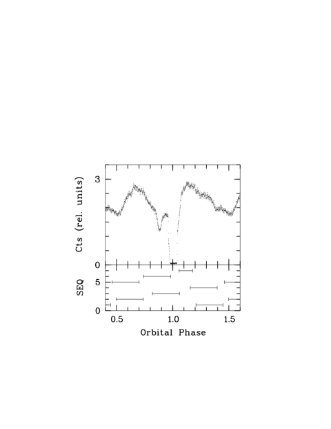
Fig. 1.: (upper panel) Phase-averaged optical B-band lightcurve of HU Aqr for the period August 16-18, 1993. The counts of HU Aqr were reduced to that of a simultaneously observed nearby comparison star. Binsize of the lightcurve is 3.75 sec (2000 phase bins). (lower panel) Phase coverage of the individual trailed spectra of length 30 min (no. 1-6) and 12.5 min (no. 7).

In order to avoid velocity smearing a radial velocity study of an AMHerculis binary requires a phase resolution of $\Delta\phi\simeq 0.05$ (Mukai 1988), hence $\sim$6^m for a binary like HUAqr with period $P_{\rm orb}=125^{m}$. The time overhead between subsequent exposures at the TWIN, on the other hand, is $\sim$5^m due to CCD-readout, data transfer and storage of the large-format images from both arms of the spectrograph, which prevents a dense phase coverage. We resolved the time conflict by trailing the object along the slit while exposing. Individual exposure times were 30^m with a nominal trailing rate of 15 sec/pixel, which, taking into account the size of the seeing disk of $\sim$2pixels, finally yielded a time resolution of $\sim$30 sec or 0.004 phase units. A total of 6 spectra with 1800 s and one with 750 s integration time were obtained yielding full-phase coverage. Wavelength calibration of the flatfielded and bias-subtracted two-dimensional images was performed using Helium-Argon arc spectra taken every hour, a small shift of the arc line pattern on the CCD due to flexure of the spectrograph was accounted for during reduction of the data. Cosmic-ray removal was achieved by median filtering small regions of size $5\times 5$ pixels around suspected cosmics which were identified by Laplace-filtering of the raw images. Sky-subtraction was performed afterwards in the usual manner by fitting polynomials to CCD-columns above and below the region exposed to the target star.

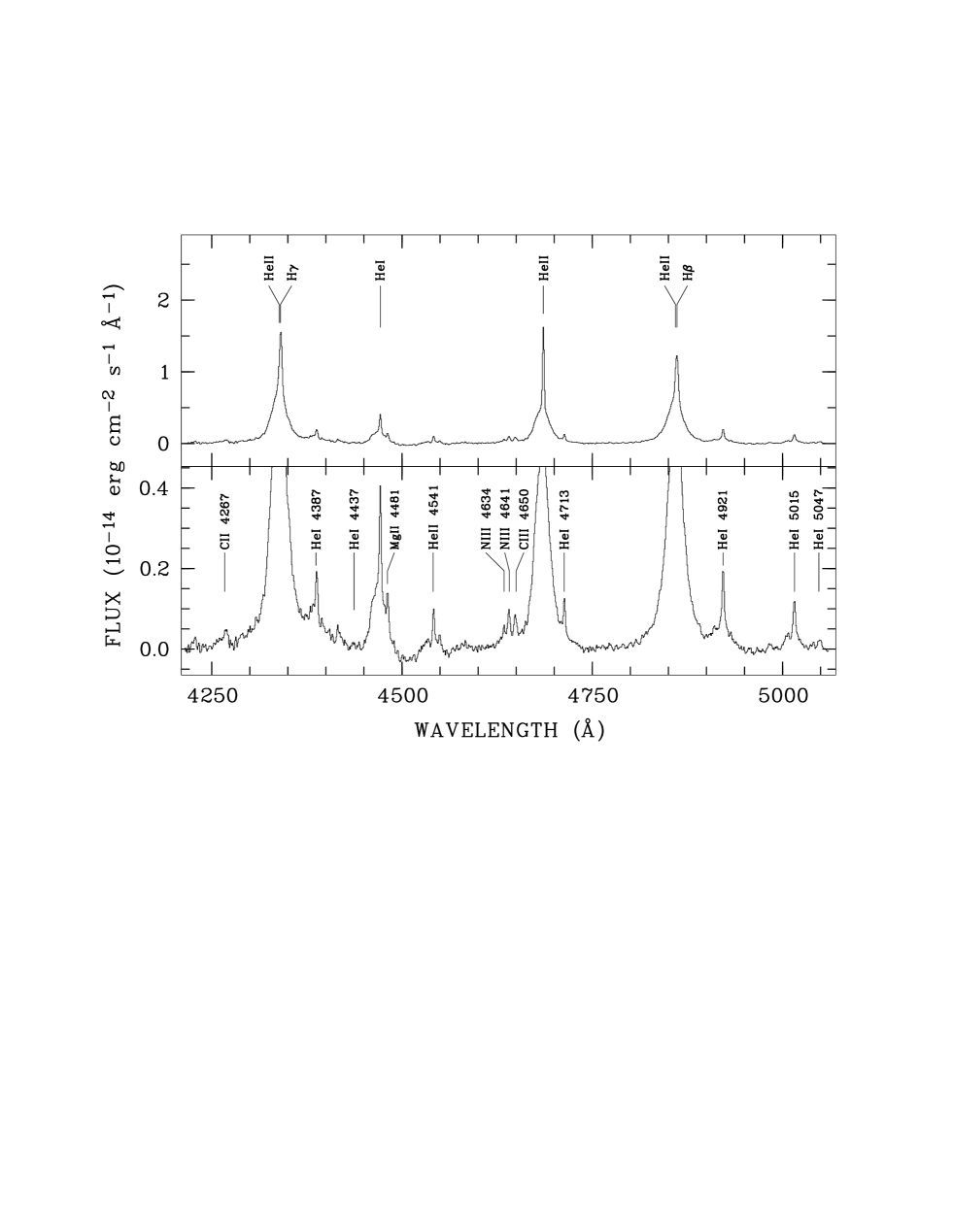
Fig. 2.: Mean-orbital high-resolution spectrum of HUAqr on August 17, 1993, after subtraction of the continuum and after correction to zero velocity (narrow emission line). The same data are shown twice, in the bottom panel on an expanded intensity scale in order to facilitate identification of faint lines

Next, the spatial coordinate of individual pixels along the slit had to be transformed to time or orbital phase. We defined start and end of the exposure as coniciding with those pixels lying most nearly to half intensity between average sky- and (sky+object)-level in an adjacent 10 pixel surrounding. This resulted in a trailed spectrum with 116 or 117 pixels for an 1800 sec exposure, slightly different from the 120 pixels expected from the nominal trailing rate of the telescope. Since the lightcurves extracted from the trailed spectrograms and the simultaneous photometry yielded no systematic offset, we assigned the discrepancy to a slightly incorrect trailing rate of the telescope and estimate the timing accuracy of the spectrum in a single CCD-row to be better than 15 sec.

Simultaneously to our spectroscopy we obtained high-speed photometric data (0.5 sec resolution) using the 2.2m-telescope also located at Calar Alto which was equipped with the MCCP (Barwig et al.1987). The MCCP allows monitoring of the target star, a comparison star and the nearby sky simultaneously in UBVRI colours. In order to correct slit-losses and guiding errors of our trailed spectra, we first flux-calibrated them using observations of the white-dwarf standard star Wolf 1346, folded them through the response of the MCCP B-filter, binned the MCCP-data in 15 sec time bins according to the timing of our trailed spectra and finally multiplied individual rows of the trailed spectra using the ratio of both light curves (photometric, spectroscopic).

Final steps of data reduction included normalization of the spectra by subtracting low-order polynomial fits to the continuum and phase-folding into 100 phase bins using our updated photometric ephemeris of eclipse center

$$T_{\rm ecl}={\rm HJD}244\,8896.543707(27)+E\times 0.086820446(9).$$ (1)

3 Results and analysis

3.1 The lightcurve

In Fig.1 (upper panel) we show the mean light curve in the B-band measured with the MCCP at the 2.2m-telescope. In the lower panel of the diagram the phasing and phase coverage provided by our trailed spectra is displayed. The most remarkable features of the light curve are: a) the deep eclipse of the white dwarf and the accretion spot by the late-type companion star, b) a pronounced pre-eclipse dip centered on phase $\phi_{\rm ecl}$= 0.88, c) a double-humped shape outside eclipse and dip, and d) strong QPO/flaring outside eclipse and dip. A detailed discussion of the light curves will be given elsewhere, in the context of our present analysis the interesting features are the eclipse and the dip.

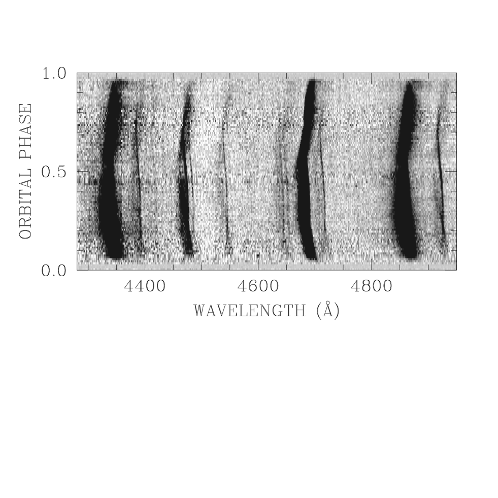
Fig. 3.: Trailed, continuum-subtracted, high-resolution spectrum of HUAqr on August 17, 1993, computed by phase-averaging the individual trailed spectra using 100 phase bins. The dynamic range of this grey-scale image with wavelength running along the abscissa and phase along the ordinate was set appropriately to emphasize weak lines. The behaviour of the strong lines is better visible on the zoomed representations of Fig.4

The eclipse is two-stepped with the first step being very steep ($\sim$3 sec) followed by a more shallow second step with ingress time of about 120 sec. All four steps have different heights. We identify the obscured sources of light with the hot accretion plasma on the white dwarf emitting cyclotron radiation (steep ingress/egress) and the accretion stream (shallow ingress/egress). Both emitters radiate anisotropically which gives the explanation for the different stepsizes at ingress and egress. The eclipse of the white dwarf itself is not clearly resolved in our data. We measured the length of the eclipse as the difference between the maxima in the first derivative of the lightcurve at ingress and egress phase to be 584.6 sec. This value represents the eclipse length of the accretion spot on the white dwarf surface. The spot is nearer to the secondary star than the center of mass of the white dwarf CM_wd. The eclipse of the CM_wd is shorter by a factor $\alpha_{\rm CM}/\alpha_{\rm spot}$ with $\alpha$ being the opening angle of the secondary star as seen from the CM and the spot, respectively. The minimum value of this correction factor is 0.9792 ($\Delta t_{\rm ecl,CM}=572.4$ sec), calculated for the extreme (and therefore unlikely) assumptions of inclination $i=90\hbox{${}^{\circ}$}$ and spot co-latitude $\beta=0\hbox{${}^{\circ}$}$ (spot in the orbital plane).

The Gaussian shaped dip is centered on $\phi_{\rm ecl}$$=0.882\pm 0.003$ (deflection angle $d=42.5\hbox{${}^{\circ}$}\pm 1.1\hbox{${}^{\circ}$}$ with respect to the line joining both stars) and has a FWHM $=0.034\pm 0.001$ phase units. A $\pm 2\sigma$-range around dip center (95% of the absorbed flux) spans a range $d=32\hbox{${}^{\circ}$}-53\hbox{${}^{\circ}$}$. The emission lines are not obscured at dip phase (see Figs.3 and 4), only the cyclotron continuum is absorbed. The dip is therefore naturally explained as obscuration of the accretion spot by the transient accretion stream as in other polars (see Sect.1). Since HUAqr is a system with a high inclination, dip center and width mark exactly the location and extent of the coupling region in the orbital plane.

3.2 The mean orbital spectrum

In Fig.2 we show the mean-orbital, continuum-subtracted, radial-velocity-corrected spectrum of HUAqr. For radial-velocity correction we used the $\sin$-fit to the narrow emission line of He ii $\lambda$4686 (see below). The profiles of the emission lines in Fig.2 therefore show a spiky narrow emission line atop broad line wings. We can identify the emission lines normally found in AM Herculis binaries, as e.g.the Balmer lines H$\beta$ and H$\gamma$, the prominent lines of neutral (He i $\lambda\lambda$4387, 4471, 4713, 4921, 5015) and ionized Helium (He ii $\lambda$4686), but find in addition several features not easily recognized in other systems. We note in particular the partially resolved Ciii/Niii-structure at 4635-4650, Cii $\lambda$4267, a second line of ionized He (Heii $\lambda$4541) with an additional unidentified fainter line in its red wing and Mgii $\lambda$4481 in the red wing of Hei $\lambda$4471.

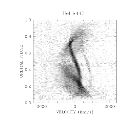
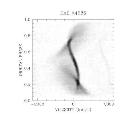
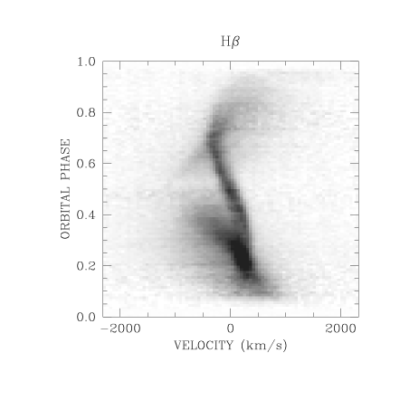
Fig. 4.: Grey-scale representation of trailed, continuum-subtracted, high-resolution spectra of the strong emission lines of HUAqr on August 17, 1993 (zoomed representation of Fig.3). Phase runs along the ordinate from bottom to top, wavelength has been transformed to velocity using the rest wavelengths of the specified lines. The dynamic range for all representations is for all lines approximately between 0 and 80% of maximum intensity.

The Ciii/Niii-complex is resolved into three lines, a single line of Niii ($\lambda 4634.2$) and two blends of Niii ($\lambda\lambda 4640.6,4641.9$) and Ciii ($\lambda\lambda 4647.4,4650.3,4651.5$). The lines of C and N are of comparable strength. According to Williams & Ferguson (1983) the Niii-lines are probably excited by continuum fluorescense. This does not apply to Ciii $\lambda$4650 or to Cii $\lambda$4267 which do not couple directly to the ground states via electric dipole resonance lines. Whereas Cii $\lambda$4267 may be excited by dielectronic recombination no final conclusion was reached by Williams & Ferguson about the probable excitation mechanism of the Ciii-lines, apart from the general statement, that ‘some selective excitation mechanism is operative for this line’. We would like to note simply here that this special excitation mechanism does not require other conditions regarding density, temperature and external radiation field than are required for excitation of the other transitions of the high-ionization species found in the spectrum of HUAqr, since the kinematics and structure of all high-ionization lines seem to be the same.

Three lines of the Heii-Pickering series ($n=4$) lie in our spectral window at $\lambda\lambda$4859.32 ($m=8$), 4541.59 (9), and 4338.67 (10). The line at 4541Å is clearly resolved whereas the other two blend with H$\beta$ and H$\gamma$. The wavelength-difference between the H-Balmer and the Heii-lines is 2.01Å and 1.80Å, respectively, which is at the limit or below our spectral resolution at the specified wavelengths. From our low-resolution spectra we estimate the flux ratio between the non- or weakly-blended lines at 4541.59Å ($m=9$) and 5411.52Å ($m=7$), $F_{5411}/F_{4541}\simeq 1.9$, and interpolate to estimate the contribution of Heii $\lambda$4859 to H$\beta$, which is of the order of 10%, but variable as a function of phase. H$\gamma$ itself is stronger than H$\beta$ and the blending Heii-line ($m=10)$ is weaker than that at H$\beta$, hence we expect a much weaker contamination of H$\gamma$.

The Balmer lines show an inverted Balmer decrement with $I(H\beta)/I(H\gamma)=0.86$. The value for optically thin ‘case B’ recombination is $\sim$2.12 (Pottasch 1984), hence the Balmer lines are significantly optically thick. Although also Heii $\lambda$4686 is not optically thin (see below), the fact that this line is only weakly blended (by Hei $\lambda$4713 and Ciii $\lambda$4650) and that our spectral resolution is highest just at this line makes it the most suitable one in our spectra for detailed investigations, but before doing so we take a general look at the trailed spectrograms.

3.3 Trailed spectra

In Figs.3 and 4 we show the phased-averaged trailed spectra in overview (weak lines emphasized) and for the strong lines H$\beta$, H$\gamma$, He i $\lambda$4471, He ii $\lambda$4686 in detail with a phase resolution of 100 phase bins. In Fig.3 it can be seen that the phase intervals centered on $\phi_{\rm ecl}$= 0.11, 0.46, and 0.78 which were covered only once during our observations have higher noise in the continuum, the effect on the S/N in the strong lines is nevertheless negligible. All emission lines have the same structure and can be subdivided into three emission line components (best visible in He ii $\lambda$4686). Most striking is a narrow emission line (henceforth referred to as NEL), which is most prominent around $\phi_{\rm ecl}$$=0.5$ and which has zero radial velocity at conjunction of the secondary star. This component is naturally explained as being of reprocessed origin from the illuminated hemisphere of the secondary star, seen here in unprecedented clearness. The second component has a more transient nature, it is a relatively narrow line, moving in a zig-zag manner from maximum recessional velocity ($>1000$ km s^-1) around eclipse phase to large negative velocities ($<-1500$ km s^-1) around $\phi_{\rm ecl}$= 0.45. This component is brightest in the phase intervals $\phi_{\rm ecl}$$=0.20-0.25$ and $0.70-0.75$, around those phases where it crosses the NEL. We refer to this component as high-velocity component HVC. The third component is a broad underlying one visible throughout the whole orbital cycle (outside eclipse), with maximum blueshift around $\phi_{\rm ecl}$$\simeq 0.40$ which we refer to as broad base component BBC. The HVC and the BBC must originate in the stream.

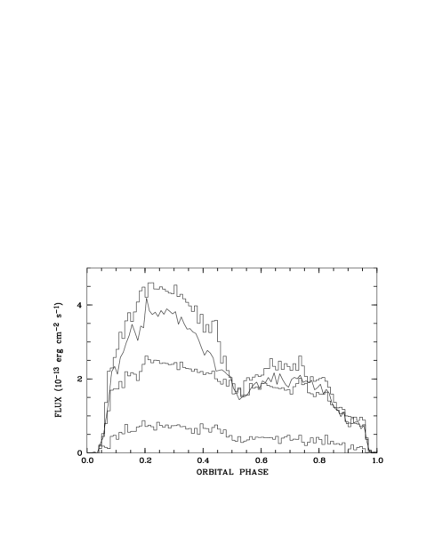
Fig. 5.: Variation of the integrated line flux of the four main emission lines as a function of phase. Shown are from top to bottom the light curves for H$\gamma$ (histogram), H$\beta$ (polygon), He ii $\lambda$4686 , and He i $\lambda$4471.

Although the four main emission lines have the same general appearance differences exist in details. This concerns the width of the NEL, which is broader in the H-Balmer lines than in the He-lines, and the lightcurves of the lines (brightness variation as a function of phase). The width of the NEL of the different lines is addressed in the next section (3.4); the lightcurves are shown in Fig.5 (integrated flux over the wavelength interval used for display in Fig.4). The intensity of the stream components dips to a minimum at phase $\phi_{\rm ecl}$$\simeq 0.53$, and is generally stronger before than after this dip. This asymmetry is generally stronger for the low-ionization lines H$\gamma$, H$\beta$, He i $\lambda$4471 with flux ratios $F(\phi<0.53)/F(\phi>0.53)=2.09,2.14,2.02$, respectively, than for the high-ionization He ii $\lambda$4686-line with the corresponding flux ratio of 1.54.

A likely explanation for the brightness variation of the HVC, which is pronounced only at certain phases, lies in the illumination geometry and significant optical thickness of the stream in the low-ionization lines. The Balmer lines and He i $\lambda$4471 are bright when the stream is seen from its concave, that is its illuminated side (see Fig.14 for a sketch of the geometry). The convex, non-illuminated side of the stream visible after $\phi_{\rm ecl}$$=0.53$ lies in its own shadow and is therefore much fainter than in the less optically thick He ii $\lambda$4686-line.

3.4 The width of the NEL in He- and H-lines

The trailed spectrograms of the Balmer lines (in particular their NELs) look somewhat blurred or diffuse when compared with the He-lines. Here we investigate, if this is caused by the weak blending lines of the Heii-Pickering series mentioned above. The mean width (full width at half maximum FWHM) of the four strongest emission lines (H$\gamma$, He i $\lambda$4471, He ii $\lambda$4686, H$\beta$) in the phase interval $=0.50-0.56$ (NELs intensive, stream components relatively faint) is $(4.19\pm 0.18)$Å, $(2.74\pm 0.15)$Å, $(2.47\pm 0.07)$Å, and $(4.34\pm 0.12)$Å  respectively. The spectral resolution of arc lines at the wavelengths of our lines is 2.33Å, 1.92Å, 1.67Å, and 1.76Å, which yields intrinsic widths of the NEL of 3.48Å, 1.95Å, 1.82Å, and 3.97Å. The He-lines have the same widths within the errors (1.95 vs.1.82Å), whereas the Balmer lines are significantly broader.

We have synthesized blended line profiles of H$\beta$ plus Heii$\lambda 4859$ assuming the same intrinsic line width for both lines of 1.82Å (that of the He ii $\lambda$4686 -line) and a maximum relative intensity of 20% of the He-line. After folding with the instrumental resolution at H$\beta$, the resulting unresolved line had a FWHM of 3.8Å (observed 4.34Å). We conclude that the NELs of the Balmer lines are intrinsically broader than those of the He-lines. Using the same scheme of synthesizing line profiles, we could estimate the width of the H$\beta$-NEL to be $\mathrel{\mathchoice{\vbox{\offinterlineskip\halign{\hfil$\displaystyle#$\hfil\cr>\cr\sim\cr}}}{\vbox{\offinterlineskip\halign{\hfil$\textstyle#$\hfil\cr>\cr\sim\cr}}}{\vbox{\offinterlineskip\halign{\hfil$\scriptstyle#$\hfil\cr>\cr\sim\cr}}}{\vbox{\offinterlineskip\halign{\hfil$\scriptscriptstyle#$\hfil\cr>\cr\sim\cr}}}}3.5$Å. Below we show that the width of the Heii-line is explained by velocity broadening introduced by the range of orbital velocities over the illuminated hemisphere of the secondary star. Hence, each line which originates in that region should have at least this width. If we assume that the observed excess width of H$\beta$ is caused by thermal Doppler broadening, we would need temperatures in excess of $2\times 10^{6}$ K in order to reflect the observations. This temperature, corresponding to coronal temperatures, is unbelievably high for a line originating in a (quasi-)chromosphere. The canonical temperature for the Balmer-line emission region in active M-stars is $10^{4}$ K and the observed line widths at H$\alpha$ are about $\mathrel{\mathchoice{\vbox{\offinterlineskip\halign{\hfil$\displaystyle#$\hfil\cr<\cr\sim\cr}}}{\vbox{\offinterlineskip\halign{\hfil$\textstyle#$\hfil\cr<\cr\sim\cr}}}{\vbox{\offinterlineskip\halign{\hfil$\scriptstyle#$\hfil\cr<\cr\sim\cr}}}{\vbox{\offinterlineskip\halign{\hfil$\scriptscriptstyle#$\hfil\cr<\cr\sim\cr}}}}2$ Å (Giampapa et al.1982, Worden et al.1981). This is also true for irradiated atmospheres of dMe stars although our knowledge of this very complex process is very poor (see e.g.Cram 1982). A more likely explanation seems to be that the observed line width reflects orbital motion of a more extended Balmer line region, perhaps some kind of wind/mass outflow component that co-rotates with the secondary star. An even simpler possibility is ‘saturation broadening’ due to large optical depths in the Balmer lines.

3.5 Gaussian deconvolution of He ii $\lambda$4686

The conventional approach to investigate the emission line structure in polars is fitting of Gaussians. Due to the lack of spectral and temporal resolution often a distinction between a broad and a narrow component is made and only two Gaussians are used but sometimes up to four (Rosen et al.1987). We followed that approach and performed a triple-gaussian fit for the NEL, the HVC and the BBC in an iterative fashion.

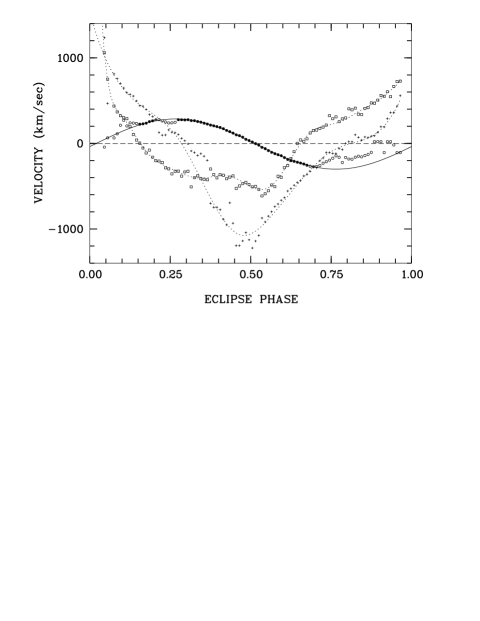
Fig. 6.: Radial velocities of the three subcomponents of He ii $\lambda$4686, determined by fitting Gaussians with fixed widths to the phase-binned spectra shown in Fig.4 (NEL: open and filled circles, HVC: crosses, BBC: squares). The solid line is a $\sin$-fit to the NEL-data shown with filled symbols, the dashed lines are smooth interpolations for the HVC and BBC used as guess-values for subsequent iterations

In a first step we fitted three Gaussians to each of the phase-binned spectra shown in Fig.4 while fixing the widths (FWHM) of the NEL and the HVC at 2.5Åand 4.5Å, respectively. This gave very good estimates for the radial velocities, and good estimates for the line intensities and the FWHM of the BBC. The latter displayed no distinct orbital variation, instead it showed an erratic scatter of 1.5-2 Å around $11.5$ Å. Results for the radial velocities thus obtained are shown in Fig.6. The fits gave unreliable results for the line intensities and for the wavelengths at those phases where two components are crossing each other. This happens at phases $\phi_{\rm ecl}$$\sim$0.23 and $\sim$0.70 between NEL and HVC and at $\phi_{\rm ecl}$$\sim$0.35 between HVC and BBC. In order to provide input guess values for a second iteration, the phase-dependent radial velocities were approximated by smooth curves, a sinusoid for the NEL, spline-curves for the HVC and BBC. The sinusoid and the splines are shown as solid and dashed curves in Fig.6, the sine curve was calculated using only the data points drawn with filled symbols. In a second step we fitted all individual 15 sec spectra in the trailed spectrograms, where these fits were restricted to a small range around the interpolated guess values and the NEL was fixed on the input guess values. Similarly, the phase-binned trailed spectrogram was fitted a second time using these smoothed guess values from the first step but allowing the FWHM to vary freely within certain ranges.

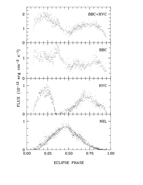
Fig. 7.: Light curves of the three subcomponents of He ii $\lambda$4686, determined by Gaussian fits to individual trailed spectra as described in the text. The uppermost panel represents the summed light from the accretion stream, the lowest that from the secondary star. The solid line in the lowest panel is the result of a model calculation, described in Sect.3.6

The results of these subsequent steps of the fitting procedure, the intensity variations of the three emission line components and the variation of the FWHM of the NEL, are shown in Figs.7 and 10. In Fig.10 we show only those data, for which the NEL could be clearly separated from the HVC. In Fig.7 we also show the summed lightcurve of HVC and BBC representing the light from the stream. The lightcurve of the BBC can be roughly described as a two-stepped function, with constant brightness before and after superior conjunction of the secondary. It is brighter by $\sim$50% during first half of the orbital cycle than during the second half. The hump centered on $\phi_{\rm ecl}$$\simeq 0.35$ is an artefact of the fitting procedure, the excess light there is missing in the HVC-lightcurve, the same may apply to the less pronounced hump at phase 0.82. The lightcurve of the HVC has two pronounced humps separated by $\sim$0.5 in phase with the first hump centered on $\phi_{\rm ecl}$$\simeq$0.22. The sum of both, the HVC and the BBC, shows two smooth humps.

The lightcurve of the NEL finally is single-humped. This component is brightest around superior conjunction of the secondary, but has a remarkable asymmetry with respect to phase 0.5. It is brighter during first part of the orbital cycle, with maximum brightness at $\phi_{\rm ecl}$= 0.46. In some of our fitting experiments, depending on chosen input values and caging of parameters, the brightness of the NEL became even compatible with zero at phases later than 0.75 but it has $\sim$20% of the peak flux at the symmetric phase $\phi_{\rm ecl}$$=0.25$.

The width (FWHM) of the NEL is largest at and slightly after superior conjunction ($\phi_{\rm ecl}$$=0.5$), reaching a maximum value of about 2.45Å. We were prevented from really measuring the width for phases later than $\sim$0.63 due to the decreasing brightness of the NEL and interference with the other line components.

The radial velocity variation of the NEL is in excellent agreement with a $\sin$ curve. The fit assuming a circular orbit for the data points shown with filled symbols in Fig.6, $v(\phi)=v_{\rm sys}+K^{\prime}_{2}\sin(2\pi(\phi-\phi_{0}))$, yields $v_{\rm sys}=-7.8\pm 1.4$ km s^-1, $K^{\prime}_{2}=293.5\pm 1.3$ km s^-1, and $\phi_{0}=0.016\pm 0.001$. There is a small additional systematic uncertainty not larger than $\sim$3 km s^-1for $K^{\prime}_{2}$ dependent on the data points included in the fit. If we correct the systemic velocity to the solar system barycenter, $\Delta v=-3.5$ km s^-1, it becomes $v_{\rm sys}=-11.3\pm 1.4$ km s^-1. We refer to the radial velocity amplitude as $K^{\prime}_{2}$ (instead of $K_{2}$) because it represents the velocity of the center of light of the illuminated hemisphere instead of the center of mass.

Glenn et al.(1994) have presented some 10 high-resolution spectra of H$\alpha$ obtained when the system probably was in a somewhat different state of activity. Probably due to the lack of phase-resolution they discern between a broad and a narrow component only and derive $v_{\rm sys}=83\pm 44$ km s^-1, $K=244\pm 44$ km s^-1, and $\phi_{0}=0.04\pm 0.04$, respectively, for their NEL. The results of both studies are compatible with each other only at the 2$\sigma$-level, hence we cannot completely rule out real changes of the emission line structure. Glenn et al.have described the broad component of H$\alpha$ also with a sinusoid. Given our higher-quality data we cannot use such a simple approach.

Both of our stream components show maximum recessional velocity around eclipse, the full amplitude of the HVC is $\sim$2000 km s^-1, that of the BBC $\sim$1400 km s^-1. Neither the HVC nor the BBC display a radial velocity curve which can be described by a simple mathematical function. An analysis of these components requires a different approach, which is presented below as tomogram analysis. If one, nevertheless, e.g.for comparison with the Glenn et al.analysis, fits a sinusoid to the radial velocity data of the BBC, $v(\phi)=\gamma+K\sin(2\pi(\phi-\phi_{0}))$, one gets $\gamma=3\pm 10$ km s^-1, $K=534\pm 15$ km s^-1, and $\phi_{0}=-0.32\pm 0.01$. Again, these values are compatible with the Glenn et al.analysis at the 1–2$\sigma$ level. One question which is left open here in particular is, whether the two components HVC and BBC originating in the stream really reflect emission from two separate regions, as it appears, or whether instead the emission all along the stream naturally produces skewed profiles simply due to optical depth, projection and curvature of the stream. The conventional approach of deconvolution using Gaussian fits, however, reveals very important information for the interpretation of the tomograms as far as e.g.intensity variation is concerned.

The asymmetrical shape of the lightcurve of the NEL, the non-zero velocity at eclipse and the non-vanishing phase offset $\phi_{0}$ are pronounced and require an interpretation. It appears likely that all three features are related to the same origin, an asymmetric illumination of the secondary star.

3.6 A reprocessing model for the NEL

The skewness of the lightcurve of the NEL is significant. The sole explanation for such an asymmetry is to assume an asymmetric illumination of the secondary star. Similar asymmetries, although mirrored with respect to the axis of symmetry, have been observed by Beuermann & Thomas (1990) in the nova-like UX UMa-system IX Vel and by Hessman (1989) in the dwarf nova IP Peg. The likely mechanism for the asymmetry there is significant irradiation from the hot spot where the accretion stream impacts on the disk. Since this lies on the leading side of the secondary the trailing side is less irradiated and consequently fainter. Such an explanation cannot work in an AM Her binary, since the source of irradiation is bound to the surface of the white dwarf.

A related type of asymmetry has been discovered in NaI absorption lines of AM Her itself by Southwell et al.(1995) and Davey & Smith (1996). These authors detect flux deficits on the trailing side of the secondary in the NaI absorption lines caused by stronger heating of the trailing hemisphere, and explain the necessary shielding of the leading side by absorption in the accretion column near the white dwarf, which points to the leading side in AM Her.

We have synthesized line profiles originating from the illuminated hemisphere of the secondary star using the method as outlined in Horne & Schneider (1989) and Beuermann & Thomas (1990). In this model the Roche lobe surface is covered by a set of discrete surface elements. The flux incident on each surface element is calculated assuming a point source located at the position of the white dwarf. Lightcurves and line profiles are synthesized by summing contributions from all surface elements visible at a given phase. At this stage we allowed for optically thin emission, being proportional to the incident flux, as well as for optically thick emission, where this flux was weighted with the projected surface of the element in concern. No further line broadening mechanism than velocity broadening over the illuminated Roche surface and the instrumental broadening were taken into account. We calculated a series of these profiles as a function of phase and shielding. We took the simple view of describing shielding by a weighting factor for each surface element of the leading side which was constant for the whole hemisphere. We performed such calculations for three values of the mass ratio $Q=M_{\rm wd}/M_{2}=3,4,5$ assuming that the secondary follows the ZAMS mass-radius relationship given by Caillault & Patterson (1990) (in that case the mass of the secondary is $M_{2}=0.146$ M_⊙ and only very weakly dependent on mass ratio) and for $Q=2.5,M_{2}=0.35$ M_⊙, as motivated by our tomogram analysis. The orbital inclination $i$ was chosen according to the $q-i$-relation for the observed length of the eclipse (see Fig.16) as $i=80\hbox{${}^{\circ}$},82\hbox{${}^{\circ}$},85\hbox{${}^{\circ}$},90\hbox{${}^{\circ}$}$, respectively, for $Q=2.5,3,4,$ and 5.

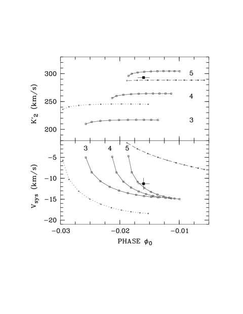
Fig. 8.: Results of model calculations for the NEL: Shown are the relation between radial velocity amplitude, systemic velocity and phase shift obtained from sine fits to synthetic NEL-profiles as a function of mass ratio and shielding of the leading hemisphere of the secondary star. The numbers designate the mass ratio $Q=M_{\rm wd}/M_{2}$. The large open squares connected with solid lines are data computed in the optically thick mode, the small open squares connected with dashed lines are data computed in the optically thin mode (shown only for $Q=5$) and the small circles are optically thin data for $Q=2.5$ with a massive secondary of $M_{2}=0.35$ M_⊙. Shielding increases by 10% between the data points starting with no shielding at right. The large filled squares are observed data.

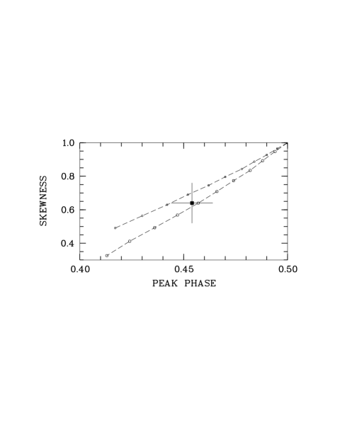
Fig. 9.: Results of model calculations for the NEL: Shown are the relation between skewness ($I(\phi>0.5)/I(\phi<0.5)$) and phase of peak intensity of the NEL-lightcurve for a mass ratio $Q=5$ and varaible shielding of the secondary star. As in Fig.8, shielding grows from right to left in 10%-steps and the larger symbols represent optically thick models. The filled square is the observed value with estimated uncertainties.

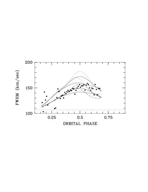
Fig. 10.: Full width at half maximum FWHM of the NEL transformed to velocity at the He ii $\lambda$4686 -line as a function of phase. The filled squares are observed data, the lines are model curves calculated assuming different mass ratios, mass of secondary star, optical thickness and shielding (see text for details). The dotted line at bottom indicates the instrumental resolution.

The synthesized profiles were subsequently analyzed in the same manner as our observed spectra but first their spectral resolution was degraded to a FWHM = 107 km s^-1as observed. Then single Gaussians were fitted to determine the central wavelength. Afterwards sine curves were fitted to the modelled radial velocity data, taking into account only data from those phase intervals which were used also to determine the observed radial velocity curve. The results of this procedure are shown in Figs.8 (parameters of radial velocity curves) and 10 (FWHM vs.phase) together with the observed data. The modelled radial velocity curves are not exact sinusoids, but the deviation is negligible for the phase intervals in concern. Two families of model curves are shown in Fig.10. The upper four curves are calculated for $Q=2.5,M_{2}=0.35$ M_⊙, the lower four for $Q=5,M_{2}=0.146$ M_⊙ (the other models with $M_{2}=0.146$ M_⊙ but smaller $Q$ are undistinguishable from that with $Q=5$). The solid lines are optically thick models, the dashed and dotted lines optically thin. The upper curve of each pair is for no shielding, the lower curve for 60% shielding.

In addition to the line profiles lightcurves for the reprocessed lines as a function of phase were generated. They show a distinct asymmetry in the required manner, which was parametrized using (a) a skewness defined as ratio of fluxes $F(\phi>0.5)/F(\phi<0.5)$ and (b) the phase of maximum intensity. Since these parameters are negligible functions of the mass ratio (they depend only on the adopted shielding), we show in Fig.9 only one set of model data for $Q=5$ and optically thin and thick modes, respectively, together with the parameters derived from the observed lightcurve of the NEL.

The models and data shown in Figs.8 and 9 suggest consistently a mass ratio $Q\simeq 5$, optically thick emission and an effective shielding of the leading side of the secondary star by 60%. Lightcurves for the optically thick and thin models were shown also by Horne & Schneider (1989), where it can be seen that the thin models predict a plateau around $\phi_{\rm ecl}$= 0.5. This happens when always the same numbers of surface elements are visible for a distinct phase interval. Such a plateau is not observed in HU Aqr and we conclude from all the detailed comparisons between our models and the observed data, that the NEL is non-negligibly optically thick.

The fit is not completely satisfactory for the variation of the FWHM. While the low-$Q$, high-$M_{2}$ model predicts too high values for the FWHM for most orbital phases (upper four curves) the model with $Q=5$ predicts somewhat too small values, at least if one takes shielding into account and uses the optically thick models. In addition, shielding moves the phase of maximum FWHM from $\phi_{\rm ecl}$= 0.5 towards smaller values whereas the observed FWHM peaks only at $\phi_{\rm ecl}$$\simeq 0.5-0.55$. We note, however, that the FWHM is the least well determined quantity among all those used here for comparison between observation and models and we do not regard the deviation between observation and simulation as a severe problem.

3.7 Tomogram analysis of the four main emission lines

In this section we investigate the trailed spectrograms shown in Fig.4 using a tomographic inversion technique known as filtered backprojection and described e.g.by Robinson et al.(1993). Making use of such an inversion technique implies that any emission not observed at rest wavelength of a line is regarded as shifted due to the Doppler effect and the backprojection from the observers $(v,\phi)$-space to the original $(v_{x},v_{y})$-plane thus makes use of the whole line profile (instead making use of only e.g.width, intensity or center). The interpretation of such maps is mostly done by comparison with computer-generated schematic drawings of the possible locations of line emission in the binary using as input parameters only the velocites of the two stars of the binary.

The computation of a predicative Doppler-tomogram (or Doppler-map or shortly map) requires a large number of projections (high phase resolution) and a high spectral resolution. Our dataset, in particular the trailed spectrogram of He ii $\lambda$4686, is unique in this respect. The tomograms shown as grey-scale images in Fig.11 and as contourplots in Fig.13 have a velocity sampling of 5 km s^-1 for He ii $\lambda$4686  and 20 km s^-1 for the other lines. Two features in the maps are striking, a bright spot at velocities $v_{x}\simeq 0-30$ km s^-1, $v_{y}\simeq 290$ km s^-1 and a cometary tail linked to it and extending to $v_{x}\mathrel{\mathchoice{\vbox{\offinterlineskip\halign{\hfil$\displaystyle#$\hfil\cr<\cr\sim\cr}}}{\vbox{\offinterlineskip\halign{\hfil$\textstyle#$\hfil\cr<\cr\sim\cr}}}{\vbox{\offinterlineskip\halign{\hfil$\scriptstyle#$\hfil\cr<\cr\sim\cr}}}{\vbox{\offinterlineskip\halign{\hfil$\scriptscriptstyle#$\hfil\cr<\cr\sim\cr}}}}-1000$ km s^-1 at $v_{y}\simeq 0$ km s^-1. A third feature appears as faint smeared blotch in the lower left quadrant of the maps. Since this blotch has a low contrast in Fig.11 only we show in Fig.12 the Doppler map of those emission components of He ii $\lambda$4686  attributed to the accretion stream. It was computed by subtracting the Doppler image of the NEL from that of the complete profile and shows two main features, the cometary tail and the blotch below it.

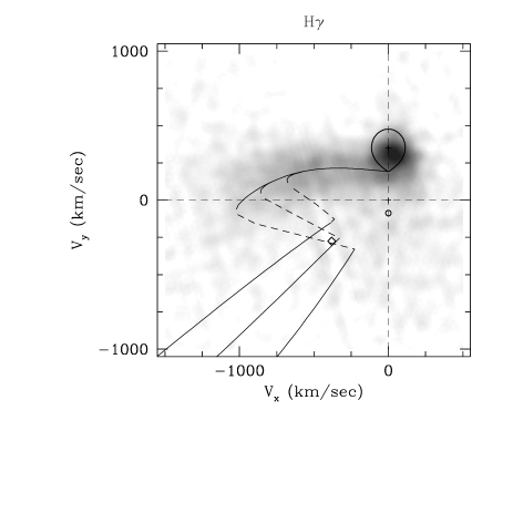
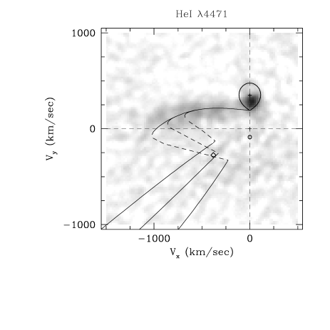
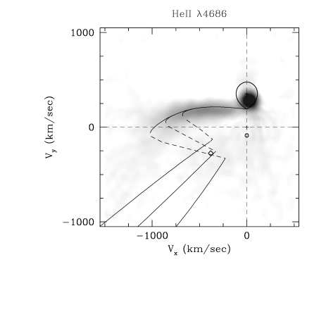
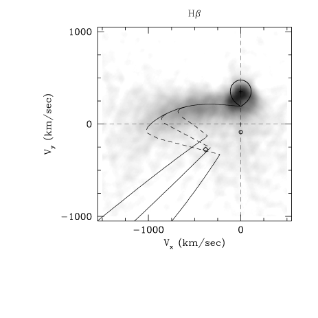
Fig. 11.: Doppler maps of the four main emission lines of HUAqr computed by filtered backprojection of the trailed spectra shown in Fig.4. The velocity resolution for the H$\gamma$-, Hei-, Heii-, and H$\beta$-lines is 161, 129, 107, and 109 km s^-1, respectively, at the origin and 173, 143, 124, 126 km s^-1 at $v=1000$ km s^-1. The overlay shows the shapes of the secondary star and the accretion stream in Doppler coordinates for an assumed mass ratio of $Q=M_{\rm wd}/M_{2}=4$.

Backprojection transforms sine curves to points, the bright spot thus corresponds to the NEL and represents the irradiated secondary star. For the He ii $\lambda$4686-line we compare the position of the spot in the Doppler map with the results of our Gaussian fits. The spot appears at $v_{x}=30$ km s^-1and $v_{y}=283$ km s^-1. The offset of the spot with respect to the symmetry axis $v_{x}=0.0$ reflects the obscuration of the leading (left) side. The ratio of the velocity components corresponds to the measured phase offset $\phi_{\rm 0,sin}$ of the radial velocity curve $\phi_{\rm 0,dop}=(2\pi)^{-1}\arctan(v_{x}/v_{y})=0.017$, in good agreement with $\phi_{\rm 0,sin}=-0.016$. The velocity amplitude $K^{\prime}_{\rm 2,dop}=\sqrt{v_{x}^{2}+v_{y}^{2}}=285$, however, is lower than found from the sine fit to the radial velocity curve $K^{\prime}_{\rm 2,sin}=293.5$ km s^-1. This might be caused by deviations of the true line profiles from Gaussian curves. We see such deviations pronounced in our modelled line profiles in the optically thin approximation and they are present too but less pronounced in the optically thick models (for an illustration see Horne & Schneider, 1989, their Fig.12). We have checked the hypothesis by comparing radial velocities measured (a) by sine fitting radial velocity curves and (b) by 2D-Gaussian fitting in tomograms of our modelled profiles. We indeed find differences of the required type of the order 3–8 km s^-1depending on mass ratio and optically thin/thick approximation. An additional small bias towards lower velocities of the observed peak in the tomogram is likely due to the underlying cometary tail. So we regard both methods to be in agreement. The maps calculated for our synthesized NEL-profiles show that even with our low spectral resolution (with respect to the width of the NEL which is not well sampled) we should have seen a triangle-like structure in the Doppler map sketching the heated ‘nose’ of the secondary star if the emission happens in the optically thin approximation. In the optically thick approximation the modelled tomogram yields only a slightly elongated structure, very similar to what is observed.

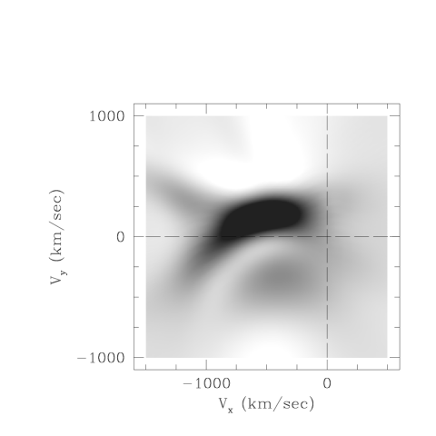
Fig. 12.: Doppler map of the stream components of He ii $\lambda$4686 computed by sutracting the Doppler image of the NEL from the Doppler image of the whole line profile. In order to emphasize the blotch at $(v_{x},v_{y})\simeq(-400,-300)$ km s^-1, we adopted a linear intensity scale between 5% and 60% of the peak intensity.

The Roche lobes shown as overlays in Fig.11 have all the same size thus facilitating a comparison of the four emission lines. The Roche lobes were calculated for a mass ratio of $Q=M_{\rm wd}/M_{2}=4$. According to the larger widths of the NELs of the Balmer lines discussed in Sect.3.4 the corresponding spots are more smeared than those of the Helium lines. In addition, emission is more concentrated towards the equator of the Roche lobe in the Balmer lines. All spots except that in the map of H$\beta$ are bright on the trailing side. The H$\beta$-spot has maximum intensity at $v_{x}\simeq 0.0$ km s^-1 and a longish extension inclined by 135^∘ towards negative $(v_{x},v_{y})$-velocities. The radial velocity amplitudes of the NELs of He i $\lambda$4471, H$\gamma$ and H$\beta$ as measured in the tomograms are $v=284,313,312$ km s^-1, respectively. The value for He i $\lambda$4471  agrees with that of He ii $\lambda$4686, both values for the Balmer lines agree with each other but are significantly higher than those for the Helium lines.

The cometary tail connected to the secondary star in the tomogram is the horizontal accretion stream. It is the Doppler image of the HVC as can be seen directly by mapping only this component singled out using the Gaussian fits. Again this feature appears most brilliant in the map of He ii $\lambda$4686. Its location and curvature in the map are sensitive to the velocities of the stars in the binary and, hence, to the masses and below we will give mass estimates relying on the assumption that the ridge of light exactly reflects the location of the trajectory of the stream (approximated in the usual manner as single particle trajectory, Lubow & Shu 1975, freely falling in the gravitional potential).

Fig. 13.: Contour plots of the Doppler maps for He ii $\lambda$4686 (left) and H$\gamma$ (right) shown in Fig.11 with 11 equidistant contours between 0% and 100% of the peak intensity. The rhombus at $(v_{x},v_{y})\sim(-400,-300)$ km s^-1 indicates the center of BBC emission, the small circle and the cross give the loci of the centers of mass of the white dwarf and the secondary star for the assumed mass ratios of $Q=2.5$ (left diagram) and 5 (right diagram). Shown are the shape of the secondary star, the ballistic trajectory (horizontal stream, upper left quadrant) and the part of the stream which has left the orbital plane (vertical stream, lower left quadrant).

The third component in the Doppler-map, the diffuse blotch in the lower left quadrant, can be identified with the BBC in the trailed spectrogram. This again became evident by mapping the BBC alone which was isolated using the Gaussian fits (the corresponding center of emission of the BBC is marked by a rhombus in Figs.11 and 13). The blotch represents emission from the vertical stream.

We have modelled the location of all components in the tomogram in a manner described e.g.by Marsh & Horne (1988) but included in addition a magnetic drag influencing the trajectory of the stream. The results are shown for two extreme cases of the mass ratio in Fig.13 ($Q=2.5$ and 5, respectively) and for an intermediate value of $Q=4$ in Fig.11. The corresponding picture in positional coordinates is shown in Fig.14. In Fig.15 we show the geometry of the stream as seen by a hypothetic observer at the white dwarf.

The shape of the secondary star projected onto the orbital plane is the same in position and Doppler coordinates, though rotated by 90^∘ in the Doppler coordinates because the orbital velocity vectors are perpendicular to the position vector. Our stream starts at the inner Lagrangian point $L_{1}$ with no initial width. The stream then follows a single particle trajectory (Lubow & Shu 1975) in the Roche-potential down to the interaction region between magnetosphere and accretion stream. The location and size of this stagnation region is determined from the phase and the phase width of the absorption dip (Fig.1). In Figs.13 to 15 we show three trajectories with turn-off points adjusted to reflect the center and width of the stream (distance to center is $\pm 2\sigma$ of Gaussian fitted dip). There the stream leaves the orbital plane as it couples onto field lines. We assumed no dissipation to occur in the interaction region. The abrupt re-orientation of the stream happens in a small spatial region, but produces a large jump in velocity from $\sim$(-1100,0) to $\sim$(-400,-300) in $(v_{x},v_{y})$-space. The stream then follows the field lines of an assumed dipolar field. The field axis was fixed at colatitude $\beta=25\hbox{${}^{\circ}$}$ measured with respect to the rotation axis and azimuth $\Psi=40\hbox{${}^{\circ}$}$ with respect to the line joining both stars. The former value derives from the observed motion of cyclotron lines in low-resolution spectra (Schwope et al.1996, in preparation), the latter one from the phase of the optical/X-ray bright phase center.

We have chosen a model with $Q=4$ ($K_{1}=87$ km s^-1, $K_{2}=350$ km s^-1) for the overlay in Fig.11 which gives a fairly good representation of the four lines and their subcomponents regarded there. We note, however, that the HVC-emission of the He ii $\lambda$4686-, He i $\lambda$4471-, and H$\beta$-lines is concentrated below the line defined by the model, whereas that of the H$\gamma$-line is concentrated above the model line. We find excellent agreement between the HVC-ridge of He ii $\lambda$4686 and the trajectory for a mass ratio of $Q=2.5$ ($K_{1}=147$ km s^-1, $K_{2}=367$ km s^-1) and good agreement for H$\gamma$ using a mass ratio of $Q=5$ ($K_{1}=77$ km s^-1, $K_{2}=384$ km s^-1) (Fig.13).

We see in the tomogram that significant broadening takes place all along the horizontal stream, which is not reflected by our model. This is due to the simplicity of the model which does not take into account any potential broadening mechanism as e.g.the finite width of the stream and its optical thickness.

Fig. 14.: Scheme of the accretion geometry in HUAqr projected onto the orbital plane for an assumed mass ratio $Q=5$. Shown are the loci of the center of mass (cross), the white dwarf (circle) and the secondary star (cross at right) as well as the Roche-lobes of both stars. Matter leaves the secondary star at the $L_{1}-$point and follows a ballistic trajectory. Three field lines connecting the stagnation region and the white dwarf are shown, the region in between is densily dotted. One additional field line (dashed line) connects the inner Lagrangian point with the white dwarf. The region between this line and the dense vertical stream, where the accretion curtain is located, is dotted lightly.

It is somewhat surprising that we cannot detect emission from the stream at really high velocities ($>700$ km s^-1) close to the white dwarf ($v_{\rm ff}\simeq 4000$ km s^-1). This may reflect the effects of a high degree of ionization and small radiating surface of the stream at high velocities. Possible effects which in addition may contribute to the low velocities in the BBC (and its Doppler image, the blotch) are (a) a slightly incorrect continuum subtraction thus removing faint emission at high velocities, and (b) emission not only from the accretion stream but also from the accretion curtain, hence from matter leaving the plane all along the horizontal stream. This matter is thought to be responsible for shadowing of the leading side of the secondary star and its re-emission has not been regarded so far. The turn-off points of such trajectories lie closer to the $L_{1}$ and the jumps from the HVC- to the BBC-region in the map are smaller thus closing the expected gap. One sees also that the observed large width of the BBC is introduced naturally by the models due to the simple fact that coupling happens along the trajectory over a significant distance and the jumps from the HVC- to the BBC-region adjust correspondingly. In principle, so-called ‘gamma-smearing’ may contribute to the observed width of the BBC in the Doppler map (Diaz & Steiner 1994). Gas with velocity perpendicular to the orbital plane $v_{z}$ produces a shift $\gamma=v_{z}\cos i$. The effect of this is to blur the corresponding feature in the Doppler map over a ring of radius $\gamma$ centered at its usual position. If we assume $v_{z}=1000$ km s^-1and $i$ in the range 81^∘–85^∘, we get a smearing amplitude of $156-87$ km s^-1, which is of the order of or below the resolution of our map. Hence, our map of HUAqr is essentially blind to the vertical motions.

Fig. 15.: Scheme of the accretion geometry in HUAqr as seen by a hypothetical observer located at the center of the white dwarf. Matter leaves the secondary star at the $L_{1}-$point and follows a ballistic trajectory, hence it is deflected under the influence of Coriolis forces to the left. The stream leaves the orbital plane and couples onto field lines at an azimuth of 43^∘, where the absorption dip occurs. Three field lines connecting the stagnation region and the white dwarf are shown indicating the width of the absorption dip (dark dotted region). One additional trajectory (dashed line) is shown leaving the plane at the $L_{1}-$point. The region between this line and the dense vertical stream is less dense dotted (accretion curtain).

In Figs.14 and 15 the distribution of matter in the system is shown. The dark shaded region in both figures are the horizontal and vertical streams, while the dotted region gives a schematic of the accretion curtain necessary for shielding the leading hemisphere. This curtain is constrained by a trajectory which couples to the magnetic field at the $L_{1}$-point. This gives not the required 60% derived above obscuration indicating that the view taken here is still too simplistic. Additional obscuration will be provided by nature by the finite width of the stream at the $L_{1}$ which is of the order of 10% of the secondary star’s radius.

We can use our stream models to obtain estimates for physical parameters of the stagnation region. The extent of this region in the orbital plane (length along the trajectory) is $l\simeq 6\times 10^{9}$ cm and along which the undisturbed dipole field strength varies between 3 and 9 kG. The polar field strength was set to $B=38$ MG which yields a field strength in the accretion spot of about 36-37 MG as required by the identification of cyclotron harmonics (Schwope et al.1993, Glenn et al.1994). Our code assumes a constant cross section along the trajectory, $\rho v=\dot{m}=\rm{constant}$. Coupling at different loci along the trajectory is possible by a variation of the density $\rho$, thus varying the ram pressure $p_{\rm ram}\propto\rho v^{2}$ of the stream. Under these assumptions we found that the ratio of the ram and magnetic pressure varies by a factor of 6–7 along the trajectory in the stagnation region. The size of the stagnation region is transferred down to the white dwarf surface via dipole field lines where it occupies a region with full opening angle of about 5^∘–6^∘corresponding to a linear dimension of $l\simeq 7\times 10^{7}$ cm for a white dwarf with radius $R_{\rm wd}=7\times 10^{8}$ cm.

The tomogram together with the schemes of the accretion geometry also yields hints for an understanding of the lightcurves of the HVC and the BBC (Fig.7). Both components are brighter during first half of the orbital cycle, when we view the magnetic curtain’s concave illuminated side. The HVC is bright and easily to recognize in the trailed spectrogram around quadrature phases. The observed spectra at these phases correspond to projections of the map parallel to the $v_{x}-$axis, hence along the cometary tail, producing a sharp feature in a spectrogram. The observed spectra at conjunction phases, on the other hand, correspond to projections along the $v_{y}-$axis. At these phases emission from the horizontal stream is smeared over an interval of $\sim$1000 km s^-1 which produces only very broad spectral features. Hence, at theses phases the HVC apparently vanishes and we obtain the minima in the lightcurve of the HVC.

4 Discussion and conclusions

We have found two distinct features in the trailed spectrograms of the four main emission lines in the blue spectral regime of HUAqr, in particular the line of ionized Helium He ii $\lambda$4686, which are potentially useful for a determination of the stellar masses. These are the amplitude of the radial velocity curve of the narrow emission line NEL and the location and curvature of the horizontal stream in the tomogram, the Doppler image of the HVC. An additional constraint on the mass ratio is set by the observed eclipse length. All these constraints are shown in a $(Q,i)-$plane in Fig.16 with $Q$ being the mass ratio and $i$ the orbital inclination. The eclipse length is dependent on the size of the secondary star’s Roche lobe and the inclination, hence relation (1) in the diagram is purely geometrical (it is of course implicitly assumed that the secondary fills exactly its Roche lobe) (Chanan et al.1976). The solid line is valid for the measured eclipse length, the nearby dashed line is valid for the maximum correction which accounts for the offset of the accretion spot from the white dwarfs center, see above. Relation (2) in the diagram for the NEL makes use of a factor which relates the center of light of the illuminated hemisphere to the center of mass. This factor is dependent on $Q$ and shown in Horne & Schneider (1989) for the optically thin and in Schwope et al.(1993) for the optically thick models. The differences between both modes are negligible as far as this factor is concerned. The computation of the curves (2) in the $(Q,i)-$plane makes use further of the Roche geometry (approximation of the spherical equivalent Roche-radius as a function of $Q$ given by Eggleton (1983)) and Kepler’s third law. We have assumed that the secondary is a main sequence star and can be described by a ZAMS mass-radius relation for late-type stars. With $M_{2}=0.146$ M_⊙, the empirical relation by Caillault & Patterson (1990) predicts the least compact secondary for HUAqr, the other extreme with $M_{2}=0.206$ M_⊙ is due to the relation by VandenBerg et al.(1983) (solid and dashed lines in Fig.16). Relation (3) finally is the result of a fit-per-eye to the location and curvature of the horizontal stream in the tomogram which relies on the assumption that the center of light along the ridge of He ii $\lambda$4686  marks the single-particle trajectory. This results in the smallest estimates of $Q$ with $Q\simeq 2.5$.

Fig. 16.: Mass determination of HUAqr using the observed length of the eclipse (1), the radial velocity amplitude of the illuminated hemisphere of the secondary star with different mass-radius relations (2), and the curvature of the ballistic stream in the Doppler map (3).

It is clear from Fig.16 (as well as from several previous Figures) that no unique solution exists presently in the framework of the models presented here. Relations (1) and (2) suggest high values of the mass ratio and the inclination with $Q\simeq 4.5-5.5,i>85\hbox{${}^{\circ}$}$ for the Helium lines and $Q=5-5.5,i>87\hbox{${}^{\circ}$}$ for the Balmer lines (the latter are not shown in Fig.16). The curvature of the stream of He ii $\lambda$4686, He i $\lambda$4471 and H$\beta$ on the other hand suggests, that the mass ratio might be as low as $Q=2.5$ and that the inclination correspondingly might be as low as $i\simeq 80\hbox{${}^{\circ}$}$. Both estimates of the mass ratio seem to exclude each other presently and it appears likely that neither the NEL (in combination with $K_{2}$-correction and ZAMS-approximation) nor the HVC (fitted by a single-particle trajectory) can be used straightly to give an accurate mass estimate.

The disagreement between both approaches becomes smaller if one assumes that NEL emission is more concentrated towards the center of mass of the secondary than we have assumed. An absorbing cloud of matter in the $L_{1}$-region which would suppress emission from the ‘nose’ of the secondary could e.g.provide the necessary bias of the effective radial velocity amplitude towards higher values (and could also lower the width of the line profiles, Fig.10). The expected re-emission might be responsible for the longish extension of the bright spot near the $L_{1}$-point in the tomogram of H$\beta$. That such bias exists appears likely from the observed higher NEL-velocity of the Hydrogen Balmer lines with respect to the Helium lines. The ‘nose’ is more effectively shielded in the more optically thick Hydrogen lines.

The best way to solve the conflict and to calibrate the M/R-relation of the secondary star would be to measure the radial velocity of the secondary star independently using e.g.photospheric absorption lines. This will help to sort out which feature (NEL, HVC) of which line may serve as the estimator of the mass ratio. It requires HUAqr to be observed in a low state of accretion. Such a measurement is highly demanded in order to calibrate either of the methods used here for mass determination. Another hint to the likely mass of the stars and the mass ratio could be derived from ingress/egress length into/from eclipse of the white dwarf itself, rather than ingress/egress of the accretion spot on it.

Our model with $Q=2.5$ implies that the secondary star in HUAqr must be as massive as 0.35 M_⊙. It would be much more compact than a ZAMS-star and in consequence much more luminous. This would imply that the distance estimates given by Glenn et al.(1994) and Schwope et al.(1993) are lower limits only.

We have presented high-resolution spectral observations of the eclipsing AM Herculis star HUAqr obtained when the system was in a high state of accretion. We have identified three emission line components in our trailed spectra of He ii $\lambda$4686, He i $\lambda$4471, and the H-Balmer lines. These could be uniquely identified as originating on the illuminated hemisphere of the secondary star (the narrow emission line NEL), the stream in the orbital plane (the high-velocity component HVC) following a ballistic trajectory, and the stream coupled onto field lines out of the orbital plane (the broad-base component BBC). We have uniquely identified the horizontal stream in this AM Her-binary by means of Doppler tomography and could trace it from the $L_{1}$-point down to the stagnation region. On the assumption that the NEL of He ii $\lambda$4686 is formed on the surface of the Roche-lobe of the companion star we have determined its mass. This estimate is in disagreement with an estimate derived from the tomogram. We propose that Doppler tomography of the ballistic stream can be used as a new tool for the mass determination of accreting binaries provided we can calibrate this method using an independent mass determination.

• We thank M.Giampapa for helpful comments concerning chromospheric emission from late-type stars and H.Ritter for useful hints concerning their mass-radius relation. We thank an anonymous referee for helpful comments. This work was supported in part by the Deutsche Forschungsgemeinschaft under grant Schw 536/4-1 and the BMFT under grant 50 OR 9403 5.

References

- Barwig H., Schoembs R., Buckenmayer C., 1987, A&A 175, 327
- Beuermann K., Thomas H.-C., 1990, A&A 230, 326
- Beuermann K., Thomas H.-C., Schwope A.D., Giommi P., Tagliaferri G., 1990, A&A 238, 187
- Caillault J.–P., Patterson J., 1990, AJ 100, 825
- Chanan G.A., Middleditch J., Nelson J.E., 1976, ApJ 208, 512
- Cram L.E., 1982, ApJ 253, 768
- Davey S.C., Smith R.C., 1996, MNRAS, in press
- Diaz M.P., Steiner J.E., 1994, A&A 283, 508
- Eggleton P.P., 1983, ApJ 268, 368
- Giampapa M.S., Worden S.P., Linsky J.L., 1982, ApJ 258, 740
- Glenn J., Howell S.B., Schmidt G.D., Liebert J., Grauer A.D., Wegner R.M., 1994, ApJ 424, 967
- Hakala P.J., Watson M.G., Vilhu O., Hassall B.J.M., Kellett B.J., Mason K.O., Piirola V., 1993, MNRAS 263, 61
- Hessman F.H., 1989, AJ 98, 675
- Horne K., Schneider D.Q., 1989, ApJ 343, 888
- Marsh T.R., Horne K., 1988, MNRAS 235 269
- McCarthy P., Clarke J.T., Bowyer S., 1986, ApJ 311, 873
- Mukai K., 1988, MNRAS 232, 175
- Liebert J., Stockman H.S., 1985, in: CVs and LMXBs, eds.D.Q.Lamb and J.Patterson, p.151
- Lubow S.H., Shu F.H., 1975, ApJ 198, 383
- Pottasch S.R., 1984, Planetary Nebulae, Reidel, Dordrecht
- Robinson E.L., Marsh T.R., Smak J.I., 1993, In: Accretion Disks in Compact Stellar Systems, World Sci.Publ.
- Rosen S., Mason K.O., Cordova F.A., 1987, MNRAS 224, 987
- Schmidt G.D., Liebert J., Stockman H.S., Holberg J., 1993, Ann.Isr.Phys.Soc.10, 13
- Schwope A.D., 1991, PhD thesis, TU Berlin
- Schwope A.D., Thomas H.-C., Beuermann K., 1993b, A&A 271, L25
- Schwope A.D., Beuermann K., Thomas H.-C., Reinsch K., 1993a, A&A 267, 103
- Schwope A.D., Thomas H.-C., Beuermann K., Naundorf C.E., 1991, A&A 244, 373
- Schwope A.D., Schwarz R., Mantel K.-H., Horne K., Beuermann K., 1995, ASP Conf.Ser.85, D.Buckley and B.Warner (eds.), p.166
- Shafter A.W., Reinsch K., Beuermann K., Misselt K.A., Buckley D.A.H., Burwitz V., Schwope A.D., 1995, ApJ 443, 319
- Southwell K.A., Still M.D., Smith R.C., Martin J.S., 1995, A&A 302, 90
- VandenBerg D.A., Hartwick F.D.A., Dawson P., Alexander D.R., 1983, ApJ 266, 747
- Watson M., 1995, ASP Conf.Ser.85, D.Buckley and B.Warner (eds.), p.179
- Williams R.E., Ferguson D.H., 1983, In: Cataclysmic Variables and Related Objects, eds.M.Livio and G.Shaviv, Reidel, Dordrecht, p.97
- Worden S.P., Schneeberger T.J., Giampapa M.S., 1981, ApJS 46, 159