A. Kogut

Hughes STX Corporation
Laboratory for Astronomy and Solar Physics
Code 685, NASA/GSFC, Greenbelt, MD 20771

G. Hinshaw

Laboratory for Astronomy and Solar Physics
Code 685, NASA/GSFC, Greenbelt, MD 20771

A.J. Banday

Max Planck Institut für Astrophysik
85740 Garching Bei München, Germany

Accepted for publication in Physical Review D15

ABSTRACT

Small departures from a homogeneous isotropic spacetime create observable features in the large-scale anisotropy of the cosmic microwave background. We cross-correlate the maps of the cosmic microwave background anisotropy from the Cosmic Background Explorer (COBE) Differential Microwave Radiometers (DMR) 4-year data set with template maps from Bianchi VII_h cosmological models to limit global rotation or shear in the early universe. On the largest scales, spacetime is well described by the Friedmann-Robertson-Walker metric, with departures from isotropy about each spatial point limited to shear $\sigma/H_{0}<10^{-9}$ and rotation $\omega/H_{0}<6\times 10^{-8}$ for $0.1{{}_{<}\atop{}^{=}}\Omega_{0}{{}_{<}\atop{}^{=}}1$.

PACS numbers: 98.80.ES, 98.70.Vc

I INTRODUCTION

One of the goals of cosmology is to understand the large scale structure of the universe. Gravitational instability models hold that large-scale structure forms as the result of gravitational amplification of initially small perturbations in the primordial density distribution. The initial “seeds” may result from quantum fluctuations in a scalar field (inflation) or causal ordering following a phase transition with broken symmetry (topological defects), but in all models the evolution occurs in a “background” cosmology described by the Friedmann-Robertson-Walker (FRW) metric.

The anisotropy of the cosmic microwave background (CMB) provides an observational test of the the assumption that on large scales spacetime asymptotically approaches the FRW metric. The detection of fluctuations in the CMB provides support for a nearly homogeneous spacetime, limiting density perturbations in the early universe to the level $\delta\rho/\rho\approx 10^{-5}$. The CMB anisotropy also provides a direct test of the assumption of isotropy about each spatial point. Small deviations from the FRW metric lead to observable signatures in the CMB. Open or flat models with global rotation or shear will exhibit a spiral pattern of temperature anisotropy resulting from the handedness of the geodesics propagating through an anisotropic spacetime. Further geodesic focusing creates “hot spots” in open models (density $\Omega_{0}<1$), while closed models exhibit a pure quadrupole pattern.

Several authors have used the CMB to limit rotation $\omega$ and shear $\sigma$ in the universe [1, 2, 3, 4]. Prior to the detection of CMB anisotropy, Collins & Hawking and Barrow, Juskiewicz, & Sonoda used upper limits on the CMB quadrupole amplitude to limit $\omega/H_{0}<10^{-5}$ for flat or moderately open ($\Omega_{0}\approx 0.3$) models. Smoot used the quadrupole detection from the first-year COBE DMR sky maps to limit $\omega/H_{0}<10^{-6}$. Recently, Bunn, Ferreira, & Silk fitted the full spiral pattern from models with global rotation to the 4-year DMR data and derived limits $\omega/H_{0}<3\times 10^{-7}$.

The DMR anisotropy data are dominated by a power-law spectrum of fluctuations which are ill-described by the pattern of angular anisotropy predicted for models with global rotation or shear. Limits to rotation or shear based on full-sky “template” maps must account for the presence of this power-law component. Bunn, Ferreira, & Silk [4] use a least-squares fit including only instrument noise, and then account for chance alignment of the spiral template map with features in the power-law component using Monte Carlo simulations. In this paper, we present an independent analysis using a formalism which expressly includes the dominant power-law component in the fitting process, and derive upper limits $\omega/H_{0}<6\times 10^{-8}$ for $0.1{{}_{<}\atop{}^{=}}\Omega_{0}{{}_{<}\atop{}^{=}}1$.

II GEOMETRY

The FRW geometry is a special case of more general solutions to the Einstein field equations. Relaxing the requirement of isotropy about each point leads to more complicated solutions which contain the FRW metric as a special case. The Bianchi models VII_h, VII₀, and IX are the most general solutions for a homogeneous but anisotropic universe which contain the open, flat, or closed FRW metric as a special case. The metric is defined as

$$g_{\mu\nu}=-{\rm n}_{\mu}{\rm n}_{n}u~{}+~{}g_{\rm AB}{\rm E}^{\rm A}_{\mu}{\rm E}^{\rm B}_{\nu}$$

where n${}_{\mu}=-t_{;\mu}$ is the normal to the spacelike surfaces of homogeneity, $g_{\rm AB}$ is a $3\times 3$ matrix depending only on t, and E${}^{\rm A}_{\mu}$ are the three invariant covector fields in the surfaces of homogeneity such that

$${\rm E}^{\rm A}_{\mu;\nu}-{\rm E}^{\rm A}_{\nu;\mu}={\rm C}^{\rm A}_{\rm BC}{\rm E}^{\rm B}_{\mu}{\rm E}^{\rm C}_{\nu}$$

where C${}^{\rm A}_{\rm BC}$ are the structure constants (see, e.g., Ellis & MacCallum [5]). The matrix $g_{\rm AB}$ can be expanded into a part representing the expansion and a trace-free part representing the anisotropy,

$$g_{\rm AB}={\rm e}^{2a}[{\rm e}^{2\beta}]_{\rm AB}.$$

The metric anisotropy in these models is characterized by the vorticity $\omega$ and the shear $\sigma$ (differential expansion in orthogonal directions),

$$\omega^{\mu}=\frac{1}{2}\eta^{\mu nu\lambda\rho}{\rm u}_{\nu}{\rm u}_{\lambda;\rho}$$

$$\sigma_{\rm ij}=\frac{1}{2}\left[(\exp({\beta}))^{\bullet}(\exp({-\beta}))+(\exp({-\beta}))(\exp({\beta}))^{\bullet}\right]_{\rm ij}$$

where u is the four-velocity, $\eta^{\mu\nu\lambda\rho}$ is an anti symmetric tensor and the dot represents a time derivative. The FRW metric is recovered in the limit $\omega/H_{0}\rightarrow 0$ and $\sigma/H_{0}\rightarrow 0$ where $H_{0}$ is the Hubble constant.

Photons propagate along geodesics from the surface of last scattering to the observer; for small metric anisotropies the CMB anisotropy is

$$\frac{\Delta T}{T}=({\rm p}^{\rm i}{\rm u}^{\rm i})_{\rm R}-({\rm p}^{\rm i}{\rm u}^{\rm i})_{\rm E}-\int_{\rm R}^{\rm E}{\rm p}^{\rm j}{\rm p}^{\rm k}\sigma_{\rm jk}dt$$

where pⁱ are the direction cosines of the null geodesic and the subscripts E and R refer to emission and reception, respectively. The first two terms are the Doppler anisotropy from the motion of the receiver and the surface of last scattering, while the last term represents the geodesics integrated over the anisotropic metric. Various authors have solved the geodesic equations for the observed pattern of CMB anisotropy [1, 2, 6]. In this paper, we specialize to Bianchi VII_h model ($C^{2}_{31}=C^{3}_{21}=1$ and $C^{2}_{21}=C^{3}_{31}=\sqrt{h}$), which contains the Bianchi I, V, and VII₀ models in the appropriate limit. Two effects are important. The intrinsic handedness of the tensor $\sigma_{\rm ij}$ causes the geodesics to spiral in open or flat models. The resulting temperature pattern is given by

$$\frac{\Delta T}{T}~{}=~{}\left(\frac{\sigma}{H}\right)_{0}[~{}A(\theta_{\rm R})\sin\phi_{\rm R}~{}+~{}B(\theta_{\rm R})\cos\phi_{\rm R}]$$ (1)

(Barrow, Juskiewicz, and Sonoda [2]), where ($\theta_{\rm R},\phi_{\rm R}$) specify the photon direction,

$$A(\theta_{\rm R}) = C_{1}[\sin\theta_{\rm R}-C_{2}(\cos\psi_{E}+3\sqrt{h}\sin\psi_{E})]$$ (2)

$$+~{}C_{3}\int^{\tau_{\rm R}}_{\tau_{E}}\frac{s(1-s^{2})\sin\psi d\tau}{(1+s^{2})^{2}{\rm sinh}^{4}(\sqrt{h}~{}\tau/2)},$$

$$B(\theta_{\rm R}) = C_{1}[3\sqrt{h}\sin\theta_{\rm R}-C_{2}(\sin\psi_{E}+3\sqrt{h}\cos\psi_{E})]$$ (3)

$$-~{}C_{3}\int^{\tau_{\rm R}}_{\tau_{E}}\frac{s(1-s^{2})\cos\psi d\tau}{(1+s^{2})^{2}{\rm sinh}^{4}(\sqrt{h}~{}\tau/2)},$$

$$s=\tan\left(\frac{\theta_{\rm R}}{2}\right)\exp[-\sqrt{h}(\tau-\tau_{\rm R})],$$ (4)

$$\psi=(\tau-\tau_{\rm R})-\frac{1}{\sqrt{h}}\ln\left\{\sin^{2}\left(\frac{\theta_{\rm R}}{2}\right)+\exp[2\sqrt{h}(\tau-\tau_{\rm R})]\cos^{2}\left(\frac{\theta_{\rm R}}{2}\right)\right\},$$ (5)

and $dt={\rm e}^{a}d\tau$. The constants $C_{1}$, $C_{2}$, and $C_{3}$ are defined as

$$C_{1}=\frac{1}{3\Omega_{0}x}$$

$$C_{2}=\frac{2s_{E}(1+z_{E})}{1+s^{2}_{E}}$$

$$C_{3}=\frac{4\sqrt{h}(1-\Omega_{0})^{3/2}}{\Omega_{0}^{2}},$$ (6)

where $z$ is redshift and the parameter

$$x=\sqrt{\frac{h}{1-\Omega_{0}}}$$

determines the scale over which the principal axes of shear and rotation change orientation. We obtain the Bianchi VII₀ model in the limit $\Omega\rightarrow 1,h\rightarrow 0$ with $x$ finite; we obtain the Bianchi I model as $x\rightarrow\infty$ and the Bianchi V model as $h\rightarrow\infty$.

The ratio $\sigma/H_{0}$ determines the amplitude of the anisotropy, while the parameter $x$ determines the pitch angle of the spiral. A significant amount of the resulting CMB anisotropy is present at high-order moments than the quadrupole. A second effect is geodesic focusing, present only in open models. The component of the geodesics along the symmetry axis transforms in these models as

$$\tan\left(\frac{\theta}{2}\right)=\tan\left(\frac{\theta_{\rm R}}{2}~{}\exp(\tau_{\rm R}-\tau)\right).$$

Since

$$\sinh\left(\frac{\tau}{2}\right)~{}\approx~{}\frac{\Omega^{-1}-1}{1+z},$$

the spiral anisotropy discussed above is focused into a single hot “navel” $\approx~{}\Omega_{0}$ radians in scale oriented along the symmetry axis of the metric. Figure 1 shows a polar projection of the anisotropy for $\Omega_{0}=0.3$ and $x=0.5$.

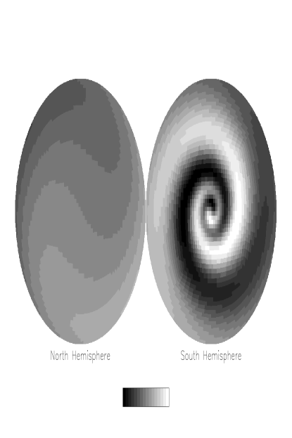
Figure 1: Anisotropy template map (arbitrary units) for a Bianchi VII_h model with $\Omega_{0}=0.3$ and $x=0.5$. Note the differences between the hemispheres from geodesic focusing.

III ANALYSIS

The DMR 4-year sky maps are well described by a superposition of instrument noise and nearly scale-invariant CMB anisotropy, in the sense that the observed sky falls near the median of the distribution of simulated skies which include only these two components [7]. We test for the presence of a third component of unknown amplitude whose spatial distribution is described by a Bianchi VII_h model,

$$\Delta T^{\rm DMR}=\Delta T^{CMB}~{}+~{}\alpha\Delta X~{}+~{}n,$$

where $\Delta T^{\rm CMB}$ is the thermodynamic temperature of the scale-invariant CMB anisotropy, $\Delta X$ is a “template” map of a specific Bianchi model, and $n$ is the DMR instrument noise. We do not analyze the closed Bianchi IX model, which exhibits neither spiral anisotropy nor geodesic focusing. We use a weighted combination of the 6 channel maps from the DMR 4-year data, from which a model of Galactic emission has been removed (the “correlation” map of Refs. [8, 9]). To further reduce residual Galactic contamination, we analyze only the high-latitude portion of the resulting map, here defined as latitude $|b|>20^{\circ}$ with custom cutouts at Ophiuchus and Orion [10]. For computational efficiency, we degrade the maps one step in pixel resolution, leaving 954 high-latitude pixels, each of size $5{{\hbox to0.0pt{.\hss}}^{\circ}}2.$

We estimate the correlation coefficient $\alpha$ by minimizing

$$\chi^{2}~{}=\sum_{a,b}~{}(T-\alpha X)_{a}~{}({\bf M}^{-1})_{ab}~{}(T-\alpha X)_{b},$$ (7)

where $T$ is a vector consisting of the DMR temperatures in each high-latitude pixel, $X$ is a similar vector for the template map, and ${\bf M}$ is the covariance matrix between the elements of $T$. Several authors have demonstrated that $\Delta T^{\rm CMB}$ can adequately be described as a Gaussian random field with a scale-free power spectrum [7]. We assume that the Gaussian component is uncorrelated with the geodesic component $\Delta X$. The covariance matrix (including instrument noise) thus becomes

$$M_{ab}=\langle T_{a}T_{b}\rangle=\frac{1}{4\pi}\sum_{\ell}(2\ell+1)W^{2}_{\ell}C_{\ell}P_{\ell}(\hat{n_{a}}\cdot\hat{n_{b}})+\frac{\sigma_{0}^{2}}{N_{a}}\delta_{ab},$$ (8)

and is a function of the instrument noise and power spectrum $C_{\ell}$, where $W^{2}_{\ell}$ is the experimental window function that includes the effects of beam smoothing and finite pixel size, $P_{l}(\hat{n_{a}}\cdot\hat{n_{b}})$ is the Legendre polynomial of order $\ell$, $\hat{n_{a}}$ is the unit vector towards the center of pixel $a$, and $N_{a}$ is the number of observations for pixel $a$. In the limit that only instrument noise is considered ($Q_{rms-PS}=0$), the covariance matrix ${\bf M}$ is diagonal and Eq. (7) reduces to a noise-weighted least-squares estimate of $\alpha$.

We adopt a scale-invariant power spectrum [11],

$$C_{\ell}=C_{\ell}(Q_{rms-PS},n)\equiv(4\pi/5)Q_{rms-PS}^{2}\,\frac{\Gamma(\ell+(n-1)/2)\Gamma((9-n)/2)}{\Gamma(\ell+(5-n)/2)\Gamma((3+n)/2)},$$ (9)

with amplitude $Q_{rms-PS}=18~{}\mu$K  and index $n=1$, and set $C_{0}=C_{1}=\infty$ to assign zero weight to the monopole and dipole terms (in practice, we use $C_{0}=C_{1}=10^{8}~{}\mu{\rm K}^{2}$). Strictly speaking, the power spectrum in Eq. (9) represents a flat cosmology, while the Bianchi VII_h template maps represent open models. Although our choice of an exact scale-invariant flat model may not represent the true CMB distribution in detail, it is certainly adequate for these purposes: a variety of analyses have shown that the DMR data can not discriminate at high confidence between a scale-invariant power spectrum and alternate (e.g., open) models [12]. Our results are not dependent on the detailed model normalization: using $Q_{rms-PS}=24~{}\mu$K and $n=0$ changes our limits by only 20%.

Equation (7) provides an analytic solution for the coupling coefficient $\alpha$ between the template map $X$ and the DMR data,

$$\alpha=\frac{\sum_{a,b}~{}T_{a}~{}({\bf M}^{-1})_{ab}X_{b}}{\sum_{a,b}~{}X_{a}~{}({\bf M}^{-1})_{ab}X_{b}},$$ (10)

assuming a specific orientation of the two maps. In practice, the relative orientation of the template is unknown. For a selected Bianchi model specified by the parameters [$\Omega_{0},x$], we create a template map by numerical integration of Eqs. (1) – (6), and find the fitted value of the correlation coefficient $\alpha$ and its uncertainty $\delta\alpha$ in each of 13824 different orientations on an approximately $10^{\circ}$ angular grid: we step the symmetry axis to point to each of the 384 unit vectors on a quadrilateralized sky cube [13] at resolution index 4, then rotate the template by $10^{\circ}$ steps in azimuth about each new symmetry axis. The uncertainty $\delta\alpha=\sum_{a,b}\left[X_{a}({\bf M}^{-1})_{ab}X_{b}\right]^{-1/2}$ varies slightly with angular orientation as different features in the template map $X$ move into and out of the low-latitude region excluded by the Galactic cut. Accordingly, we use the parameter $\Gamma=\alpha/\delta\alpha$ to assess the statistical significance of the correlation in each specific orientation, and select the largest $|\Gamma|$ to denote the “best” orientation.

Figure 2: Histogram of parameter $\Gamma=\alpha/\delta\alpha$ with input $\alpha=0$. Chance alignments produce a “best fitted” value between 3 and 5 standard deviations from zero.

Even in the absence of geodesic effects in the CMB, chance alignments between the Bianchi template map and the power-law component of CMB anisotropy can create non-zero correlations. If the relative orientation of the DMR and template maps is held constant, $\Gamma$ will follow a normal distribution with zero mean and unit variance over an ensemble of CMB maps. By selecting the largest $|\Gamma|$ from a large number of possible orientations in a single CMB map with a fixed pattern of noise and anisotropy, we maximize $|\Gamma|$ over an ensemble of chance alignments and thus expect the largest $|\Gamma|$ to lie on the tail of a statistical distribution.

We test the accuracy of the fitting process and assess the statistical significance of the results using Monte Carlo simulations. For each choice of Bianchi parameters [$\Omega_{0},x$], we synthesize 100 realizations of the power-law component of CMB anisotropy [Eq. (9)], add instrument noise following the DMR 4-year observation pattern, and derive the best fitted correlation coefficient $\alpha$ from the maximum of $|\Gamma|$ as described above. The distribution in fitted orientation is flat: there is no preferred direction for the symmetry axis as might be caused by the Galactic cut. Figure 2 shows the distribution in $|\Gamma|$. Most of the realizations have $|\Gamma|\approx 3.7$; 95% of the realizations have $|\Gamma|<4.5$, independent of the parameters [$\Omega_{0},x$].

We also synthesize additional realizations which include a component $\alpha_{0}X$ with $\Gamma=7$ to be safely above the noise. When the input template $X$ is exactly aligned on our angular grid, the distribution of fitted $\alpha$ has mean $\langle\alpha\rangle=\alpha_{0}$, and correctly selects the input orientation. When the input template is misaligned, we recover a slightly reduced amplitude $\langle\alpha\rangle=0.9\alpha_{0}$ with orientation correctly centered on the closest grid point.

IV RESULTS

We find no statistically significant correlations between the DMR 4-year CMB map and any Bianchi VII_h model with $0.1{{}_{<}\atop{}^{=}}\Omega{{}_{<}\atop{}^{=}}1$ and $0.1{{}_{<}\atop{}^{=}}x{{}_{<}\atop{}^{=}}10$. The most significant correlation occurs at $\Omega_{0}=0.15$, $x=0.2$, for which $\Gamma=4.37$. A coefficient this large occurs in 7% of the null simulations. The minimum value occurs at $\Omega_{0}=0.95$, $x=2.0$, for which $\Gamma=2.91$ (1% of simulations). The range of fitted coefficients $\alpha$ over the grid of values [$\Omega_{0},x$] agrees well with the distribution expected from chance alignments of instrument noise and power-law CMB anisotropy: we find no compelling evidence for the presence of a third component traced by any Bianchi VII_h model. We thus adopt the value $\Gamma=4.5$ at each grid point in [$\Omega_{0},x$] as a 95% confidence upper limit to the amplitude of microwave anisotropy traced by the corresponding Bianchi template.

Figure 3: 95% confidence level upper limits to shear and rotation from the DMR 4-year CMB map. (top) Shear $\sigma/H_{0}\times 10^{10}$. (bottom) Rotation $\omega/H_{0}\times 10^{10}$.

Figure 3 shows the resulting limits to shear $\sigma$ and rotation $\omega$. In the limit $x\rightarrow\infty$, the template pattern approaches a pure quadrupole and $\sigma/H_{0}$ is limited by confusion with the observed quadrupole amplitude and quadrupolar emission from the Galaxy. For $x<2$ the spiral pattern dominates and we obtain a limit $\sigma/H_{0}<10^{-9}$, corresponding to rotation $\omega/H_{0}<5\times 10^{-9}$ for flat models and $\omega/H_{0}<6\times 10^{-8}$ for open models.

Our limits on $\sigma/H_{0}$ are approximately a factor of three below those of Bunn, Ferreira, & Silk. This results primarily from our inclusion of the power-law component of the CMB anisotropy in the covariance matrix ${\bf M}$, which accounts for the chance alignments expected (in an ensemble average sense) between the template and power-law components. Bunn, Ferreira, & Silk use a noise-weighted fit,

$$\alpha=\frac{\sum_{i}(T_{i}X_{i})/\sigma_{i}^{2}}{\sum X_{i}^{2}/\sigma_{i}^{2}}$$ (11)

(cf Eq. (7) in Ref. [4]), and set limits on cosmological parameters by comparing the value from the DMR data to the distribution of values from Monte Carlo simulations with $\alpha=0$. We may reproduce this technique in our analysis by keeping only the noise term in Eq. (8) and examining the resulting distribution in $|\Gamma|$ for Monte Carlo simulations that include the power-law contribution in the sky maps. If the power-law contributions are neglected in the fitting process, the distribution of $|\Gamma|$ shifts to larger values and becomes substantially broader, resulting in weaker limits to the rotation and shear. If we repeat our results using only the noise term in Eq. (8), we obtain weaker limits compatible with those of Bunn, Ferreira, & Silk.

We conclude that the observed microwave sky shows no evidence for geodesic effects caused by an anisotropic spacetime. On the largest scales, spacetime is well described by the FRW metric, with deviations from homogeneity $\delta\rho/\rho\approx 10^{-5}$ and departures from isotropy $\sigma/H_{0}<10^{-9}$.

ACKNOWLEDGMENTS

This work was funded by NASA grant S-57778-F.

References

- [1] C.B. Collins and S.W. Hawking, Mon. Not. R. Astron. Soc. 162, 307 (1973).
- [2] J.D. Barrow, R. Juszkiewicz, and D.H. Sonoda, Mon. Not. R. Astron. Soc. 213, 917 (1985).
- [3] G.F. Smoot, in 2nd Course: Current Topics in Astrofundamental Physics, edited by N. Sanchez and A. Zichichi (Singapore, World Scientific, 1993), p. 125.
- [4] E.F. Bunn, P. Ferreira, and J. Silk, Phys. Rev. Lett. 77, 2883 (1996).
- [5] G.F.R. Ellis and M.A.H. MacCallum, Comm. Math. Phys. 12, 108 (1969).
- [6] I.D. Novikov, Sov. Astron. 12, 427 (1968).
- [7] A. Kogut et al., Astroph. J. L. 464, L29 (1996); K.M. Górski et al., ibid. 464, L11 (1996); E.L. Wright et al., ibid. 464, L21 (1996).
- [8] A. Kogut et al., Astroph. J. L. 464, L5 (1996).
- [9] G. Hinshaw et al., Astroph. J. L. 464, L25 (1996).
- [10] C.L. Bennett et al., Astroph. J. L. 464, L1 (1996); A.J. Banday et al., Astroph. J. (to be published).
- [11] J.R. Bond and G. Efstathiou, Mon. Not. R. Astron. Soc. 226, 655 (1987).
- [12] K.M. Górski et al., preprint (astro-ph 9608054), 1996; E.F. Bunn, A.R. Liddle, and M. White, Phys. Rev. D 54, 5917 (1996); M. Tegmark, Astroph. J. L. 464, L35 (1996).
- [13] R.A. White and S.W. Stemwedel, in it Astronomical Data Analysis Software and Systems I, edited by D.M. Worral, C. Biemesderfer, and J. Barnes (San Francisco, ASP, 1992), p. 379.