Causal Viscosity in Accretion Disc Boundary Layers

Abstract: The structure of the boundary layer region between the disc and a comparatively slowly rotating star is studied using a causal prescription for viscosity. The vertically integrated viscous stress relaxes towards its equilibrium value on a relaxation timescale $\tau$, which naturally yields a finite speed of propagation for viscous information. For a standard $\alpha$ prescription with $\alpha$ in the range $0.1-0.01,$ and ratio of viscous speed to sound speed in the range $0.02-0.5,$ details in the boundary layer are strongly affected by the causality constraint. We study both steady state polytropic models and time dependent models, taking into account energy dissipation and transport. Steady state solutions are always subviscous with a variety of $\Omega$ profiles which may exhibit near discontinuities. For $\alpha=0.01$ and small viscous speeds, the boundary layer adjusted to a near steady state. A long wavelength oscillation generated by viscous overstability could be seen at times near the outer boundary. Being confined there, the boundary layer remained almost stationary. However, for $\alpha=0.1$ and large viscous speeds, short wavelength disturbances were seen throughout which could significantly affect the power output in the boundary layer. This could be potentially important in producing time dependent behaviour in accreting systems such as CVs and protostars.

1 Introduction

The boundary layer region between a star and accretion disc is of fundamental importance for non-magnetic accreting systems. This is because up to half the total accretion energy may be liberated over a relatively small scale in this region. (Lynden-Bell and Pringle 1974, Pringle 1977). Consequently, the angular velocity changes rapidly from a near Keplerian value to a smaller value associated with the accreting star on a scale length that is expected to be comparable to the pressure scale height of the slowly rotating star.

In a thin Keplerian disc, the inflow velocity is generally highly subsonic. However, in the boundary layer where the gradients increase the radial infall velocity may become large, reaching supersonic values, if an unmodified viscosity prescription appropriate to the outer disc is used (see Papaloizou and Stanley 1986; Kley 1989, Popham and Narayan 1992). In this case, it has been argued (Pringle 1977) that the star would lose causal connection with the outer parts of the disc so that information about the inner boundary conditions could not be communicated outward. In order to prevent such a situation, the viscosity prescription should be modified so as to prevent unphysical communication of information. Various approaches that limit the viscosity in the vicinity of the star (thus reducing the radial inflow velocity) have been suggested (Papaloizou & Stanley 1986, Popham & Narayan 1992, Narayan 1992). Here we adopt an approach frequently used in non-equilibrium thermodynamics (eg. Jou, Casa-Vasquez and Lebon 1993), and we assume that the viscous stress components relax towards their equilibrium values on a characteristic relaxation timescale $\tau.$ This leads naturally to a set of basic equations incorporating a finite propagation speed for viscous information given by $c_{\rm v}=\sqrt{\nu/\tau},$ where $\nu$ is the usual kinematic viscosity.

We use these to investigate the structure of the boundary layer region between the disc and a comparatively slowly rotating star by studying vertically averaged one dimensional models, as many of their properties are expected to be manifested in the more general two dimensional case. We begin with a study of steady state polytropic disc models and then go on to study time dependent models in which energy dissipation and heat transport are taken into account using, for illustrative purposes, parameters appropriate to protostellar discs.

2 Equations

In an accretion disc the vertical thickness $H$ is usually assumed to be small in comparison to the distance $r$ from the centre, i.e. $H/r<<1$. This is naturally expected when the material is in a state of near Keplerian rotation. Then one can vertically integrate the hydrodynamical equations and work only with vertically averaged state variables. Under the additional assumption of axial symmetry, the vertically integrated equations of motion in cylindrical coordinates ($r,\varphi,z$) read:

$$\frac{\partial\Sigma}{\partial t}+\frac{1}{r}\frac{\partial}{\partial r}(rv\Sigma)=0,$$ (1)

$$\frac{\partial(\Sigma v)}{\partial t}+\frac{1}{r}\frac{\partial}{\partial r}(rv\Sigma v)=r\Sigma\Omega^{2}-\frac{\partial P}{\partial r}-\Sigma\frac{GM_{\rm*}}{r^{2}}+f_{\nu}$$ (2)

$$\frac{\partial(\Sigma r^{2}\Omega)}{\partial t}+\frac{1}{r}\frac{\partial}{\partial r}(r\Sigma r^{2}\Omega v)=\frac{1}{r}\frac{\partial}{\partial r}\left(r^{2}T_{r\varphi}\right)$$ (3)

$$\frac{\partial(\Sigma\epsilon)}{\partial t}+\frac{1}{r}\frac{\partial}{\partial r}(r\Sigma\epsilon v)=-\frac{P}{r}\frac{\partial}{\partial r}(rv)+D_{v}-\int^{\infty}_{-\infty}\nabla\cdot{\bf F}dz$$ (4)

Here $\Sigma$ denotes the surface density $\Sigma=\int^{\infty}_{-\infty}\rho dz,$ where $\rho$ is the density. $v$ is the radial velocity, $\Omega$ the angular velocity, $P$ the vertically integrated (two-dimensional) pressure, $M_{\rm*}$ the mass of the accreting object, $G$ the gravitational constant, $f_{\nu}$ the viscous force per unit area acting in the radial direction, and $T_{r\varphi}$ is the $r\varphi$ component of the vertically integrated viscous stress tensor. In the energy equation $\epsilon$ denotes the specific internal energy, $D_{v}\equiv rT_{r\varphi}\frac{\partial\Omega}{\partial r}$ is the viscous dissipation rate per unit area , and ${\bf F}$ is the radiative energy flux.

2.1 Causal Viscosity

Viscous processes are of central importance in accretion discs in that they are responsible for the angular momentum transport that allows the radial inflow and accretion to occur. It is believed that processes such as MHD turbulence are likely to be responsible for the existence of the large viscosities, required to account for observed evolutionary timescales associated with accretion discs (see Papaloizou and Lin 1995, and references therein).

The essential component of the viscous stress tensor for accretion discs is the $(r,\varphi)$ component. The prescription normally adopted is $T_{r\varphi}=T^{0}_{r\varphi}$, where $T^{0}_{r\varphi}$ is given by an expression in the form appropriate to a microscopic viscosity such that

$$T^{0}_{r\varphi}=r\Sigma\nu\frac{\partial\Omega}{\partial r}$$ (5)

Here $\nu$ is the kinematic viscosity coefficient. In accretion disc theory, the $\alpha$ prescription of Shakura and Sunyaev (1973) is often used such that

$$\nu=\alpha c_{\rm s}H,$$ (6)

Here $\alpha$ is a (usually constant) coefficient of proportionality describing the efficiency of the turbulent transport. In writing (5) and (6) it is envisaged that the turbulence behaves in such a way as to produce a viscosity through the action of eddies of typical size $H$ and turnover velocity $\alpha c_{\rm s}.$ Vertical hydrostatic equilibrium gives

$$H=\frac{c_{\rm s}}{\Omega_{\rm k}},$$ (7)

where $\Omega_{\rm k}$ is the Keplerian angular velocity which is given by $\Omega_{\rm k}^{2}={GM_{*}/r^{3}}$.

The ansatz $T_{r\varphi}=T^{0}_{r\varphi}$ results in the transport of angular momentum through diffusion, with a diffusion coefficient $\nu\equiv\alpha c_{\rm s}^{2}/(\Omega_{\rm k})$. This leads formally to the possibility of instantaneous communication of disturbances in the angular momentum distribution, or an infinite speed $c_{\rm v}$ of propagation of viscous information. In the main part of the accretion disc this causes no serious problems, since (radial) velocities are very small in comparison to the sound speed. However, in the boundary layer where the incoming material hits the surface of the accreting object, the radial infall velocity may become large, reaching supersonic values $|v|>c_{\rm s}$ (see Papaloizou and Stanley 1986; Kley 1989; Popham and Narayan 1992).

To overcome this causality problem various rather ad-hoc approaches that limit the viscosity in the vicinity of the star (thus reducing the radial inflow velocity) have been suggested (see introduction). Here we follow a more general approach frequently used in non-equilibrium thermodynamics (Jou et al. 1993) and also in relativistic physics (Israel 1976) where the theory requires a finite speed of propagation for information related to a given physical process. One assumes that the actual turbulent stresses tend to approach the equilibrium value $T^{0}_{r\varphi}$ on a suitable relaxation time $\tau.$ This is described through an additional equation for the time evolution of the vertically integrated $(r,\varphi)$ component of the viscous stress

$$\frac{dT_{r\varphi}}{dt}={(T^{0}_{r\varphi}-T_{r\varphi})\over\tau}$$ (8)

Note that the total or convective time derivative is used here.

This prescription was used to model the central regions of discs around compact objects by Papaloizou and Szuszkiewicz (1994) who noted that the system of equations (1 - 4) are then hyperbolic and thus completely causal with a propagation speed for viscous information given by

$$c_{\rm v}=\sqrt{\frac{\nu}{\tau}}\equiv c_{\rm s}\sqrt{\frac{\alpha}{\Omega_{\rm k}\tau}}.$$ (9)

Note that in the limiting case of $\tau\rightarrow 0$, the stress is given by its equilibrium value $T^{0}_{r\varphi}.$ Also variation of $\alpha$, which may be a function of $(r,\Sigma,\Omega)$, does not affect the causality properties of the equations.

Here we apply the above formalism using the $(r,\varphi)$ component of the viscous stress as this is the most important for the one dimensional models we consider. However, the formalism can be applied to all the components of the tensor and be used in more general two dimensional models of the type developed by Kley (1989).

3 Steady State Polytropic models

To illustrate, as well as simplify, we first use a polytropic equation of state. It is found in practice that such a treatment yields the essential behaviour of the radial and angular velocities. We adopt

$$P=K\Sigma^{\gamma},$$ (10)

where $K$ is the polytropic constant and $\gamma$ is the adiabatic index. The local sound speed in the disc is then given by

$$c_{\rm s}^{2}=\frac{\partial P}{\partial\Sigma}=K\gamma\Sigma^{\gamma-1}.$$ (11)

To analyze time independent solutions for a polytropic equation of state we drop the time derivatives in the evolution equations. The continuity and angular momentum equations can then be integrated yielding

$$\dot{M} = 2\pi\Sigma vr$$ (12)

$$\dot{J} = \dot{M}r^{2}\Omega-2\pi r^{2}T_{r\varphi}.$$ (13)

Here the constants of integration denote the inward mass flow rate $\dot{M}$ through the accretion disc and the total angular momentum flow rate $\dot{J}$; both are negative. The total angular momentum flux consists of the advective and viscous part. Using the radial component of the equation of motion (assuming $f_{\nu}=0$) and the viscous relaxation equation, we obtain two ordinary differential equations for $\Omega$ and $v$ (see also Papaloizou and Szuszkiewicz 1994):

$$\left(v^{2}-c_{\rm s}^{2}\right)\frac{r}{v}\frac{dv}{dr} = \left[r^{2}\left(\Omega^{2}-\Omega_{\rm k}^{2}\right)+c_{\rm s}^{2}\right]$$ (14)

$$v\tau\left(\frac{c_{\rm v}^{2}}{v^{2}}-1\right)\frac{d\Omega}{dr} = \left[\Omega-\frac{\dot{J}}{\dot{M}r^{2}}\left(1-\frac{2\tau v}{r}\right)\right],$$ (15)

where we have also made use of the mass and angular momentum flux integrals. We note that a complicating feature of the above differential equations is that they have critical points whenever the infall velocity reaches the sonic or viscous speed respectively.

Once values of $\alpha,\Omega_{\rm k}\tau$ and $H/r$ have been specified, the above system provides two first order ordinary differential equations for $\Omega$ and $v$ with the additional parameter $\dot{J}$. Solutions can be found with $v_{*}$ and $\Omega$ specified at the inner boundary with $\dot{J}$ being determined as an eigenvalue in order that the exterior solution matches onto a Keplerian disc. We present here results for illustrative examples with $\alpha=0.01,$ and $\Omega_{\rm k}\tau$ in the range $0.1-25.$ In all cases $\Omega/\Omega_{\rm k}$ was taken to be one third at the inner boundary, $\gamma=2,$ and $H/r\sim 0.05$ in the Keplerian part of the disc. Each model has a constant value of $c_{\rm v}/c_{\rm s}.$ Details of the models are given in table 1.

Table 1: Parameter of the stationary polytropic and time dependent radiative models

Polytropic Models						Radiative Models
Nr.	$\alpha$	$\Omega_{k}\tau$	$c_{\rm v}/c_{\rm s}$	$v_{*}$		Nr.	$\alpha$	$\Omega_{k}\tau$	$c_{\rm v}/c_{\rm s}$	Remarks
1	0.01	0.1	0.316	0.1		11	0.01	1	0.10	stable, with overstab.
2	0.01	1.0	0.1	0.01		12	0.01	25	0.02	stable, overstab. damped
3	0.01	4.0	0.05	0.01		13	0.1	10	0.10	stable, $\dot{M}=10^{-6}$
4	0.01	9.0	0.033	0.01		14	0.1	250	0.02	stable
5	0.01	25.0	0.02	0.01		15	0.1	10	0.10	unstable
						16	0.1	0.4	0.50	unstable

All of our calculations are such that the flow remains subviscous throughout. In all cases, except perhaps model 1, which has the largest value of $c_{\rm v}/c_{\rm s}$ for $\alpha=0.01,$ the flow speed almost reaches the viscous speed at its maximum. In such cases the $\Omega$ profile becomes nearly discontinuous (Fig. 1a). For model 1, the profile is moderately extended approximately up to the pressure scale height in the slowly rotating star. However, in models 2-5 the profile approaches a discontinuity. The jump in angular velocity occurs when the flow speed is at a maximum and almost equal to the viscous speed (Fig. 1b). At the discontinuity, there is a jump in the velocity gradient. The tendency to form a discontinuity is even more noticeable in models which have $\alpha=0.1$ (not shown).

Figure 1: Ratio of the angular velocity $\Omega$ to the Keplerian value $\Omega_{k}$ and radial Mach number $|v|/c_{s}$ versus radius for models 1 to 5.

object 3

We note that the radial equation of motion (14) implies that a discontinuity in $\Omega$ must occur at constant velocity and be accompanied by a jump in velocity gradient. The occurrence of these near discontinuities is reminiscent of the ‘shear shocks’ envisaged by Syer and Narayan (1993). At such locations material is instantaneously slowed down as it encounters the stellar surface. However, they occur here at the viscous speed only and do not involve a transition from super to subviscous speeds. The discontinuities tend to be approached whenever the model is strongly affected by the causality condition. The condition $R_{*}/H>c_{\rm v}/(\alpha c_{\rm s})$ provides a rough indication as to when this occurs in the models presented in this section

4 Time dependent calculations

In addition to the steady state calculations described above, we also studied time dependent evolution of the flow in order to investigate any essential unsteady behaviour associated with the boundary layer. The numerical solution of equations (1) to (4) is accomplished by a finite difference method. The partial differential equations are discretized on a spatially fixed one-dimensional grid that stretches from $r=1$ to $r=2$. This computational domain is covered by typically 1000 grid cells. A forward time and centered space method with operator splitting and a monotonic advection scheme is used (Kley 1989).

We have studied polytropic models of the type used above in which the energy equation (4) is dropped, as well as models which include (4) with heat transport. For these cases

$$\int^{\infty}_{-\infty}\nabla\cdot{\bf F}dz=2\sigma T_{\rm eff}^{4}-{H/r}{\partial\over\partial r}(rF_{r}),$$ (16)

where $T_{\rm eff}$ is the effective temperature at the disc surface, $\sigma$ is Stefan’s constant, and $F_{r}$ is the radial radiative flux. For our models we used an analytic approximation to tabulated opacities (Lin & Papaloizou 1985). The gas consists of a Hydrogen and Helium mixture where the dissociation of $H_{2}$ and the degrees of ionization of H and He are calculated by solving the Saha equation.

We adopted conditions appropriate to protostellar discs, where the protostar has $M_{*}=1.0\rm M_{\odot},R_{*}=3R_{\odot}$, and $T_{\rm*}=4000K$. Through the surrounding disc, a mass flow rate of $\dot{M}=10^{-7}M_{\odot}yr^{-1}$ is accreted (only model 13 has $\dot{M}=10^{-6}M_{\odot}yr^{-1}$). At the inner boundary a fixed outwardly directed stellar flux, $F_{*}=\sigma T_{\rm*}^{4}$, is assumed. The radial infall velocity at $R_{\rm min}=R_{*}$ is fixed at a given small fraction of local Keplerian velocity at $R_{*}$. We use typically $v_{*}=10^{-3}v_{\rm k*}$. The stellar angular velocity is $0.3$ of the break-up velocity for the polytropic test cases, and to $0.1$ for the fully radiative models.

At the outer boundary the angular velocity is Keplerian, the radial radiative flux vanishes and the radial infall velocity and the density are prescribed in such a way to ensure a given constant mass inflow rate through the system. For initial conditions we use a simple polytropic disc model with no boundary layer. The system is subsequently evolved until the region containing the boundary layer attains a quasi-steady state which was reached in most cases. Oscillations caused by viscous overstability persist typically near the outer boundary (see Kato 1978, Godon 1995).

In order to compare with the steady state calculations described above we have considered time dependent polytropic models with constant $\alpha,$ and $\Omega_{\rm k}\tau.$ There was, in general, positive agreement between the two methods. There is a tendency for the evolutionary calculations to overshoot the viscous speed somewhat, an effect which decreases with increasing spatial resolution of the calculations.

4.1 Radiative models

The parameters of the calculations with thermal effects included are listed in Table 1. Solutions appropriate to a statistically steady state are presented for models (14, 15) which both have $\dot{M}=10^{-7}M_{\odot},$ and $\alpha=0.1$. The viscous velocity $c_{\rm v}=c_{\rm s}\sqrt{\alpha/(\Omega_{\rm k}\tau)}$ differs by a factor of $5$ between the two models. Some state variables are plotted in figure $2$.

Figure 2: The radial mach number and the effective temperature versus radius for models 14 and 15 (see table 1) at six different times.

object 3

The structure of the $v$ and $\Omega$ profiles is similar to that in the polytropic case, i.e. $\Omega$ displays a near discontinuity and $v$ has a peaked maximum near the viscous speed. The rate of liberation of energy in the boundary layer is $0.5\dot{M}R_{*}^{2}\Delta\Omega^{2},$ with $\Delta\Omega$ being the jump in $\Omega$ that occurs there. Heat diffusion then occurs over a greater length scale. In the case with $\Omega\tau=25,$ the optical depth is about ten times larger than that with $\Omega\tau=1.$ But this only results in a $20$ percent reduction in $T_{\rm eff}$ because the latter quantity is predominantly determined by a fixed rate of energy production. However, typically there will be an order of magnitude difference in the estimated value of $\dot{M}$ for which the boundary layer becomes optically thin. This is the main effect of increasing the relaxation time $\tau.$ Another consequence of increasing $\tau$ is damping of the present viscous overstability because of the stronger phase lag induced. In model 12 the overstability is eventually damped completely. We ran three models with $\alpha=0.1$ which had constant values of $\Omega_{\rm k}\tau$ chosen such that $c_{\rm v}/c_{\rm s}$ was $0.02,0.1$ and $0.5$, respectively. The case with $c_{\rm v}/c_{\rm s}=0.02$ (Model 14, figure 2) behaved in a very similar way to the cases with $\alpha=0.01$, in that it had an almost steady and stable inner boundary layer region.

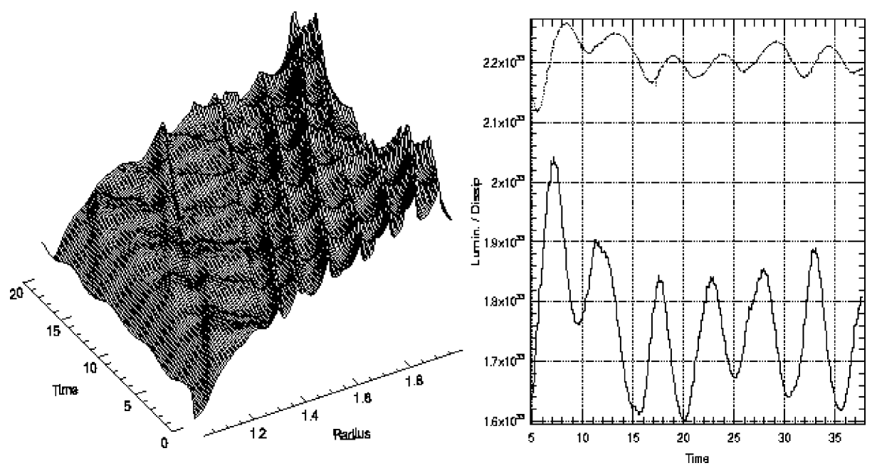
Figure 3: Time variation of the density for model 15 (a). Luminosity (dashed line) and total dissipation (solid line) versus time (b). value $\Omega_{k}$ and radial Mach number $|v|/c_{s}$ versus radius for the same model. Time given in dimensionless units with an offset.

object 3

However, highly unstable features remained in the boundary layers of the other two models (15, 16) with $\alpha=0.1.$ These features were not seen in the other models even when they showed signs of viscous overstability. Here the characteristic wavelength is much shorter and the temperature structure and power output are significantly affected in a highly irregular manner. The instability appears more pronounced with higher $c_{\rm v}/c_{\rm s}$, here the strongest instabilities are present for $c_{\rm v}/c_{\rm s}=0.5$. Then slightly supersonic speeds with shocks, as well as superviscous speeds occur. We remark that in the models with $\alpha=0.1$, the short wavelength inward coming compressional waves are not expected to be reflected at a Lindblad resonance before they reach the boundary layer region, so they are able to affect the power output there. This would indicate that if the outer boundary condition allows, waves may exist in the boundary layer region where they may significantly affect the power output. In Figure 3b the variation of the luminosity and the total dissipation is shown over a short time interval for model 15. The luminosity varies over timescales of the order of the dynamical time (orbital Keplerian period at the stellar surface) but the variations in amplitude are less than 4%.

Note that the driving mechanism for these motions is not just simple viscous overstability which was never seen in the boundary layer region. The generation of superviscous and sometimes supersonic speeds indicates that the nature of the causal description must play a role. In figure 3a the time variation of the density is displayed in a three-dimensional space time diagram. It is clear that there are quasi-periodic wave-like perturbances moving from the inside outwards which are generated in the vicinity of the boundary layer. The perturbations interact intricately with reflected waves moving inwards (Fig. 3a).

These waves occur in a region where the central temperatures lie somewhat below $10^{4}K$, where opacity rises rapidly with temperature. Hence, even though the central temperatures vary only very little, the effective temperature displays much stronger variations. The origin of the disturbances lies in an interaction of the radiative transport with the causal viscous transport. For higher $|v/c_{\rm s}|$, the interaction becomes very much stronger leading to variations in luminosity of a few percent in the case of model 15. Notice that models 13 and 15 have identical parameter $\alpha,\tau$, and $c_{\rm v}/c_{\rm s}$, and only differ in the mass inflow rate which is ten times higher in model 13. The increased disc thickness for the higher $\dot{M}$ model leads to a larger optical depth and higher temperatures that drive the system out of the instability region.

Acknowledgement: W. K. would like thank the Astronomy unit at QMW for their kind hospitality during two visits. This work was supported by the EC grant ERB-CHRX-CT93-0329.

References

- [1] Godon P.,1995, MNRAS, 274, 61.
- [2] Israel W., 1976, Annals of Physics, 100, 310.
- [3] Jou D., Casas-Vasquez J., Lebon G., 1993, Extended irreversible Thermodynamics, Springer-Verlag, Berlin 1993.
- [4] Kato S., 1978, MNRAS, 185, 629.
- [5] Kley W., 1989, A&A, 208, 98.
- [6] Kley W., Papaloizou J.C.B., Lin D.N.C., 1993, ApJ, 409, 739.
- [7] Lin D.N.C., Papaloizou J.C.B., 1985, in Protostars and Planets II, ed. D.C. Black & M.S. Mathes (Tucson: Univ. Arizona Press), 981. MNRAS, 168, 603.
- [8] Lynden-Bell D., Pringle J. E., 1974, MNRAS, 168, 603.
- [9] Narayan R., 1992, ApJ, 394, 261.
- [10] Popham R., Narayan R., 1991, ApJ, 370, 604.
- [11] Popham R., Narayan R., 1992, ApJ, 394, 255.
- [12] Pringle J. E., 1977, MNRAS, 178, 195.
- [13] Papaloizou J.C.B., Lin D.N.C., 1995, Ann. Rev. Astron. Astrophys., 33, 505.
- [14] Papaloizou J.C.B., Stanley G.Q.G., 1986, MNRAS, 220, 593.
- [15] Papaloizou J.C.B., Szuszkiewicz E., 1994, MNRAS, 268, 29.
- [16] Shakura N.I., Sunyaev R.A., 1973, A&A, 24, 337.
- [17] Syer D., Narayan R., 1993, MNRAS, 262, 749.