The Spectrum of Gravitational Wave Perturbations in the One-Bubble Open Inflationary Universe

Abstract

We give the initial spectrum of quantized gravitational waves in the context of the one-bubble open inflationary universe scenario. In determining the quantum state after the bubble nucleation we adopt the prescription to require the analyticity of positive frequency functions in half of the Euclidean extension of the background $O(3,1)$-symmetric spacetime. We find the spectrum is well behaved at the infrared limit and there appears no supercurvature mode. In the thin wall approximation, the explicit form of the spectrum of gravitational wave perturbations is calculated.

1 Introduction

The open inflationary universe scenario is one of exciting current topics among the physics in the early universe. The possibility to create an open universe $(\Omega_{0}<1)$ through bubble nucleation in the context of inflationary cosmology has become under discussion rather recently,[1, 2, 3, 4, 5, 6] and several models of inflaton potential have been proposed.[2, 4, 5, 6]

Now a central issue is if these models are compatible with the observed anisotropies of cosmic microwave background (CMB) on large angular scales. In several recent papers,[7, 8, 9, 10, 11, 12, 13, 14, 15] quantum fluctuations of the inflaton field that generate the initial curvature perturbations have been evaluated and the resulting spectrum of CMB anisotropies has been calculated. But a drawback of all the previous studies is that the gravitational degrees of freedom have not been taken into account.

The incorporation of gravitational perturbations causes two effects. One is the coupling between perturbations of the inflaton field and those of the metric, which may alter the spectrum of the initial curvature perturbations drastically. The other is the contribution of gravitational wave perturbations to the CMB anisotropy, which has not been taken into account at all in the previous analyses. As has been known, a constant time hypersurface in an open inflationary universe is not a Cauchy surface of the whole spacetime.[9] Thus we cannot set commutation relations on this hypersurface when we consider quantization of a field in the open universe. This difficulty has been solved in the case of a scalar field[9, 10] and recently a method to manage the gravitational wave modes in the Milne universe has been developed by the present authors[16] (Paper I).

In this paper, we extend the result in Paper I to make it applicable to a general open universe. The aim of this paper is to give the spectrum of gravitational wave perturbations in the context of the open inflationary universe scenario.

This paper is organized as follows. In section 2 we review the zeroth order approximation to an open universe model, which is based on the $O(4)-$symmetric bubble nucleation[17, 18], and explain the notation we use in the succeeding sections. In section 3 gravitational wave perturbations of the $O(4)-$symmetric bubble is investigated. First we show a similarity between the massless scalar field perturbation and the gravitational wave perturbation. Then using this similarity, we reinterpret the results for massless scalar field perturbations obtained in Ref. ST96 and give the spectrum of gravitational wave perturbations. Section 4 is devoted to summary and discussion.

In this paper, we use the units, $c=\hbar=1$, and adopt the metric signature, $(-,+,+,+)$.

2 Configuration of the $O(3,1)$-symmetric bubble

We consider the Einstein scalar model with a single real scalar field which has a potential, $V(\sigma)$, as shown in Fig. 1. The Lagrangian is given by

$${\cal L}=\sqrt{-g}\left[{1\over 2\kappa}R-{1\over 2}g^{\mu\nu}\partial_{\mu}\sigma\partial_{\nu}\sigma-V(\sigma)\right],$$ (1)

where $\kappa=8\pi G$, and $g$ and $R$ are the determinant of the metric tensor and the curvature scalar, respectively.

Figure 1: The potential of the scalar field

Here in this section, we review the background solution which represents the bubble nucleation.[17, 18] The conformal diagram of this solution is presented in Fig. 2. As shown in Fig. 2, we divide the whole spacetime into five regions. The upper right and the upper left triangle regions are labeled by $R$ and $L$, respectively. The central, diamond-shaped region that contains the bubble wall is labeled by $C$. In $C$, the background metric is written as

$$ds_{C}^{2}=dT^{2}+a^{2}(T)\left(-dr_{C}^{2}+\cosh^{2}r_{C}d\Omega^{2}\right),$$ (2)

and the scalar field depends only on “the cosmological time”, $T$,

$$\sigma=\sigma(T).$$ (3)

Then the equations of motion become

$$\ddot{\sigma}+3{\dot{a}\over a}\dot{\sigma}={dV(\sigma)\over d\sigma},$$ (4)

$$\left({\dot{a}\over a}\right)^{2}-{1\over a^{2}}={\kappa\over 3}\left({1\over 2}\dot{\sigma}^{2}-V(\sigma)\right),$$ (5)

where the dot $~{}\dot{~{}}~{}$ represents the derivative with respect to $T$.

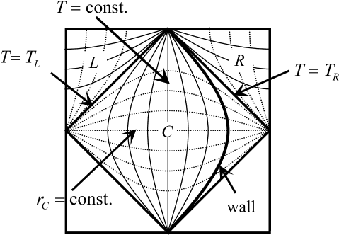
Figure 2: The conformal diagram of the universe containing an $O(3,1)$-symmetric bubble

The regularity of the metric requires the boundary condition for Eqs. (4) and (5) as

$$\dot{\sigma}|_{T=T_{J}}=0,$$ (6)

where $J=R$ or $L$ and $T_{J}$ is determined by $a(T_{J})=0$. Hereafter the subscript $J$ is used to represent $R$ or $L$. The surface where $T=T_{J}$ corresponds to the boundary between $C$ and $J$. As $T$ increases from $T_{L}$ to $T_{R}$, $\sigma$ also increases monotonically from $\sigma_{L}$ to $\sigma_{R}$. Here we assume that $\sigma_{L}$ is the potential minimum in the false vacuum side and that $\sigma_{R}$ is that in the true vacuum side. Further, we assume that the region in which $\sigma$ changes are restricted to the interval between $T_{WL}$ and $T_{WR}$, where $T_{WL}<T_{WR}$. We divide the region $C$ into three regions; $T<T_{WL}$, $T_{WL}<T<T_{WR}$ and $T_{WR}<T$, and call them $C_{L}$, $W$ and $C_{R}$, respectively. Thus $J$ and $C_{J}$ are the de Sitter space with $\sigma=\sigma_{J}$ with the expansion rate given by $H_{J}:=\sqrt{\kappa V(\sigma_{J})/3}$. As we shall see, these assumptions are not essential to our later discussion and they can be relaxed if one wishes. However, for simplicity, we consider the situation in which these assumptions hold.

Following Ref. ST96, we introduce coordinates in $L$ and $R$. First we introduce new coordinates in $C_{L}$ and $C_{R}$ by

$${dt_{C,J}\over H_{J}}=dT\raisebox{-5.0pt}{,}\quad a(T)={\cos t_{C,J}\over H_{J}}\raisebox{-5.0pt}{.}$$ (7)

In these coordinates, the metric in $C_{J}$ takes the form,

$$ds_{C,J}^{2}=H_{J}^{-2}\left[dt_{C,J}^{2}+\cos^{2}t_{C,J}\left(-dr_{C}^{2}+\cosh^{2}r_{C}d\Omega^{2}\right)\right].$$ (8)

If we use the thin wall approximation, in which the region $W$ is assumed to be infinitesimally thin, the continuity of the metric gives the relation,

$${\cos t_{C,L}\over H_{L}}\Bigr{|}_{wall}={\cos t_{C,R}\over H_{R}}\Bigr{|}_{wall}\,\raisebox{-5.0pt}{.}$$ (9)

Further we introduce the coordinates in $R$ and $L$ by

$$t_{R}=it_{C,R}-\pi i/2,\quad r_{R}=r_{C}+\pi i/2,$$ (10)

$$t_{L}=-it_{C,L}-\pi i/2,\quad r_{L}=r_{C}+\pi i/2.$$ (11)

The relations among the coordinate systems are uniquely determined by the analyticity which was discussed in Ref. YST96. The metric in $R$ or $L$ becomes

$$ds_{J}^{2}=H_{J}^{-2}\left[-dt_{J}^{2}+\sinh^{2}t_{J}\left(dr_{J}^{2}+\sinh^{2}r_{J}d\Omega^{2}\right)\right].$$ (12)

For later convenience, we introduce several symbols that describe background geometrical quantities. The expressions given here are valid in $R$ and $L$ but the extension to other regions is straightforward. We denote the unit vectors in $t$-direction and in $r$-direction as $\xi^{\mu}$ and $n^{\mu}$, respectively. Then the background metric can be decomposed as

$$g_{\mu\nu} = -\xi_{\mu}\xi_{\nu}+\gamma_{\mu\nu}$$ (13)

$$= -\xi_{\mu}\xi_{\nu}+n_{\mu}n_{\nu}+\sigma_{\mu\nu},$$ (14)

where $\gamma_{\mu\nu}$ and $\sigma_{\mu\nu}$ are the metric of the $t=\,$const. hypersurface and that of the $t,r=\,$const. surface, respectively. Further they are related to the metric of a unit 3-hyperboloid $\hat{\gamma}_{\mu\nu}$ and that of a unit 2-sphere $\hat{\sigma}_{\mu\nu}$ by

$$\gamma_{\mu\nu}=a^{2}\hat{\gamma}_{\mu\nu},\quad\sigma_{\mu\nu}=a^{2}\sinh^{2}r\,\hat{\sigma}_{\mu\nu}.$$ (15)

The small Latin indices such as $i$ and $j$ represent the projection; $f_{i}:=\gamma_{i}{}^{\mu}f_{\mu}$ and the vertical bar $|$ denotes the covariant derivative with respect to $\hat{\gamma}_{ij}$. The capital Latin indices such as $A$ and $B$ represent the projection; $f_{A}:=\sigma_{A}{}^{\mu}f_{\mu}$ and the double vertical bar $||$ denotes the covariant derivative with respect to $\hat{\sigma}_{AB}$.

3 Gravitational Wave Perturbations

We consider quantized gravitational wave perturbations on the background given in the preceding section. In general, the perturbed metric and the perturbed scalar field are given as

$$\tilde{g}_{\mu\nu}=g_{\mu\nu}+h_{\mu\nu}=g_{\mu\nu}+a^{2}~{}H_{\mu\nu},\quad\tilde{\sigma}=\sigma+\delta\sigma,$$ (16)

but here we ignore the perturbation of the scalar field and set $\delta\sigma=0$. Strictly speaking, one has to go to the region $C$, where a Cauchy surface exists, to quantize a field. For the metric perturbation, this is done in Appendix E for completeness. However, here we take a more intuitive approach by considering the metric perturbation in the region $R$ or $L$ first. For the present problem, it turns out this approach is as good as the rigorous one given in Appendix E.

In $R$ or $L$, we can impose the transverse traceless synchronous gauge condition on the metric perturbation. To make our statement explicit, we introduce the tensor harmonics on the 3-hyperboloid, $Y^{p\,lm}{}_{\mu\nu}=Y^{(+)p\,lm}{}_{\mu\nu}$ and $Y^{(-)p\,lm}{}_{\mu\nu}$, by [19]

$$Y^{(\pm)p\,lm}{}_{\mu\nu}\,\xi^{\nu}=0,$$

$$Y^{(+)p\,lm}{}_{ij}=\sqrt{(l-1)l(l+1)(l+2)\Gamma(ip+l+1)\Gamma(-ip+l+1)\over 2p^{2}(p^{2}+1)\Gamma(ip)\Gamma(-ip)}{\cal G}^{(+)p\,lm}_{ij},$$

$$Y^{(-)p\,lm}{}_{ij}=\sqrt{(l-1)(l+2)\Gamma(ip+l+1)\Gamma(-ip+l+1)\over 2l(l+1)(p^{2}+1)\Gamma(ip)\Gamma(-ip)}{\cal G}^{(-)p\,lm}_{ij},$$ (17)

where

$${\cal G}^{(+)p\,lm}_{rr}={\cal T}^{pl}_{1}Y\,,\quad{\cal G}^{(+)p\,lm}_{rA}={\cal T}^{pl}_{2}Y_{||A}\,,$$

$${\cal G}^{(+)p\,lm}_{AB}={\cal T}^{pl}_{3}Y_{||AB}+{\cal T}^{pl}_{4}Y{\hat{\sigma}_{AB}}\,,$$ (18)

$${\cal G}^{(-)}_{rr}=0,\quad{\cal G}^{(-)}_{rA}={\cal T}_{5}^{pl}{\cal Y}_{A},\quad{\cal G}^{(-)}_{AB}=2{\cal T}_{6}^{pl}{\cal Y}_{AB},$$ (19)

and $Y:=Y_{lm}(\Omega)$ are the 2-dimensional spherical harmonics and

$${\cal Y}_{A}:=Y_{||C}~{}\hat{\epsilon}^{C}_{~{}A},\quad{\cal Y}_{AB}:=Y_{||C(A}~{}\hat{\epsilon}^{C}_{~{}B)}=\ell(\ell+1)Y_{C(A}~{}\hat{\epsilon}^{C}_{~{}B)}\,.$$ (20)

The superscripts $(+)$ and $(-)$ denote parities of the harmonics and $\hat{\epsilon}_{AB}$ is the unit anti-symmetric tensor on the unit 2-sphere ($\hat{\epsilon}_{\theta\varphi}=\sin\theta$ etc.) and $\hat{\epsilon}^{A}{}_{B}=\hat{\sigma}^{AC}\hat{\epsilon}_{CB}$.

The $r$-dependent parts of the tensor harmonics are expressed in terms of the function,

$${\cal P}_{p\,l}(r):={P_{ip-{1\over 2}}^{-l-{1\over 2}}(\cosh r)\over\sqrt{\sinh r}},$$ (21)

as

$${\cal T}^{pl}_{1} = {1\over\sinh^{2}r}{\cal P}_{pl}(r)\,,$$

$${\cal T}^{pl}_{2} = {1\over l(l+1)}\left(\partial_{r}+{\coth r}\right){\cal P}_{pl}(r)\,,$$

$${\cal T}^{pl}_{3} = {2\sinh^{2}r\over(l-1)l(l+1)(l+2)}\left(\coth r\partial_{r}-\left\{p^{2}-1-{l(l+1)+2\over 2\sinh^{2}r}\right\}\right){\cal P}_{pl}(r)\,,$$

$${\cal T}^{pl}_{4} = {\sinh^{2}r\over(l-1)(l+2)}\left(\coth r\partial_{r}-\left\{p^{2}-1-{2\over\sinh^{2}r}\right\}\right){\cal P}_{pl}(r)\,,$$ (22)

$${\cal T}_{5}^{pl} = {\cal P}_{pl}(r),$$ (23)

$${\cal T}_{6}^{pl} = {\sinh^{2}r\over(l-1)(l+2)}\left(\partial_{r}+2\coth\,r\right){\cal P}_{pl}(r)\,,$$ (24)

where $P^{\mu}_{\nu}(z)$ is the associated Legendre function of the first kind. These harmonics satisfy spatial transverse traceless gauge condition:

$$Y^{p\,lm}{}_{ij}{}^{|j}=0,\quad Y^{p\,lm}{}_{i}{}^{i}=0,$$ (25)

and have the eigenvalue $p^{2}+3$ as

$$\left[{}^{(3)}\triangle+(p^{2}+3)\right]Y^{p\,lm}{}_{ij}=0,$$ (26)

where ${}^{(3)}\triangle$ is the tensor Laplacian operator on the unit 3-hyperboloid. Note that, by construction, there are no $l=0$ and $1$ modes in these harmonics. For positive $p^{2}$ modes, they are normalized as

$$\int d\Sigma~{}\hat{\gamma}^{ii^{\prime}}\hat{\gamma}^{jj^{\prime}}Y^{p\,lm}{}_{ij}\overline{Y^{p^{\prime}\,l^{\prime}m^{\prime}}{}_{i^{\prime}j^{\prime}}}=\delta(p-p^{\prime})\delta_{l,l^{\prime}}\delta_{m,m^{\prime}}\,,$$ (27)

where $d\Sigma=\sinh^{2}r\,drd\Omega$ is the surface element on the unit 3-hyperboloid. For negative $p^{2}$ modes, they are not normalizable. Thus it might be inappropriate to call them harmonics but we do so here and define them by Eq. (17).

Using the harmonics, we expand the metric perturbations as

$$H_{\mu\nu}=H_{(+)\mu\nu}+H_{(-)\mu\nu},$$ (28)

and

$$H_{(+)\mu\nu}=\sum_{p,l,m}U^{(+)}_{p\,lm}(t)Y^{(+)p\,lm}_{\mu\nu}(r,\Omega),$$ (29)

$$H_{(-)\mu\nu}=\sum_{p,l,m}U^{(-)}_{p\,lm}(t)Y^{(-)p\,lm}_{\mu\nu}(r,\Omega).$$ (30)

Then the perturbed Einstein equation in $C$ becomes

$$\left[{1\over a^{3}(T)}{d\over dT}a^{3}(T){d\over dT}+{p^{2}+1\over a^{2}(T)}\right]{U_{p\,lm}(T)}=0.$$ (31)

The equations in the other regions are obtained by the analytic continuation.

This equation is exactly the same one that was discussed in Ref. ST96 for a noninteracting massless scalar field without coupling to the metric perturbation. In the scalar case, we showed that there is one supercurvature mode ($p^{2}<0$) for each $l,m$ independent of the detail of the model under the thin wall approximation. With this result in mind, in the subsequent two sections, we discuss subcurvature modes ($p^{2}>0$) and supercurvature modes separately.

3.1 subcurvature modes

For subcurvature modes, the correspondence between the cases of the massless scalar perturbation and the gravitational wave perturbation is exact.

When $p^{2}>0$ the $r$-dependent parts of the harmonics vanish fast enough as $r\rightarrow\infty$. Therefore we can choose the union of a $t_{L}=\,$const. and a $t_{R}=\,$const. hypersurfaces as a surface on which the canonical commutation relations are set, although it is not a Cauchy surface.

As given in Appendix A, in $L$ and $R$, foliating the spacetime by $t_{J}=\,$const. hypersurfaces, the 2nd variation of the action becomes

$$\delta^{(2)}{\cal L}={1\over 8\kappa}\sum_{\sigma=\pm}\sum_{J=R,L}\int_{-\infty}^{+\infty}dp\sum_{l,m}\int d\tau_{J}\,a(\tau_{J})^{3}\left(\left|{dU^{(\sigma)}_{p\,lm}\over d\tau_{J}}\right|^{2}-{(p^{2}+1)\over a(\tau_{J})^{2}}|U^{(\sigma)}_{p\,lm}|^{2}\right),$$ (32)

where $\tau_{J}=t_{J}/H_{J}$. This action, for each definite parity, is the same as that of the massless scalar field $\phi$ with the decomposition,

$$\phi={1\over\sqrt{4\kappa}}\sum_{p,l,m}U_{p\,lm}(\tau)Y^{p\,lm}(r,\Omega),$$ (33)

where $Y^{p\,lm}(r,\Omega)$ is the normalized scalar harmonics on a unit 3-hyperboloid. The only difference is the presence of the $l=0$, $1$ modes in the scalar case. Then if we assume that the positive frequency functions of gravitational wave perturbations are determined by the same analyticity as in the case of the scalar field, the results obtained in Ref. ST96 can be reinterpreted for the present problem. Since the final expression for the amplitude of fluctuations of the scalar field, $\delta\phi$, was written in terms of the curvature perturbation ${\cal R}$ in Ref. ST96, it may be helpful to show here the relation;

$${\cal R}=-{H\over\dot{\phi}(t)}\delta\phi.$$ (34)

Then Eq. (23) of Ref. ST96 is reinterpreted to give the amplitude of the gravitational wave perturbations in the thin wall approximation:

$$\langle U_{p\,lm}^{2}\rangle={4\kappa H^{2}\coth\pi p\over 2p(1+p^{2})}(1-y),$$ (35)

where

$$1-y=1-{(\Delta s)^{2}\cos\tilde{p}+2p\Delta s\sin\tilde{p}\over\cosh\pi p\,(4p^{2}+(\Delta s)^{2})}\raisebox{-5.0pt}{,}$$ (36)

with $\Delta s:=\sin t_{C,R}|_{wall}-\sin t_{C,L}|_{wall}$ and

$$\tilde{p}=p\ln\left(\displaystyle{1+\sin t_{C,R}|_{wall}\over 1-\sin t_{C,R}|_{wall}}\right)\raisebox{-5.0pt}{.}$$ (37)

It is important to note that $1-y\propto p^{2}$ as $p\to 0$. Although we have adopted the thin wall approximation here, it is straightforward to extend the present analysis to the general case and our conclusion that $1-y\propto p^{2}$ as $p\to 0$ remains true.

As first pointed out by Allen and Caldwell,[21] if $y=0$, which would be the case for the pure de Sitter background, the even parity gravitational wave spectrum would have an infrared divergence in the limit $p\to 0$ because of the extra factor of $1/p^{2}$ in the normalization factor of the tensor harmonics (see Eq. (17)). However, as soon as the effect of the presence of the bubble is taken into account, this divergence disappears. Thus for a realistic model of one-bubble open inflation, the gravitational wave spectrum shows no pathological feature.

3.2 supercurvature modes

A supercurvature mode is a solution of Eq. (31) regular at both boundaries, $T=T_{R}$ and $T_{L}$, which may exist discretely at $p^{2}\leq 0$. Let us put aside the case of $p^{2}=0$ for a while. Then, as mentioned before, it was shown in Ref. ST96 under the thin wall approximation that there is only one supercurvature mode for each $l$ and $m$. It is a trivial solution $U(T)=\,$const. for $p^{2}=-1$. However, different from the massless scalar case, this supercurvature mode is unphysical in the present case because it turns out to be just a gauge degree of freedom as shown in Appendix B. Thus in the thin wall case, there is no supercurvature mode in the gravitational wave perturbations. In Appendix C, we prove the absence of the supercurvature modes in general without the thin wall approximation.

However, one might worry if the absence of supercurvature modes would depend on our choice of gauge. That is, a metric perturbation described by a singular solution of Eq. (31) could be transformed to a regular metric perturbation by a different choice of gauge. For $p^{2}<0$ but $p^{2}\neq-1$, using the mutual independence among the scalar, vector and tensor harmonics, it can be shown without trouble that such a gauge transformation do not exist.

For even parity $p^{2}=0$ modes, however, there is a problem that they become degenerate with scalar perturbation modes with $p^{2}=-4$.[8, 13, 11] Therefore, we must consider the scalar perturbation at the same time when discussing regularity of the metric. In Appendix D, we treat this problem and show that there exists no gauge transformation that makes the metric regular for even parity $p^{2}=0$ modes. Thus it is concluded that there exists no supercurvature modes for gravitational wave perturbations.

4 Summary and discussion

In this paper we have derived the spectrum of gravitational wave perturbations in the context of the open inflationary universe scenario. We have assumed that the quantum state after bubble nucleation is given by “the Euclidean vacuum state” that is determined by the analyticity of modes when they are continued to the Euclidean region. Under this assumption and in the thin wall approximation, we have explicitly obtained the spectrum (35). An important feature of the spectrum is that it is infrared finite as opposed to the case of pure de Sitter background. We have also found that there is no discrete spectrum that comes from supercurvature modes. At a glance, there seemed to exist supercurvature modes at $p^{2}=-1$ but it is shown to be an illusion due to gauge degrees of freedom.

A subtlety associated with the even parity $p^{2}=0$ modes that they become degenerate with the $p^{2}=-4$ scalar perturbation modes has been also resolved. Taking account of all the degrees of freedom of metric perturbations, we have shown that these modes do not exist. In the previous analyses[8, 13, 11] without taking into account the gravitational degrees of freedom, the scalar $p^{2}=-4$ modes occupied a special position because they existed independent of the detail of the potential of tunneling scalar field and were called wall fluctuation modes. Our result implies that these modes cease to exist once the gravitational degrees of freedom are taken into account. This result is consistent with that obtained by Kodama et al.[22] in the case of infinitely thin domain wall with vanishing potential energy in both vacua. We should note, however, that our result does not exclude the possibility that a discrete mode describing the wall fluctuation exists with a shifted eigenvalue other than $p^{2}=-4$.

Appendix A 2nd variation of the action

In this Appendix we derive 2nd variation of the action given in Eq. (32). Here we omit the subscript $J$ for simplicity.

Since we are interested only in the 2nd order variation, we compute the terms quadratic in $h_{\mu\nu}$ in the Einstein-Hilbert action:

$$\delta^{2}(\sqrt{-g}R) = (\delta^{2}\sqrt{-g}g^{\mu\nu})R_{\mu\nu}+(\delta\sqrt{-g}g^{\mu\nu})\delta R_{\mu\nu}+\sqrt{-g}g^{\mu\nu}\delta^{2}R_{\mu\nu}$$ (39)

$$= \sqrt{-g}\left(h^{\mu\rho}h_{\rho}{}^{\nu}-{1\over 2}hh^{\mu\nu}+\left({1\over 8}h^{2}-{1\over 4}h_{\rho\sigma}h^{\rho\sigma}\right)g^{\mu\nu}\right)R_{\mu\nu}$$

$$\quad-\sqrt{-g}(h^{\mu\nu}-{1\over 2}hg^{\mu\nu})\delta R_{\mu\nu}+\sqrt{-g}g^{\mu\nu}\delta^{2}R_{\mu\nu},$$

Now

$$\delta R_{\mu\nu} = (\delta\Gamma^{\rho}{}_{\mu\nu})_{;\rho}-(\delta\Gamma^{\rho}{}_{\mu\rho})_{;\nu}\,,$$ (40)

$$\delta^{2}R_{\mu\nu} = (\delta^{2}\Gamma^{\rho}{}_{\mu\nu})_{;\rho}-(\delta^{2}\Gamma^{\rho}{}_{\mu\rho})_{;\nu}+\delta\Gamma^{\sigma}{}_{\rho\sigma}\delta\Gamma^{\rho}{}_{\mu\nu}-\delta\Gamma^{\sigma}{}_{\rho\nu}\delta\Gamma^{\rho}{}_{\mu\sigma}\,.$$ (41)

Inserting these into Eq. (39) and using

$$\delta\Gamma^{\rho}{}_{\mu\nu}={1\over 2}(h^{\rho}{}_{\mu;\nu}+h^{\rho}{}_{\nu;\mu}-h_{\mu\nu}{}^{;\rho}),$$ (42)

we obtain the 2nd order variation of the Einstein-Hilbert action,

$$L_{G}^{(2)} = {1\over 2\kappa}{1\over\sqrt{-g}}\delta^{2}(\sqrt{-g}R)$$ (43)

$$\quad=L_{R}^{(2)}+{1\over 8\kappa}\left[-h_{\mu\nu;\rho}h^{\mu\nu;\rho}+2h_{\mu\nu;\rho}h^{\rho\mu;\nu}-2h_{\mu\nu}{}^{;\nu}h^{;\mu}+h_{;\mu}h^{;\mu}\right],$$

where

$$L_{R}^{(2)}={1\over 8\kappa}[\left(4h^{\mu\rho}h_{\rho}{}^{\nu}-{2}hh^{\mu\nu}\right)R_{\mu\nu}+\left({1\over 2}h^{2}-h_{\rho\sigma}h^{\rho\sigma}\right)R.$$ (44)

Noting that

$$R = 6\left({\ddot{a}\over a}+\left({\dot{a}\over a}\right)^{2}-{1\over a^{2}}\right),$$ (45)

$$R_{\mu\nu} = g_{\mu\nu}\left({\ddot{a}\over a}+2\left({\dot{a}\over a}\right)^{2}-{2\over a^{2}}\right)-2\xi_{\mu}\xi_{\nu}\left({\ddot{a}\over a}-\left({\dot{a}\over a}\right)^{2}+{1\over a^{2}}\right),$$ (46)

where $\xi^{\mu}$ is the unit vector normal to the $t=\,$constant hypersurface, we obtain

$$L_{R}^{(2)}= {1\over 8\kappa}\biggl{[}4\left(2h^{\mu\rho}h_{\rho}{}^{\nu}-hh^{\mu\nu}\right)\xi_{\mu}\xi_{\nu}\left(-{\ddot{a}\over a}-\left({\dot{a}\over a}\right)^{2}+{1\over a^{2}}\right)$$ (48)

$$+\left(h^{2}-2h_{\mu\nu}h^{\mu\nu}\right)\left({\ddot{a}\over a}-\left({\dot{a}\over a}\right)^{2}+{1\over a^{2}}\right)\biggr{]},$$

where the dot denote the derivative with respect to the cosmological time, $t/H$.

We also need the matter part of the Lagrangian:

$$L_{m}^{(2)} = {1\over\sqrt{-g}}\delta^{2}\left(\sqrt{-g}\left(-{1\over 2}g^{\mu\nu}\xi_{\mu}\xi_{\nu}\dot{\sigma}^{2}-V(\sigma)\right)\right),$$ (49)

$$= -{1\over 2}\left(2h^{\mu\rho}h_{\rho}{}^{\nu}-hh^{\mu\nu}\right)\xi_{\mu}\xi_{\nu}\dot{\sigma}^{2}+{1\over 8}\left(h^{2}-2h_{\mu\nu}h^{\mu\nu}\right)\left({1\over 2}\dot{\sigma}^{2}-V(\sigma)\right).$$ (50)

Then, using the equations of motion,

$$\left({\dot{a}\over a}\right)^{2}-{1\over a^{2}}={\kappa\over 3}\left({1\over 2}\dot{\sigma}^{2}+V(\sigma)\right),$$ (51)

$${\ddot{a}\over a}=-{\kappa\over 3}\left(\dot{\sigma}^{2}-V(\sigma)\right),$$ (52)

the summation of $L_{R}^{(2)}$ and $L_{m}^{(2)}$ simplifies to

$$L_{R}^{(2)}+L_{m}^{(2)}=-{1\over 8\kappa}\left(h^{2}-2h_{\mu\nu}h^{\mu\nu}\right)\left({\ddot{a}\over a}+2\left({\dot{a}\over a}\right)^{2}-{2\over a^{2}}\right).$$ (53)

Now, taking into account the facts that $h_{\mu\nu}\xi^{\nu}=0$ and $h=0$, the 2nd variation of the Lagrangian reduces to

$$L^{(2)} ={1\over 8\kappa}\biggl{[}2h_{ij}h^{ij}\left({\ddot{a}\over a}+2\left({\dot{a}\over a}\right)^{2}-{2\over a^{2}}\right)$$ (56)

$$\quad+\gamma^{\mu\mu^{\prime}}\gamma^{\nu\nu^{\prime}}\bigl{[}\xi^{\rho}\xi^{\rho^{\prime}}\left(h_{\mu\nu;\rho}h_{\mu^{\prime}\nu^{\prime};\rho^{\prime}}-4h_{\mu\nu;\rho}h_{\rho^{\prime}\mu^{\prime};\nu^{\prime}}\right)$$

$$\quad\quad+\gamma^{\rho\rho^{\prime}}\left(-h_{\mu\nu;\rho}h_{\mu^{\prime}\nu^{\prime};\rho^{\prime}}+2h_{\mu\nu;\rho}h_{\rho^{\prime}\mu^{\prime};\nu^{\prime}}\right)\biggr{]}.$$

The nonvanishing components of $h_{\mu\nu;\rho}$ are explicitly written as

$$h_{\mu\nu;\rho}~{}\xi^{\mu}\gamma^{\nu}{}_{i}\gamma^{\rho}{}_{j} = -{\dot{a}\over a}h_{ij},$$ (57)

$$h_{\mu\nu;\rho}~{}\gamma^{\mu}{}_{i}\gamma^{\nu}{}_{j}\xi^{\rho} = \dot{h}_{ij}-2{\dot{a}\over a}h_{ij},$$ (58)

$$h_{\mu\nu;\rho}~{}\gamma^{\mu}{}_{i}\gamma^{\nu}{}_{j}\gamma^{\rho}{}_{j} = h_{ij|k}.$$ (59)

Then using formulas of the $\Sigma$-integration of the harmonics

$$\int d\Sigma~{}{\hat{\gamma}^{ii^{\prime}}\hat{\gamma}^{jj^{\prime}}\hat{\gamma}^{kk^{\prime}}}Y^{p\,lm}{}_{ij|k}\overline{Y^{p^{\prime}\,lm}{}_{i^{\prime}j^{\prime}|k^{\prime}}} = (p^{2}+3)\delta(p-p^{\prime}),$$ (60)

$$\int d\Sigma~{}{\hat{\gamma}^{ii^{\prime}}\hat{\gamma}^{jj^{\prime}}\hat{\gamma}^{kk^{\prime}}}Y^{p\,lm}{}_{ij|k}\overline{Y^{p^{\prime}\,lm}{}_{k^{\prime}i^{\prime}|j^{\prime}}} = 3\delta(p-p^{\prime}),$$ (61)

we obtain the resulting formula (32).

Appendix B $p^{2}=-1$ mode

Looking at Eq. (31), it is easy to find that there is a trivial supercurvature mode solution at $p^{2}=-1$, which is given by $U(T)=\,$const.. Thus the corresponding metric perturbation is given by

$$h_{\mu\nu}\propto a^{2}{\cal G}_{\mu\nu},$$ (62)

where ${\cal G}_{\mu\nu}$ are the unnormalized harmonics on the unit 3-hyperboloid defined by Eqs. (18) and (19). In this Appendix, we show that this mode is not a physical one but a gauge mode.

To see this, we introduce the unnormalized vector harmonics on the unit 3-hyperboloid, ${\cal W}_{i}^{(\pm)p\,lm}$, which are defined by

$${\cal W}^{(+)p\,lm}_{r} = {\cal V}_{1}^{pl}Y,\quad{\cal W}^{(+)p\,lm}_{A}={\cal V}_{2}^{pl}Y_{||A},$$ (63)

$${\cal W}^{(-)p\,lm}_{r} = 0,\quad{\cal W}^{(-)p\,lm}_{A}={\cal V}_{3}^{pl}{\cal Y}_{A},$$ (64)

where $Y=Y_{lm}(\Omega)$ and ${\cal Y}_{A}$ is defined in Eq. (20). The $r$-dependent parts are

$${\cal V}_{1}^{pl}={1\over\sinh r}{\cal P},\quad{\cal V}_{2}^{pl}={1\over l(l+1)}\partial_{r}\left(\sinh r{\cal P}\right),\quad{\cal V}_{3}^{pl}={\sinh r}{\cal P},$$ (65)

where $\cal P$ is defined in Eq. (21). The harmonics satisfy

$$\left({}^{(3)}\triangle+p^{2}+2\right){\cal W}_{i}=0,$$ (66)

$${\cal W}_{i}{}^{|i}=0,$$ (67)

$$2{\cal W}_{(i|j)}{}^{|j}=-(p^{2}+4){\cal W}_{i},$$ (68)

$$\left({}^{(3)}\triangle+p^{2}+6\right){\cal W}_{(i|j)}=0.$$ (69)

From Eq. (68) one can see that the tensor constructed from the vector harmonics with $p_{v}^{2}=-4$ is transverse and traceless. Here we appended the subscript $v$ to $p$ to stress that it is the eigenvalue of the vector harmonics defined by Eq. (66). Thus ${\cal W}_{(i|j)}{(p_{v}^{2}=-4)}$ can be regarded as tensor harmonics. Comparing Eq. (69) with Eq. (26), the corresponding eigenvalue $p_{t}$ of the tensor harmonics is found as $p_{t}^{2}=p_{v}^{2}+3=-1$. In fact, we can calculate ${\cal W}_{(i|j)}$ explicitly as

$${\cal W}_{(i|j)}\hat{n}^{i}\hat{n}^{j} = \partial_{r}{\cal W}_{r},$$ (70)

$${\cal W}_{(i|j)}\hat{n}^{i}\sigma^{j}{}_{A} = {1\over 2}\left[\left(\partial_{r}-2\coth r\right){\cal W}_{A}+\partial_{A}{\cal W}\right],$$ (71)

$${\cal W}_{(i|j)}\sigma^{i}{}_{A}\sigma^{j}{}_{B} = {\cal W}_{(A|B)}+\hat{\sigma}_{AB}\sinh r\cosh r{\cal W}_{r},$$ (72)

where $\hat{n}^{i}$ is the unit normal in the $r$-direction on the unit 3-hyperboloid and $\sigma_{ij}=\hat{\gamma}_{ij}-\hat{n}_{i}\hat{n}_{j}$. Using the fact that

$${d\over dr}{{\cal P}{(p^{2}=-4)}\over\sinh r}=(l-1){{\cal P}{(p^{2}=-1)}\over\sinh^{2}r},$$ (73)

which follows from the derivative recursion relation of the associated Legendre functions, it can be verified that

$${\cal W}^{(+)}_{(i|j)}{(p^{2}=-4)} = (l-1){\cal G}^{(+)}_{ij}{(p^{2}=-1)},$$ (74)

$${\cal W}^{(-)}_{(i|j)}{(p^{2}=-4)} = {(l-1)\over 2}{\cal G}^{(-)}_{ij}{(p^{2}=-1)}.$$ (75)

Now we consider a purely spatial gauge transformation (infinitesimal coordinate transformation),

$$x^{\mu}\rightarrow x^{\mu}+\zeta^{\mu},$$ (76)

with $\zeta_{\mu}\xi^{\mu}=0$ and $\zeta_{\mu}\propto{\cal W}_{\mu}{(p^{2}=-4)}$. It gives the change of the metric;

$$2\zeta_{(\mu;\nu)}\xi^{\nu}=0,$$ (77)

$$2\zeta_{(i;j)}\propto a^{2}{\cal G}_{ij}(p^{2}=-1),$$ (78)

without disturbing the value of the scalar field. This is just the metric perturbation for the $p^{2}=-1$ mode given in Eq. (62).

Appendix C absence of supercurvature modes

Here we show that there exist no supercurvature modes in gravitational wave perturbations without using the thin wall approximation.

A supercurvature mode is a mode corresponding to a regular solution of Eq. (31) with $p^{2}\leq 0$. The problem to find a supercurvature mode is analogous to that to find a bound state in the quantum mechanics. Here, we note that a regular solution means the one that gives a regular metric perturbation. An inspection of Eq. (31) reveals that the solution behaves as $a^{-1\pm\Lambda}$ ($\Lambda=\sqrt{-p^{2}}$) for $p^{2}<0$ and as $a^{-1}$ or $a^{-1}\ln a$ for $p^{2}=0$ as $T\to T_{J}$. Then it can be shown that the metric perturbation is regular if the solution behaves as $a^{-1+\Lambda}$. Thus a supercurvature mode is an eigen mode that satisfies the boundary condition $U\to a^{-1+\Lambda}$ as $T\to T_{J}$.

First we introduce a new coordinate, $s$, defined by

$$dT=a^{3}ds,\quad a(s=0)=a_{max},$$ (79)

where $a_{max}$ is the maximum value of $a$ in C. Then Eq. (31) is rewritten as

$$\left[{d^{2}\over ds^{2}}+(p^{2}+1)a^{6}(s)\right]{U_{p\,lm}(s)}=0.$$ (80)

If there is a potential $Q(s)$ which satisfies

$$Q(s)\geq a^{6}(s)~{}~{}{\rm for}~{}{}^{\forall}s\,,\quad Q(s)>a^{6}(s)~{}~{}{\rm for}~{}{}^{\exists}s\,,$$ (81)

and if the equation

$$\left[{d^{2}\over ds^{2}}+(p^{2}+1)Q(s)\right]X=0,$$ (82)

has $N$ supercurvature modes (bound state solutions) with one of them at $p^{2}=0$, then the number of supercurvature modes of Eq. (80) is less than $N$.

Integrating the equations of motion (4), we obtain the following inequality:

$${1\over 2}\dot{\sigma}^{2}-V(\sigma(T)) = {1\over 2}(\dot{\sigma}|_{T=T_{max}})^{2}-V(\sigma(T_{max}))-3\int_{T_{max}}^{T}dT^{\prime}{\dot{a}\over a}\dot{\sigma}^{2}$$ (83)

$$\geq {1\over 2}(\dot{\sigma}|_{T=T_{max}})^{2}-V(\sigma(T_{max}))=:-{3\over\kappa}\tilde{H}^{2},$$ (84)

where the dot denotes the derivative with respect to $T$. The equality holds only for $T=T_{max}$. Then from Eq. (5), we find

$$\left({\dot{a}\over a}\right)^{2}-{1\over a^{2}}\geq-\tilde{H}^{2}.$$ (85)

Note that from the fact that the equality holds at $T=T_{max}$, i.e., at $s=0$, where $\dot{a}=0$, one finds

$$a_{max}=\tilde{H}^{-1}.$$ (86)

We introduce the scale factor $\tilde{a}$ of the de Sitter space with the radius $\tilde{H}^{-1}$. Then $\tilde{a}$ satisfies

$$\left({\dot{\tilde{a}}\over\tilde{a}}\right)^{2}-{1\over\tilde{a}^{2}}=-\tilde{H}^{2}.$$ (87)

Rewriting Eqs. (85) and (87) by using the $s$-coordinate, we obtain

$$A\left((\partial_{s}A)^{2}-1\right)\geq B\left((\partial_{s}B)^{2}-1\right),$$ (88)

where $A=1/2a^{2}$ and $B=1/2\tilde{a}^{2}$ and the equality holds only at $s=0$.

Now we prove that $A>B$, i.e., $a(s)<\tilde{a}(s)$ for ${}^{\forall}s$ except at $s=0$. Suppose $A\leq B$ at $s=s_{1}>0$. Then Eq. (88) tells us that $(\partial_{s}A)^{2}>(\partial_{s}B)^{2}$ because $A$ and $B$ are positive. Since $\partial_{s}A>0$ for $s>0$, this implies $\partial_{s}A>\partial_{s}B$. Therefore we would conclude that $B(s_{1})-A(s_{1})<B(s=0)-A(s=0)$. However, this contradicts with the fact $A(s=0)=B(s=0)=\tilde{H}^{2}/2$. Thus $A>B$ for $s>0$. A parallel discussion holds also in the case $s_{1}<0$. Thus we conclude that $A>B$ except at $s=0$.

Now if we set $Q(s)=\tilde{a}^{6}(s)$, the condition (81) is satisfied and Eq. (82) is equivalent to the equation to determine the mode function of a minimally coupled massless scalar field in the pure de Sitter space, which is known to have one supercurvature mode at $p^{2}=-1$ ($U=\,$const.) and one marginally regular mode at $p^{2}=0$ ($U\propto\dot{a}/a$). So Eq. (31) has only one supercurvature mode, which is the one at $p^{2}=-1$. But it was shown in Appendix B that this unique supercurvature mode is an illusion due to gauge degrees of freedom. Thus we conclude that there is no supercurvature mode in gravitational wave perturbations.

Appendix D $p^{2}=0$ modes

Here we consider the even parity $p^{2}=0$ modes by taking full account of the degeneracy between the scalar and tensor harmonics. Since it is natural to require that a physical mode should give regular metric and scalar field perturbations, we examine whether a regular solution exists in this degenerate case.

First we give the explicit relation between the scalar and tensor harmonics when they are degenerate. Let us introduce the unnormalized scalar harmonics on the unit 3-hyperboloid, ${\cal S}^{plm}={\cal P}_{pl}Y_{lm}$. They satisfy

$$\left({}^{(3)}\triangle+p^{2}+1\right){\cal S}=0,$$ (89)

$${\cal S}_{ij}{}^{|j}=-{2\over 3}(p^{2}+4){\cal S}_{|i}\,,$$ (90)

$$\left({}^{(3)}\triangle+p^{2}+7\right){\cal S}_{ij}=0\,,$$ (91)

where

$${\cal S}_{ij}:={\cal S}_{|ij}+{p^{2}+1\over 3}\hat{\gamma}_{ij}{\cal S}\,.$$ (92)

One readily sees ${\cal S}_{ij}$ is transverse-traceless when $p^{2}=-4$. Comparison of Eq. (91) with Eq. (26) immediately shows $p_{t}^{2}=p_{s}^{2}+4$, where $p_{t}$ and $p_{s}$ are the eigenvalues of the tensor and scalar harmonics, respectively. Hence the $p_{s}^{2}=-4$ modes are equivalent to tensor harmonics with $p_{t}^{2}=0$. Further by construction, it is clear that they have even parity. The explicit form of ${\cal S}_{ij}(p^{2}=-4)$ can be obtained by noting the fact,

$${d^{2}\over dr^{2}}{\cal P}(p^{2}=-4)={\cal P}(p^{2}=-4)+l(l-1){{\cal P}(p^{2}=0)\over\sinh^{2}r}\,.$$ (93)

Then we find

$${\cal S}_{ij}(p^{2}=-4)=l(l-1){\cal G}^{(+)}_{ij}(p^{2}=0),$$ (94)

where ${\cal G}^{(+)}_{ij}$ are given by Eq. (18). Thus it is necessary (and sufficient) to consider scalar type perturbations with $l\geq 2$ when discussing the even parity $p_{t}^{2}=0$ modes.

We consider the scalar type perturbations in region $R$ or $L$ and describe the perturbed metric as

$$d\tilde{s}^{2}=-(1+2A{\cal S})d\tau^{2}+2B{\cal S}_{|j}d\tau dx^{j}+a(t)^{2}\left\{(1+2H_{L}{\cal S})\hat{\gamma}_{ij}+2H_{T}{\cal S}_{ij}\right\}dx^{i}dx^{j}\,,$$ (95)

and the perturbed scalar field as

$$\tilde{\sigma}=\sigma+\varphi{\cal S}\,.$$ (96)

Then the field equation for $\varphi$ is given by

$$\ddot{\varphi} +3{\dot{a}\over a}\dot{\varphi}+{p^{2}+1\over a^{2}}\varphi+V^{\prime\prime}(\sigma)\varphi$$ (97)

$$-2A(\ddot{\sigma}+3{\dot{a}\over a}\dot{\sigma})-\dot{A}\dot{\sigma}+3\dot{H}_{L}\dot{\sigma}+{p^{2}+1\over a^{2}}B\dot{\sigma}=0.$$

The necessary components of the perturbed Einstein equations are the $(0,0)$, $(0,i)$ and the traceless part of $(i,j)$ components. They are given, respectively, as

$$2\left(3\left({\dot{a}\over a}\right)^{2}A-3{\dot{a}\over a}\dot{H}_{L}-{\dot{a}\over a}\,{p^{2}+1\over a^{2}}B-{p^{2}+4\over a^{2}}(H_{L}+{p^{2}+1\over 3}H_{T})\right)$$

$$\qquad\qquad=\kappa(A\dot{\sigma}-\dot{\sigma}\varphi-V^{\prime}\varphi)\,,$$ (98)

$$2\left({\dot{a}\over a}A-\dot{H}_{L}+{1\over a^{2}}B-{p^{2}+4\over 3}\dot{H}_{T}\right)=\kappa\dot{\sigma}\varphi\,,$$ (99)

$${1\over a}(a^{3}\dot{H}_{T})\dot{}\,-{1\over a}(aB)\dot{}\,-A-H_{L}-{p^{2}+1\over 3}H_{T}=0.$$ (100)

In order to solve the above set of equations, it is necessary to fix a gauge. For this purpose, let us consider a gauge transformation induced by an infinitesimal coordinate transformation,

$$\bar{\tau}=\tau+M{\cal S}\,,\quad\bar{x}^{i}=x^{i}+N{\cal S}^{|i}\,.$$ (101)

Then the perturbation variables transform as

$$\bar{A}=A-\dot{M}\,,$$

$$\bar{B}=B-a^{2}\dot{N}+M\,,$$

$$\bar{H}_{L}=H_{L}+{p^{2}+1\over 3}N-{\dot{a}\over a}M\,,$$

$$\bar{H}_{T}=H_{T}-N\,,$$

$$\bar{\varphi}=\varphi-\dot{\sigma}M\,.$$ (102)

Hence unless $\sigma$ is constant, which is the case of pure de Sitter background, one can choose a gauge in which $\varphi=H_{L}=0$ by using the above gauge degrees of freedom. Now specializing to the case of $p^{2}=-4$, one finds from Eqs. (98) and (99) that $A=0$ in this gauge. Then we find $B=0$ from the perturbed field equation (97). Thus the only remaining variable is $H_{T}$. From Eq. (100), we find it satisfies

$${1\over a^{3}}{d\over d\tau}(a^{3}{d\over d\tau}H_{T})+{1\over a^{2}}H_{T}=0\,.$$ (103)

Now going into the region $C$ by the identifications of $d\tau$ with $idT$ and $a$ with $ia$, we see that this equation exactly coincides with the one for the tensor $p^{2}=0$ modes given by Eq. (31).

Now let us examine the asymptotic behavior of the solution of Eq. (103) at $a\rightarrow 0$ in $C$. Noting that $a\sim|T-T_{J}|=:\Delta T$ near the boundaries, $H_{T}$ have regular and singular solutions which behave as $\Delta T^{-1}$ and $\Delta T^{-1}\ln\Delta T$, respectively. Since the statement given in Appendix C holds also in the present case, any solution is singular either at $T_{R}$ (boundary to the region $R$) or at $T_{L}$ (boundary to the region $L$). Thus we may conclude that there exists no discrete mode for $p^{2}=-4$ (i.e., no discrete even parity $p^{2}=0$ tensor mode) that would contribute to the quantum fluctuations.

However, it is not yet completely clear if the singular behavior of $H_{T}$ is real. It may be absorbed by a gauge transformation. Thus we have to show that there exists no gauge transformation that makes the metric and scalar field perturbations regular. The regularity can be examined by investigating the behavior of the perturbations as one approaches either of the two boundary light cones. Since the coordinates $T$ and $r_{C}$ are degenerate on the boundary light cone, it is necessary to evaluate the metric components in non-degenerate coordinates, e.g.,

$$\tilde{t}=\Delta T\cosh r_{C}\,,\quad\tilde{r}=\Delta T\sinh r_{C}.$$ (104)

Then the components are related by

$$\left(\begin{array}[]{c}\Delta T^{2}h_{TT}\\ \Delta Th_{Tr}\\ h_{rr}\end{array}\right)=\left(\begin{array}[]{ccc}\tilde{t}^{2}&2\tilde{t}\tilde{r}&\tilde{r}^{2}\\ \tilde{t}\tilde{r}&\tilde{t}^{2}+\tilde{r}^{2}&\tilde{t}\tilde{r}\\ \tilde{r}^{2}&2\tilde{t}\tilde{r}&\tilde{t}^{2}\end{array}\right)\left(\begin{array}[]{c}h_{\tilde{t}\tilde{t}}\\ h_{\tilde{t}\tilde{r}}\\ h_{\tilde{r}\tilde{r}}\end{array}\right).$$ (105)

When we take the limit to the boundary light cone, $\Delta T$ goes to $0$ while $\tilde{t}$ and $\tilde{r}$ stay finite. Thus it is required that the components, $\Delta T^{2}h_{TT}\sim\Delta T^{2}A{\cal S}$ and $\Delta Th_{Tr}\sim\Delta TB\partial_{r_{C}}{\cal S}$, should be regular. Since the radial part of ${\cal S}$ behaves as $\exp{(\sqrt{-p^{2}}-1)r_{C}}=\exp{r_{C}}\sim\Delta T^{-1}$, $\Delta TA$ and $B$ should be regular on the boundary light cone.

Now we know that it is sufficient to consider a solution that behaves as $H_{T}=\Delta T^{-1}\ln\Delta T$ at, say, the left boundary in $\varphi=A=B=H_{L}=0$ gauge. The gauge transformation (102) is still valid in region $C$ with replacements, $M\rightarrow iM$ and $B\rightarrow iB$. Thus we must set $N=\Delta T^{-1}\ln\Delta T$ in order to remove the singular behavior of $H_{T}$. Then $B$ becomes singular. To remove the singular behavior of $B$, we should take $M=-\ln\Delta T$. Then, however, $\varphi$ becomes singular as $-\dot{\sigma}\ln\Delta T\sim\Delta T\ln\Delta T$. The perturbation of scalar field itself is finite but the derivative diverges. Thus we finally conclude that no regular (hence physical) discrete mode exists.

Appendix E Canonically reduced action for gravitational wave perturbations

Here, we discuss the reduction of the action for gravitational wave perturbations in an open inflationary universe. We consider the metric perturbation in the region $C$, where a Cauchy surface exists, and take a canonical approach to reduce the degrees of freedom of the constrained system to the physical degrees of freedom. The discussion goes parallel to the case of gravitational waves in the Rindler universe given in Appendix A of Paper I. The case of the Rindler universe, in which the scale factor is set to $a(T)=T$, is one special example of general cases but almost all the equations which appeared in the Rindler case hold with replacements:

$$\chi\rightarrow r,\quad\partial_{\chi}\rightarrow\partial_{r},\quad\xi\rightarrow a(T),\quad\partial_{\xi}-{m\over\xi}\rightarrow\partial_{T}-m{\dot{a}\over a},\quad(m=0,1,2,\cdots),$$ (106)

$$(e)\rightarrow(+),\quad(o)\rightarrow(-),$$ (107)

where the dot $~{}\dot{~{}}~{}$ represents the derivative with respect to $T$. Thus we only show here the necessary changes other than these replacements. In this Appendix the subscript $C$ in $r_{C}$ is suppressed for notational simplicity.

The Lagrangian for gravitational wave perturbations is given in Eqs. (53) and (43). After analytic continuation to the region $C$, it becomes

$$L^{(2)}= {1\over 8\kappa}\left(h^{2}-2h_{\mu\nu}h^{\mu\nu}\right)\left({\ddot{a}\over a}+2\left({\dot{a}\over a}\right)^{2}-{2\over a^{2}}\right)$$ (109)

$$+{1\over 8\kappa}\left(-h_{\mu\nu;\rho}h^{\mu\nu;\rho}+2h_{\mu\nu;\rho}h^{\rho\mu;\nu}-2h_{\mu\nu}{}^{;\nu}h^{;\mu}+h_{;\mu}h^{;\mu}\right).$$

We adopt the convention to denote the projection of tensors as

$$f_{\xi} := f_{\mu}\,\xi^{\mu},$$ (110)

$$f_{n} := f_{\mu}\,n^{\mu}=a^{-1}f_{r}.$$ (111)

The relations,

$$n^{\mu}{}_{;\nu} = -{\dot{a}\over a}\xi^{\mu}n_{\nu}+{\tanh r\over a}\sigma^{\mu}{}_{\nu}\,,$$ (112)

$$\xi^{\mu}{}_{;\nu} = -{\dot{a}\over a}n^{\mu}n_{\nu}+{\dot{a}\over a}\sigma^{\mu}{}_{\nu}\,,$$ (113)

are used in the calculations below. Each component of covariant derivatives of the metric perturbation becomes

$$h_{nn;n} = {1\over a}\partial_{r}h_{nn}-2{\dot{a}\over a}h_{n\xi},\quad h_{nn;\xi}=\partial_{T}h_{nn},\quad h_{nn;A}=h_{nn||A}-{2\tanh r\over a}h_{nA},$$ (114)

$$h_{n\xi;n} = {1\over a}\partial_{r}h_{n\xi}-{1\over a}\left(h_{\xi\xi}+h_{nn}\right),\quad h_{n\xi;\xi}=\partial_{T}h_{n\xi},$$ (115)

$$h_{n\xi;A} = h_{n\xi||A}-{\tanh r\over a}h_{\xi A}-{\dot{a}\over a}h_{nA},\quad h_{\xi\xi;n}={1\over a}\partial_{r}h_{\xi\xi}-2{\dot{a}\over a}h_{n\xi},$$ (116)

$$h_{\xi\xi;\xi} = \partial_{T}h_{\xi\xi},\quad h_{\xi\xi;A}=h_{\xi\xi||A}-2{\dot{a}\over a}h_{\xi A},$$ (117)

$$\quad h_{nA;n} = {1\over a}\left(\partial_{r}-\tanh r\right)h_{nA}-{\dot{a}\over a}h_{\xi A},\quad h_{nA;\xi}=\left(\partial_{T}-{\dot{a}\over a}\right)h_{nA},$$ (118)

$$h_{nA;B} = h_{nA||B}+\left({\dot{a}\over a}h_{n\xi}-{\tanh r\over a}h_{nn}\right)\sigma_{AB}-{\tanh r\over a}h_{AB},$$ (119)

$$h_{\xi A;n} = {1\over a}\left(\partial_{r}-\tanh r\right)h_{\xi A}-{\dot{a}\over a}h_{nA},\quad h_{\xi A;\xi}=\left(\partial_{T}-{\dot{a}\over a}\right)h_{\xi A},$$ (120)

$$h_{\xi A;B} = h_{\xi A||B}+\left({\dot{a}\over a}h_{\xi\xi}-{\tanh r\over a}h_{n\xi}\right)\sigma_{AB}-{\dot{a}\over a}h_{AB},$$ (121)

$$h_{AB;n} = {1\over a}\left(\partial_{r}-2\tanh r\right)h_{AB},\quad h_{AB;\xi}=\left(\partial_{T}-2{\dot{a}\over a}\right)h_{AB},$$ (122)

$$h_{AB;C} = h_{AB||C}+\left(2{\dot{a}\over a}h_{\xi(A}\sigma_{B)C}-{2\tanh r\over a}h_{n(A}\sigma_{B)C}\right),$$ (123)

where we used the abbreviated notation such as $h_{nA;\xi}\equiv h_{\mu\nu;\rho}n^{\mu}\sigma^{\nu}_{~{}A}\xi^{\rho}$. Below we expand the metric perturbation in terms of the spherical harmonics and consider the even and odd parity modes separately.

E.1 even parity

Concentrating on the even parity modes, we expand the variables by using the spherical harmonics $Y=Y_{\ell m}(\Omega)$,

$$h^{(+)}_{nn}=\sum H^{(+)\ell m}_{nn}Y,\quad h^{(+)}_{n\xi}=\sum H^{(+)\ell m}_{n\xi}Y,\quad h^{(+)}_{\xi\xi}=\sum H^{(+)\ell m}_{\xi\xi}Y,$$ (124)

$$h^{(+)}_{nA}=\sum H^{(+)\ell m}_{n}Y_{||A},\quad h^{(+)}_{\xi A}=\sum H^{(+)\ell m}_{\xi}Y_{||A},$$ (125)

$$h^{(+)}_{AB}=\sum\left(w^{(+)\ell m}Y\hat{\sigma}_{AB}+v^{(+)\ell m}Y^{(s)}_{AB}\right),$$ (126)

where

$$Y^{(s)}_{AB}={Y_{||AB}\over\ell(\ell+1)}+{1\over 2}\hat{\sigma}_{AB}Y.$$ (127)

Then the same argument that are given below Eq. (A8) of Paper I holds with the replacements listed in Eq. (107) and the action can be reduced under the synchronous gauge condition. Finally we obtain the reduced action:

$$\int dr\int dT~{}{\cal L}^{(+)}_{(red)}=\sum_{\ell,m}{8\over(\ell-1)\ell(\ell+1)(\ell+2)}\int dr\int{dT\over a^{3}}\Biggl{[}\overline{\Pi}\hat{K}(\hat{K}-1)\left(\partial_{r}w\right)$$ (129)

$$-{1\over 2}\left({1\over\cosh^{2}r}\overline{\Pi}\hat{K}(\hat{K}-1)\Pi+\overline{w}\hat{K}(\hat{K}-1)\left\{\ell(\ell+1)+\hat{K}\cosh^{2}r\right\}w\right)\Biggr{]},$$

where $\Pi$ is defined by

$$\Pi^{(+)\ell m}:=-\cosh^{2}r\left[{\ell(\ell+1)a\over 2}H^{(+)\ell m}_{n}+\tanh r~{}w^{(+)\ell m}\right],$$ (131)

and $\hat{K}$ is the derivative operator defined by

$$\hat{K}=-a\partial_{T}a^{3}\partial_{T}a^{-2}.$$ (132)

To keep the simplicity of notation, we often abbreviate the indices, $(\pm),\ell$ and $m$, unless there arises confusion.

Then we can see easily that $w$ and $\Pi$ can be expanded in terms of the eigen function of the operator $\hat{K}$. The normalized eigen functions should satisfy

$$\hat{K}{\cal U}_{p}(T)=(p^{2}+1){\cal U}_{p}(T),$$ (133)

and

$$\int_{T_{L}}^{T_{R}}{dT\over a^{3}}{\cal U}_{p}\overline{{\cal U}_{p^{\prime}}}=\left\{\begin{array}[]{cc}\delta(p-p^{\prime}),&(p^{2}\geq 0),\\ \displaystyle\sum_{n}\delta_{p,p_{n}}\delta_{p^{\prime},p_{n}},&(p^{2}<0).\end{array}\right.$$ (134)

where $p_{n}^{2}+1$ is a discrete eigenvalue of the operator $\hat{K}$. We expand the variables $w$ and $\Pi$ as

$$w^{(+)\ell m}=-\int dp~{}w_{(+)p\ell m}{\cal U}_{p},\quad\Pi^{(+)\ell m}=-\int dp~{}\Pi_{(+)p\ell m}{\cal U}_{p}.$$ (135)

As we adopt the synchronous gauge condition, we can write down the mode functions by using the tensor harmonics as

$$h_{ij}=\sum{\cal N}_{(+)pl\,m}{\cal U}_{p}(T){\cal G}_{ij}^{(+)pl\,m},$$ (136)

where ${\cal N}_{(+)pl\,m}$ is a normalization constant to be determined later. Then comparison of the traceless part of $h^{(+)p\ell m}_{AB}$ with the definition of $w$ in Eq. (126) readily gives the solution for $w_{(+)p\ell m}(r)$,

$$w_{(+)p\ell m}=-{{\cal N}_{(+)p\ell m}\over 2}{\cal P}_{p\ell}\,,$$ (137)

which, of course, satisfies the equation of motion which follows from the reduced action (LABEL:redact). Then repeating the same discussion succeeding to Eq. (A37) of Paper I, the normalization is found to be fixed as

$${\cal N}_{(+)pl\,m}=\sqrt{(l-1)l(l+1)(l+2)\Gamma(ip+l+1)\Gamma(-ip+l+1)\over 4p^{2}(p^{2}+1)}.$$ (138)

For $p^{2}>0$, taking account of the fact that the normalization of ${\cal U}_{p}$ defined by Eq. (134) gives rise to an additional factor $2/|\Gamma(ip)|^{2}$ when their Klein-Gordon norms are evaluated on hypersurfaces in $R$ and $L$ (see Appendix A of Ref. STY95), we can see that the same normalization is deduced from the action (32).

As for $p^{2}<0$, the normalization constant (138) is finite except for the case $p^{2}=-1$. Hence the supercurvature modes would exist if there were modes of ${\cal U}_{p}$ that would satisfy the normalization condition (134). But we know that such modes do not exist from the discussion of Appendix C.

In the case $p^{2}=-1$, the normalization constant ${\cal N}_{(+)pl\,m}$ diverges. On the other hand, since ${\cal U}_{p}\propto a^{2}$ for $p^{2}=-1$, the integral,

$$I_{p}^{2}=\int_{T_{L}}^{T_{R}}{dT\over a^{3}}|{\cal U}_{p}|^{2},$$ (139)

is finite. Hence the overall normalization factor, which is given by ${\cal N}_{(+)pl\,m}/I_{p}$, diverges. This implies the $p^{2}=-1$ modes are ‘zero modes’ for which the potential in the configuration space along the direction of the modes is flat. As shown in Appendix B, this corresponds to the fact that the $p^{2}=-1$ modes are gauge illusion and there is no dynamical degree of freedom there. So we do not have worry about this case.

Another case of the divergent ${\cal N}_{(+)pl\,m}$ occurs at the boundary between the subcurvature and supercurvature modes, $p^{2}=0$. In this case, however, an analysis of the asymptotic behavior of ${\cal U}_{p}$ as $T\to T_{J}$ ($J=L,R$) shows the integral (139) diverges as well. Therefore the overall normalization factor ${\cal N}_{(+)pl\,m}/I_{p}$ becomes indefinite as $\infty/\infty$ and we cannot conclude there is no physical discrete mode there. This case is special in the sense that the even parity $p^{2}=0$ tensor harmonics can be constructed from the $p^{2}=-4$ scalar harmonics[8, 13, 11]. Thus these modes are degenerate with scalar type perturbations in the language of cosmological perturbation theory and a complete treatment can be done only if the perturbation of the scalar field is taken into account at the same time. Such an analysis has been given in Appendix D and it has been shown that there exists no physical discrete mode at $p^{2}=0$.

E.2 odd parity

We expand the metric perturbation in terms of the spherical harmonics as

$$h^{(-)}_{nA}=\sum H^{(-)\ell m}_{n}{\cal Y}_{A},\quad h^{(-)}_{\xi A}=\sum H^{(-)\ell m}_{\xi}{\cal Y}_{A},\quad h^{(-)}_{AB}=\sum w^{(-)\ell m}{\cal Y}_{AB}\,.$$ (140)

As in the even parity case, the same argument below Eq. (A49) of Paper I holds with the replacements listed in Eq. (107).

Finally we obtain the reduced action:

$$\int dr\int dT~{}{\cal L}^{(-)}_{(red)}=\sum_{\ell,m}{2\ell(\ell+1)\over(\ell-1)(\ell+2)}\int dr\int{dT\over a^{3}}\Biggl{[}\Pi\hat{K}\left(\partial_{r}Q\right)$$ (142)

$$-{1\over 2}\left({1\over\cosh^{2}r}\overline{\Pi}\hat{K}\Pi+\overline{Q}\hat{K}\left\{\ell(\ell+1)+\hat{K}\cosh^{2}r\right\}Q\right)\Biggr{]},$$

where

$$Q^{(-)\ell m} := aH^{(-)\ell m}_{n}$$ (143)

$$\Pi^{(-)\ell m} := -{\ell(\ell+1)-2\over 2}w^{(-)\ell m}-2a\sinh r\cosh rH^{(-)\ell m}_{n}.$$ (144)

As before, the variables $Q$ and $\Pi$ are expanded as

$$Q^{(-)\ell m}=-a^{2}\int dp~{}Q_{(-)p\ell m}{\cal U}_{p},\quad\Pi^{(-)\ell m}=-a^{2}\int dp~{}\Pi_{(-)p\ell m}{\cal U}_{p}\,.$$ (145)

We write down the mode functions by using the tensor harmonics as

$$h_{ij}=a^{2}\sum{\cal N}_{(-)pl\,m}{\cal U}_{p}(T){\cal G}_{ij}^{(-)pl\,m}.$$ (146)

Then comparison of $h^{(-)p\ell m}_{rA}$ with the definition of $Q$ gives

$$Q_{(-)p\ell m}=-{{\cal N}_{(-)p\ell\,m}}{\cal P}_{p\ell}\,,$$ (147)

Then as in the case of even parity modes the normalization is fixed as

$${\cal N}_{(-)pl\,m}=\sqrt{(l-1)(l+2)\Gamma(ip+l+1)\Gamma(-ip+l+1)\over 4l(l+1)(p^{2}+1)}.$$ (148)

Different from even parity modes, the only exceptional case is the $p^{2}=-1$ modes. But again they are unphysical as shown in Appendix B. Thus there exists no physical discrete modes.

References

[1]
J. R. Gott III, Nature 295, 304 (1982);
J. R. Gott III and T. S. Statler, Phys Lett 136B, 157 (1984).
[2] M. Bucher, A. S. Goldhaber and N. Turok,
Nucl. Phys. B, Proc. Suppl. 43, 173 (1995);
M. Bucher, and N. Turok, Phys. Rev. D 52, 5538 (1995).
[3] K. Yamamoto, M. Sasaki and T. Tanaka,
Astrophys. J. 455, 412 (1995).
[4] A. D. Linde, Phys. Lett. B 351, 99 (1995).
[5] A. D. Linde and A. Mezhlumian, Phys. Rev. D 52,
5538 (1995).
[6] A. M. Green and A. R. Liddle, report No.
SUSSEX-AST 96/7-7, astro-ph/9607166.
[7]
K. Yamamoto, T. Tanaka, and M. Sasaki, Phys. Rev. D 51,
2968 (1995).
[8]
T. Hamazaki, M. Sasaki, T. Tanaka, and K. Yamamoto,
Phys. Rev. D 53 2045 (1996).
[9] M. Sasaki, T. Tanaka, and K. Yamamoto,
Phys. Rev. D 51, 2979 (1995).
[10]
M. Sasaki and T. Tanaka, Phys. Rev. D 54, 4705 (1996).
[11]
K. Yamamoto, M. Sasaki and T. Tanaka, Phys. Rev. D 54, 5031 (1996).
[12]
K. Yamamoto and E. F. Bunn, Astrophys. J. 464, 8 (1996).
[13]
J. Garriga, Phys. Rev. D 54, 4764 (1996).
[14]
J. Garcia-Bellido, Phys. Rev. D 54, 2473 (1996).
[15]
J. D. Cohn, Reprot No. LBNL-38560, UCB-PTH-96/10, astro-ph/9605132,
to appear in Phys. Rev. D 54 (1996).
[16]
T. Tanaka and M. Sasaki, Report No. OU-TAP 45, gr-qc/9610060, (Paper I).
[17] S. Coleman, Phys. Rev. D 15, 2929 (1977).
[18] S. Coleman and F. De Luccia, Phys. Rev. D 21
3305 (1980).
[19]
K. Tomita, Prog. Theor. Phys. 68, 310 (1982).
[20] T. Tanaka and M. Sasaki, Phys. Rev. D 50,
6444 (1994).
[21] B. Allen and R. Caldwell, Report No. WISC-MILW-94-TH-21.
[22]
H. Kodama, H. Ishihara and Y. Fujiwara,
Phys. Rev. D 50, 7292 (1994).