Energy Budget and the Virial Theorem in Interstellar Clouds

Abstract

The Virial Thoerem (VT) is a mathematical expression obtained from the equation of motion for a fluid, which describes the energy budget of particular regions within the flow. This course reviews the basic theory leading to the VT, discusses its applicability and limitations, and then summarizes observational results concerning the physical and statistical properties of interstellar clouds which are normally understood in terms of the VT, in particular the so-called “Larson’s Relations”. In all cases, the standard notions as well as relevant counterpoint are presented. In particular, the difficulties arising when the medium is fully turbulent are discussed.

To appear in “Millimetric and Sub-Millimetric Astronomy. INAOE 1996 Summer School”.

1. Introduction

The interstellar medium is an extremely complex mixture of gas, dust, and cosmic rays, threaded by a ubiquitous magnetic field, and stirred by a wide variety of energy sources such as supernovae, expanding HII regions and bipolar outflows. Progressively higher-density regions in this medium constitute what we normally call intercloud medium, cloud complexes, diffuse clouds, molecular clouds, clumps and cores, respectively, although the boundaries between these classifications are fuzzy (a natural consequence of drawing arbitrary classification boundaries in a continuum). Table 1 gives the ranges of densities and temperatures for the above structures (adapted from Jura 1987).

Table 1.: Structures in the interstellar medium.
(Adapted from Jura 1987.)

Name	$n({\rm cm}^{-3})$	$T$(K)	Filling factor
Hot intercloud	$3\times 10^{-3}$	$10^{6}$	$0.1-0.7$?
gas
Warm gas	$0.1$	$10^{3}-10^{4}$	$0.4$
Diffuse clouds	$<10$	$50-100$
Cirrus clouds	$10-10^{3}$	$10-100$
Dark clouds	$>10^{3}$	$10$	$0.01$?
GMCs	$>10^{3}$	$15-40$
H II regions	$>10$	$10^{4}$
SNR	$>1$	$10^{4}-10^{7}$

The gaseous component of this medium should be reasonably well described as a compressible, self-gravitating fluid (e.g, Shu 1992, Ch. 1) obeying the magnetohydrodynamic (MHD) equations, since even very low ionization fractions allow coupling of the motions to the magnetic field (Mestel & Spitzer 1956; see also Shu 1992, Ch. 27). From one of these equations, a very important result called the Virial Theorem (VT) can be obtained, which describes the energy balance (or “budget”) of particular regions within the medium. In this course, we first review the derivation of the VT (§ 2.), stressing in particular the physical meaning of each term, including the often-neglected surface terms, and the validity of frequently used simplifying assumptions (e.g., Shu 1992). In § 3. we then discuss various applications of the Virial Theorem, both to idealized cases and to real interstellar cloud properties, pointing out existing incompletenesses. Finally, in § 4. contains the conclusions. Throughout this course, we shall ignore the flux-loss effects of ambipolar diffusion (e.g, Shu 1992).

2. The MHD Equations and the Virial Theorem

2.1. The MHD equations

In order for the gaseous component of the ISM to be adequately described by a continuum approximation, it is necessary that the mean free paths of the gas molecules be much smaller than the characteristic length scale of the systems under consideration (e.g., Currie 1974). This is generally satisfied in most kinds of interstellar structures, since the characteristic length scales are normally at least some $10^{5}$ times larger than the mean free paths (e.g., Shu 1992). The use of the MHD equations is thus amply justified. These equations, describing the evolution of a magnetized, compressible gas without dissipative terms, are (e.g., Cowling 1976; Spitzer 1978; Shu 1992; Shore 1992):

i) The Continuity Equation, expressing mass conservation:

$${\partial\rho\over\partial t}+{\nabla}\cdot(\rho{\bf u})=0;$$ (1)

ii) The Momentum Balance Equation

$${\rho\partial{\bf u}\over\partial t}+\rho{\bf u}\cdot\nabla{\bf u}=-{\nabla P}-\rho\nabla\varphi+{1\over 4\pi}\bigl{(}\nabla\times{\bf B}\bigr{)}\times{\bf B}-2\rho\Omega\times{\bf u};$$ (2)

iii) The Internal Energy Balance Equation

$${\partial e\over\partial t}+{\bf u}\cdot\nabla e=-(\gamma-1)e\nabla\cdot{\bf u}+\Gamma-\rho\Lambda;$$ (3)

iv) The Magnetic Field Equation (flux freezing)

$${\partial{\bf B}\over\partial t}=\nabla\times({\bf u}\times{\bf B});$$ (4)

v) Poisson’s Equation

$$\nabla^{2}\varphi=4\pi G\rho.$$ (5)

Additionally, we assume an ideal-gas equation of state $P=(\gamma-1)\rho e$.

In these equations, $\rho$ is the mass density of the gas, u is the fluid velocity, $P$ is the thermal pressure, $e$ is the specific internal energy, B is the magnetic field, and $\varphi$ is the gravitational potential. Additionally, $\Gamma$ and $\Lambda$ symbolically represent any heating and cooling sources present in the medium, and are normally functions of the density and temperature in the MHD description (neglecting radiative transfer and chemical composition).

Let us now briefly discuss the meaning of the main terms in these equations. In eq. (2), which is Newton’s Second Law in per-unit-volume form, the second term on the left hand side (LHS) is the so-called non-linear or advective term, and expresses the momentum transport by the velocity field itself. This is the term that describes the effects of turbulence in the medium. The first term in the right hand side (RHS) gives the force (per unit volume) exerted by the thermal pressure gradient. The second term is the self-gravitational force, the third term is the Lorentz force, and the last term is the Coriolis force, due to Galactic rotation with an angular velocity $\Omega$.

In eq. (3), the second term on the LHS expresses internal energy transport by the velocity field (convection). The first term on the RHS is the $PdV$ work. In eq. (4), the RHS is the flux freezing condition, implying that magnetic field lines are dragged along with the matter. Finally, eq. (5) expresses that the source of the gravitational potential is the mass density.

Important physics left out from this description are, as mentioned above, the radiative transfer and the chemical and ionization fraction evolution. These can be crudely incorporated in the equations above by means of model terms, such as $\Gamma$ and $\Lambda$ in eq. (3), or by making the equation of state vary in different regimes. This allows an approximate description of the effects of these processes on the dynamics, although it cannot allow any predictions on those processes themselves. Finally, note that the MHD equations hold in the so-called “MHD approximation” which assumes an conductivity of the medium.

2.2. The Virial Theorem

The scalar VT is obtained by dotting the momentum equation (eq. 2) with the position vector x and integrating over some volume $V$. Traditionally, the volume $V$ is taken in a Lagrangian frame of reference moving with the fluid (e.g., Spitzer 1978; Shu 1992). An Eulerian (i.e, in a fixed frame of reference) version of the VT has recently been derived by McKee & Zweibel (1992, hereafter MZ92). This may be a more convenient form for computation in practice (e.g., MZ92; Ballesteros-Paredes & Vázquez-Semadeni 1997), but here we discuss the Lagrangian version for consistency with most treatments. Neglecting the Coriolis force, which is negligible at molecular cloud scales, one obtains

$$\int_{V}\rho{\bf x}\cdot{d{\bf u}\over dt}dV=-\int_{V}{\bf x}\cdot\nabla PdV-\int_{V}\rho{\bf x}\cdot\nabla\varphi dV+{1\over 4\pi}\int_{V}{\bf x}\cdot(\nabla\times{\bf B})\times{\bf B}dV,$$ (6)

where $d/dt=\partial/\partial t+{\bf u}\cdot\nabla$ is the total or Lagrangian derivative operator. The LHS can be rewritten as

$$\int_{V}\rho{\bf x}\cdot{d{\bf u}\over dt}dV={1\over 2}\int{d^{2}x^{2}\over dt^{2}}dm-\int_{V}\rho u^{2}dV\equiv{1\over 2}{d^{2}I\over dt^{2}}-\int_{V}\rho u^{2}dV,$$ (7)

where we have defined $dm=\rho dV$, and have used Reynolds’ Transport Theorem

$${d\over dt}\int_{V}\alpha dV=\int_{V}\Bigl{[}{\partial\alpha\over\partial t}+\nabla\cdot(\alpha{\bf u})\Bigr{]}dV$$ (8)

to show that ${d\over dt}\int\alpha dm=\int{d\alpha\over dt}dm$. Also, the second equality in eq. (7) defines the moment of inertia $I$.

For the RHS, consider the following. First, according to Newton’s Law of Gravitation (or from the solution of Poisson’s equation) the gravitational term can be written as

$$W\equiv-\int_{V}\rho({\bf x}){\bf x}\cdot\nabla\varphi dV=-G\int_{V}\int_{\rm all\ space}{\rho({\bf x})\rho({\bf x}^{\prime}){\bf x}\cdot({\bf x}-{\bf x}^{\prime})\over|{\bf x}-{\bf x}^{\prime}|^{3}}dV^{\prime}dV.$$ (9)

Noting that the integrand is nearly symmetric with respect to the primed and unprimed variables, we can replace x by $({\bf x}-{\bf x}^{\prime})/2$ and write

$$W=-{1\over 2}G\int_{V}\int_{\rm all\ space}{\rho({\bf x})\rho({\bf x}^{\prime})\over|{\bf x}-{\bf x}^{\prime}|}dVdV^{\prime}.$$ (10)

Thus, $W$ is the gravitational energy of the mass distribution within volume $V$, given the mass distribution of the whole space. Note that in Shu (1992), both integrals are evaluated over volume $V$. This approximation is valid only if the mass outside volume $V$ can be neglected (see Spitzer 1978), a fact which is often overlooked.

Secondly, the remaining thermal pressure and magnetic terms can be dealt with using Gauss’ divergence theorem, and the facts that $\nabla\cdot{\bf x}=3$ and that (in tensor notation) $\partial x_{i}/\partial x_{j}=\delta_{ij}$. Additionally, for the magnetic term, it is most convenient to work with Maxwell’s magnetic stress tensor ${\bf T}\equiv T_{ij}\equiv B_{i}B_{j}/4\pi-|{\bf B}|^{2}\delta_{ij}/8\pi$, such that the flux freezing term satisfies $(\nabla\times{\bf B})\times{\bf B})/4\pi=\nabla\cdot T_{ij}$. Thus, the VT finally reads

$${1\over 2}{d^{2}I\over dt^{2}}=\int\rho u^{2}dV+\Bigl{(}3\int PdV-\oint_{S}P{\bf x}\cdot d{\bf S}\Bigr{)}$$ (11)

$$+\Bigl{(}{1\over 8\pi}\int B^{2}dV+\oint_{S}{\bf x}\cdot{\bf T}\cdot d{\bf S}\Bigr{)}$$

$$-{1\over 2}G\int_{V}\int_{\rm all\ space}{\rho({\bf x})\rho({\bf x}^{\prime})\over|{\bf x}-{\bf x}^{\prime}|}dVdV^{\prime}$$

$$\equiv 2K+\Bigl{(}2U-\oint_{S}P{\bf x}\cdot d{\bf S}\Bigr{)}+\Bigl{(}{\cal M}+\oint_{S}{\bf x}\cdot{\bf T}\cdot d{\bf S}\Bigr{)}+W,$$

where $S$ is the surface enclosing $V$.

Several comments and warnings are in order. First, note that the LHS is the second time derivative of the moment of inertia of the cloud. The cloud is said to be in virial equilibrium if the RHS is zero. However, note that in particular this includes the case of a constant rate of change in the cloud’s moment of inertia. Thus, virial equilibrium does not necessarily imply a stationary or static cloud configuration, although the expression is almost always interpreted to mean so.

Second, note that both the thermal pressure and the magnetic terms contain a “volumetric” and a “surface” contribution. In fact, if either the thermal pressure or the magnetic field are uniform, then the corresponding surface and volumetric terms cancel each other, indicating balance between internal and external stresses. Conversely, the surface terms can only be ignored if the corresponding fields can be neglected at the boundary surface. However, it is frequently encountered in the literature that virial balance is considered only among the volumetric terms.

Third, the thermal pressure surface term describes the “confining” effect of the external pressure on the cloud (volume $V$). A similar comment applies to the magnetic surface term, although in this case this term is not exclusively confining, as it includes the effects of both the external magnetic pressure as well as the magnetic tension along field lines. Moreover, in the Eulerian version of the theorem, an analogous surface term of the form $\int{\bf x}\cdot\rho{\bf u}{\bf u}\cdot d{\bf S}$ for the macroscopic velocity field also appears (MZ92), where $\rho{\bf u}{\bf u}$ is a momentum transfer tensor reminiscent of the Reynolds’ stress tensor (see, e.g., Landau & Lifshitz 1987, § 42; Lesieur 1990, Ch. VI). However, due to the strongly fluctuating nature of the turbulent velocity field, which may contain large-scale motions (comparable to the cloud’s size), this term can hardly be considered as producing a confining effect; instead, it produces transport of momentum across the cloud’s boundary and a redistribution of the mass within the cloud, thus contributing to the change in its moment of inertia. Neglect of this type of exchange across an Eulerian boundary, or of the high mobility of a Lagrangian boundary, led MZ92 to the conclusion that the intercloud velocity component perpendicular to the surface of the cloud must be small at small distances from the boundary surface S, a result which appears questionable in the light of numerical simulations of turbulence in the ISM (Passot et al. 1988; Léorat et al 1990; Vázquez-Semadeni et al. 1995; Passot et al. 1995), which suggest an extremely dynamical scenario.

The last point leads to a practical warning. The choice of the volume $V$ and its boundary $S$ in the actual ISM or in numerically simulated flows constitutes a difficult task as soon as high enough resolution is available. The VT has traditionally been applied to idealized spheroidal, static clouds either in magnetohydrodynamic equilibrium (possibly assisted by external pressure confinement; e.g., Strittmatter 1966; Mouschovias & Spitzer 1976; see also Shu 1992), equilibrium between internal (micro)turbulence and self-gravity (Chandrasekhar 1951; Bonazzola et al. 1987; Vázquez-Semadeni & Gazol 1995), or combinations thereof (e.g, Myers & Goodman 1988a,b; Mouschovias & Psaltis 1995). In these cases, the clouds have well defined boundaries. However, if the clouds are highly dynamical, even possibly with fractal structure (Scalo 1990; Falgarone et al. 1991), and they are observed with high enough resolutions (e.g., Bally et al. 1987; see also the numerical results of Ballesteros-Paredes & Vázquez-Semadeni 1997), then important difficulties arise. In a Lagrangian description, the cloud boundaries (the surfaces $S$) move in an extremely complex way, getting stretched and distorted. In an Eulerian description, a surface $S$ defined at a particular time will have an extremely amorphous shape, possibly being very elongated or having “tentacle”-like protrusions. Thus, at subsequent times, mass will have entered or left the contained volume $V$, rendering the identity of the cloud dubious (Ballesteros-Paredes & Vázquez-Semadeni 1997). In this case, it is likely that all the terms in the RHS of the VT have comparable importance, particularly the surface terms. With this caveat in mind, we now proceed to review some of the best known applications of the VT to interstellar clouds.

3. Applications

3.1. Ideal cases

Pressure confinement.

Taking ${\bf B}={\bf u}=0$ and neglecting self-gravity in eq. (11), one gets the condition of virial equilibrium, $d^{2}I/dt^{2}=0\Rightarrow 2U=\oint_{S}P{\bf x}\cdot d{\bf S}$, indicating balance between internal and external pressure. This is a good example of a case in which volume $V$ can be chosen in a completely arbitrary way, since this is the case, for example, of any parcel of gas in the air in the room you are in.

Hydrostatic equilibrium and turbulent support.

Assuming ${\bf B}={\bf u}=0$ and a vanishing thermal pressure outside volume $V$, but keeping self-gravity, we obtain $d^{2}I/dt^{2}=0\Rightarrow W=-2U$, indicating hydrostatic equilibrium. Including a turbulent velocity field, the condition of virial equilibrium becomes $W=-2(U+K)$, indicating that turbulence can provide, in principle, additional support against gravity. However, note that this assumes that the turbulence is microscopic (microturbulence), since it is implicitly required that the velocity field itself does not alter the mass distribution within the volume.

Magnetic support.

Assume now a spherical cloud (a density peak) of radius $R$, with a uniform field ${\bf B}=B_{\rm o}\hat{\bf e}_{x}$ inside and a vanishing field outside, and ${\bf u}=P=0$. It is easy to show that for such a cloud, $W=-G\int[M(r)/r]dM(r)=-3GM^{2}/5R$ and ${\cal M}=B_{\rm o}^{2}R^{2}/6\equiv\phi^{2}/(6\pi^{2}R)$, where $M(r)$ is the mass interior to radius $r$ and $\phi$ is the magnetic flux, which, according to the flux-freezing condition, eq. (4), is conserved in the absence of magnetic dissipation. Since $\phi$ is constant, both $W$ and ${\cal M}$ scale as $R^{-1}$ upon contraction, and the ratio $W/{\cal M}$ is constant. This implies that there is a critical mass-to-flux ratio $(M/\phi)_{\rm crit}\equiv(5/18)^{1/2}(\pi^{2}G)^{-1/2}$ below which a cloud cannot collapse gravitationally, since the magnetic energy ${\cal M}$ is larger than the gravitational energy $W$ (Strittmatter 1966). Modifications to this critical ratio due to the geometry of the cloud were studied analytically also by Strittmatter (1966) and numerically by Mouschovias & Spitzer (1976), in the presence of an external pressure. Bertoldi & McKee (1992) have studied the stability of spheroidal, pressure-confined clumps, giving estimates of the Jeans and magnetic critical masses.

Finally, let us note that throughout this course, we discuss the scalar version of the VT. A tensor form can also be derived, which allows the treatment of multidirectional transport phenomena. Zweibel (1990) has given a detailed account of magnetic support and stability of spheroidal, quiescent cloud configurations using the tensor VT.

3.2. Properties of molecular clouds. Larson’s relations

Molecular clouds exhibit a number of correlations between their various physical properties, such as their size, velocity dispersion, magnetic field strength and (possibly) density and mass. Larson (1981) first noticed, from a collection of data from several surveys available to him, that the velocity dispersion $\sigma$ and number density $n$ of molecular clouds scaled with their size as

$$\Bigl{(}{\sigma\over{\rm km\ s}^{-1}}\Bigr{)}\sim 1.1\Bigl{(}{R\over{\rm pc}}\Bigr{)}^{0.38},\ \ \ \ \ \Bigl{(}{n\over{\rm cm}^{-3}}\Bigr{)}\sim 3400\Bigl{(}{R\over{\rm pc}}\Bigr{)}^{-1.1}.$$ (12)

A large number of subsequent studies (e.g., Torrelles et al. 1983; Dame et al. 1986; Falgarone & Pérault 1987; Myers & Goodman 1988a; Falgarone et al. 1992; Miesch & Bally 1994; Wood et al. 1994; Caselli & Myers 1995) have found similar scalings, although the currently most favored forms are

$$\sigma\sim R^{1/2}$$ (13)

and

$$\rho\sim R^{-1}$$ (14)

where $\rho=mn$ is the mass density, and $m$ is the mean molecular mass. These scaling relations have been interpreted, since their discovery, as evidence for virial equilibrium of molecular clouds. Larson (1981) noted that, as a consequence of these relations, the ratio $2GM/\sigma^{2}R$ was roughly constant for his cloud sample, indicating virial balance between the turbulent velocity dispersion and self-gravity ($W\sim K$). A problem with this result however, was that the observed linewidths imply in general highly supersonic velocity dispersions. Therefore, it was expected that such random motions should produce shocks and dissipate rapidly, becoming subsonic (e.g., Mestel 1965a, b). This problem disappears, however, if one introduces magnetic fields into the picture, since Alfvén waves do not dissipate as rapidly, and additionally for clouds with nearly the critical mass-to-flux ratio, the Alfvén velocity nearly equals the virial velocity (Shu et al. 1987; Mouschovias 1987). That is, from $W\sim{\cal M}$ one gets

$${B^{2}\over 4\pi\rho}\equiv v_{\rm A}^{2}\sim{GM\over R}\sim G\rho R^{2},$$ (15)

while from $W\sim K$, we obtain

$$\sigma^{2}\sim G\rho R^{2},$$ (16)

where $v_{\rm A}$ is the Alfvén speed. This in principle could solve the dissipation problem, since in this case velocity dispersions $\sigma$ up to the Alfvén speed do not induce shocks (although see §3.3.), while explaining the observed virial value of the velocity dispersion. If additionally one assumes that for an ensemble of clouds the density-size relation $\rho\sim R^{-1}$ is satisfied, then $\sigma^{2}\sim G\rho R^{3}/R\sim R$, automatically satisfying the velocity dispersion-size relation. That is, out of the two Larson’s relations and the virial equilibrium condition, only two are independent. Furthermore, the relation $\rho\sim R^{-1}$ can be interpreted as a consequence of the clouds being near the critical mass-to-flux ratio at roughly constant magnetic field strengths. Indeed, from eq. (15) it follows that $\rho\sim R^{-1}$ for constant $B$.

Myers & Goodman (1988a) tested these ideas on a cloud sample with existing magnetic field strength determinations from Zeeman measurements. Assuming $\sigma\sim v_{\rm A}$, it follows from eqs. (15) and (16) that the field strength necessary for virial equilibrium is $B_{\rm eq}\sim\sigma^{2}/R$. Myers & Goodman (1988a) plotted the observed magnetic field strength versus $B_{\rm eq}$, finding the two were equal to within factors of $\sim 3$ (fig. 1).

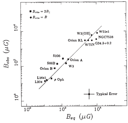
Figure 1.: Observed vs. virial equilibrium values of the magnetic field for the cloud sample of Myers & Goodman 1988a.

Additionally, they also found that $B_{\rm obs}\sim\rho^{1/2}$, in agreement with $\sigma^{2}\sim B^{2}/\rho$ (again derived from combining relations [15] and [16]), since in their sample $\sigma$ had relatively little scatter compared with the other quantities. The resulting correlation had a scatter consistent with the scatter in $\sigma$ (fig. 2).

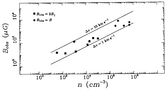
Figure 2.: Observed magnetic field strength vs. virial density $n\equiv 15(32\pi\ln 2mG)^{-1}(\Delta v/R)^{2}$ for the cloud sample of Myers & Goodman 1988a. The solid lines indicate the virial equilibrium model for the indicated velocity dispersions.

Note, however, that in the latter plot, the “virial” density they used was an estimate assuming virial equilibrium ($\rho\propto(\Delta v/R)^{2}$), not an actual observed value, and thus this plot can only be taken as a proof of self-consistency of the virial equilibrium hypothesis.

Myers & Goodman (1988b) also considered the fact that the observed linewidths contain both a thermal and a nonthermal component, explaining deviations from Larson’s (1981) trends at very small scales (cloud cores of sizes $\sim 0.1$ pc). According to relation (13), which refers to the macroscopic, nonthermal velocity dispersion, at small enough cloud sizes the nonthermal component becomes smaller than the thermal (the velocity dispersion becomes subsonic). Indeed, Myers & Goodman (1988b) find a drop in the ratio of nonthermal to gravitational energy ($K_{\rm NT}/W$) in their cloud sample for small cloud sizes. It is important to note, however, that the trend is marginal when the raw data are used, but clearly noticeable only when the assumption of virial equilibrium is introduced (replacing the true gravitational energy obtained from direct measurements of the size and density by the total kinetic (thermal + nonthermal) energy). From this result, Myers & Goodman (1988b) suggest that the uncertainties in $K_{\rm NT}/W$ arise more from uncertainties in the density and size than from uncertainties in velocity dispersion and tempertaure. However, an obvious alternative possibility is that the scatter is real, indicating departures from precise virial equilibrium. Their plot “assuming virial equilibrium” is in reality just a plot of the ratio of nonthermal to total kinetic energy, thus necessarily being very tight at large scales if the velocity dispersion does increase with size while the temperature remains roughly constant, but it is not a test of virial equilibrium in the clouds. On the other hand, further supporting evidence for virial equilibrium has been provided by Goodman et al. (1993), who find good agreement between the observed and the “virial” values of $\beta$, the ratio of rotational to gravitational energy in a sample of dense cores.

The role of thermal plus nonthermal (TNT) motions has been further investigated by Fuller & Myers (1992) and by Caselli & Myers (1995), finding respectively that the scaling of the nonthermal part of the velocity differs from that of the total velocity dispersion, and that the scaling is different for massive cores than for low-mass cores. Furthermore, Fuller & Myers (1992) have distinguished between cloud-to-cloud scaling, i.e., that obtained when the sample consists of various clouds observed with the same tracer (sensitive to one particular density range) and line-to-line scaling, i.e., the scaling obtained when using various tracer molecules (sensitive to a variety of density ranges) on a single cloud. The latter can be used to test for virialization and the density structure of individual clouds as a function of the distance from the core. An even finer subdivision of possibilities has been proposed by Goodman et al. (1997). These authors have additionally found that the slope of the $\sigma$-$R$ relation using single-line, single-cloud measurements, appears to decrease to nearly zero at scales $\sim 0.1$ pc, and that the column density $N$ changes its size dependence from $N\sim R^{-0.2}$ at scales $\lower 2.15277pt\hbox{$\;\buildrel>\over{\sim}\;$}0.1$ pc to $N\sim R^{-0.9}$ at scales $\lower 2.15277pt\hbox{$\;\buildrel<\over{\sim}\;$}0.1$ pc. They interpret these results as evidence for a transition from non-thermal to predominantly thermal support, and the onset of “velocity coherence” at those scales.

Finally, it should be noted that a number of other possible mechanisms, capable of originating Larson’s relations or either one thereof, have been proposed. For example, Larson (1981) himself suggested that the density-size relation might be due to planar shocks which keep the column density constant along the direction of shock propagation. Chièze (1987) has proposed that an ensemble of clouds on the verge of gravitational instability in an environment providing external pressure should also satisfy Larson’s relations. In the chapter on Turbulence in Molecular Clouds, a discussion on mechanisms related to hydro- or magnetohydrodynamic turbulence is given. Other scenarios are unfortunately out of the scope of this course.

3.3. Counterpoint

As it may have started to be apparent to the reader from the discussion of the previous section, the issue of cloud virialization as the origin of the Larson (1981) relations is not completely settled. Besides the caveats inherent to the work of Myers & Goodman (1988a, b), which are the standard references for observational determinations of virial equilibrium in clouds, other somewhat contradictory evidence exists.

First, let us distinguish between a cloud being in virial equilibrium and it satisfying the VT. Actually, all clouds, and in general all fluid parcels in the ISM, satisfy the VT, as it is a direct consequence of the momentum conservation equation. Instead, virial equilibrium means $d^{2}I/dt^{2}=0$ specifically.

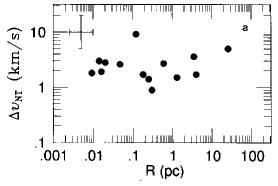
Figure 3.: Nonthermal linewidth vs. size for 14 objects from Myers & Goodman 1988a. No clear correlation is seen. (From Mouschovias & Psaltis 1995.)

Concerning the velocity dispersion-size relation, Scalo (1990) and Mouschovias & Psaltis (1995) have pointed out that the original compiled by Myers & Goodman (1988a) show essentially just scatter for this relation (fig. 3). Mouschovias & Psaltis (1995) “solve the problem” by plotting instead the ratio $\sigma/R^{1/2}$ vs. the magnetic field strength $B$. In reality, however, this is nothing but the same $B_{\rm obs}$ vs. $B_{\rm eq}$ plot shown by Myers & Goodman (1988a). Moreover, Mouschovias & Psaltis (1995) use this result as an argument in favor of the $\sigma$-$R$ relation being a consequence of magnetic support. However, they arrive at this conclusion by assuming $B$ does not “vary much from place to place in the ISM under conditions suitable for the formation of self-gravitating clouds”; yet, the magnetic field strength data they consider vary by three orders of magnitude! In summary, the cloud data discussed in Myers & Goodman (1988a) are consistent with magnetic support, but do not satisfy the dispersion-size relation.

Furthermore, there exists both observational and numerical evidence that the density-size relation is not always satisfied, implying that the column density is not constant. It was already pointed out by Larson (1981) himself that the density-size relation might not be a real property of molecular clouds, but instead just an artifact of limitations of the observational methods used to produce cloud surveys. Kegel (1989) and Scalo (1990) elaborated on this issue. Also, a number of observational studies have found significantly different scaling exponents for both Larson’s relations, or no clear scaling at all. For example, Carr (1987) has found $\sigma\sim R^{0.25}$ and $M\sim R^{2.5}$, implying $\rho\sim R^{-0.5}$ for 45 clumps in the Cep OB 3 molecular cloud. In fact, Carr notes that the clumps are not in virial equilibrium, and concludes that they must be expanding. Loren (1989) studied 89 clumps in the $\rho$ Oph molecular cloud, finding $\rho\sim R^{-0.2}$ and no $\sigma$-$R$ correlation. He points out that many of the clumps are extremely filamentary and that they may probably be the outcome of the passage of a shock wave. Falgarone et al. (1992) focused on low brightness areas of several molecular clouds, including both gravitationally bound and unbound structures (structures for which the actual masses are much smaller than the value obtained assuming virial equilibrium), finding $\sigma\sim R^{0.4}$, and a density-size plot with large scatter and an upper bound given by a Larson-type relation $\rho\sim R^{-1}$. Vázquez-Semadeni et al. (1997) have found the same effect in numerical simulations of turbulent cloud formation in the ISM, in which in fact there is no unique $\rho$-$R$ correlation. Plume et al. (1997), in a sample of maser-selected, massive star formation regions, find no significant $\sigma$-$R$ or $\rho$-$R$ correlations either.

Finally, Myers et al. (1995) have found an example of a cloud in which the kinetic and magnetic energies are comparable, yet the gravitational energy is roughly 500 times smaller, indicating that self-gravity is negligible for this cloud.

4. Discussion and conclusions

From the discussion in the previous sections, a number of points can be concluded.

1. “Virial equilibrium”, i.e., $d^{2}I/dt^{2}=0$ allows up to a constant rate of change in the moment of inertia $I$, even though it is commonly taken to mean a stationary equilibrium.

2. Larson’s (1981) relations, eqs. (13) and (14), have been interpreted as a consequence of virial equilibrium between self-gravity on the one hand and turbulent velocity dispersion and/or magnetic support on the other. From the observational data discussed above, this interpretation may apply to strongly condensed clumps which, due to self-gravity, have decoupled from their surrounding medium, and thus require internal support against collapse.

3. The above interpretation, however, is insufficient for explaining both scaling relations. One is still independent and requires an additional explanation. A critical mass-to-flux ratio has been invoked as the origin of the density-size relation assuming roughly constant magnetic field strengths (Shu et al. 1987; Myers & Goodman 1988b; Mouschovias & Psaltis 1995), but this assumption is not verified in the observational data. For example, the magnetic field strenghts discussed by Myers & Goodman (1988a) and Mouschovias and Pslatis (1995) span three orders of magnitude. Besides, examples of virialized clouds which however follow different scaling relations exist (e.g., Loren 1989; Fuller & Myers 1992; Caselli & Myers 1995; Goodman et al. 1997; see also Vázquez-Semadeni & Gazol 1995 for a theoretical discussion). Planar shocks have also been invoked as an explanation of the apparently constant column densities (Larson 1981; Scalo 1987).

4. It is possible that the density-size relation is not a true property of clouds, but only an observational effect due to the limited integration times used in surveys (Larson 1981; Kegel 1989; Scalo 1990), which tend to select constant-column density obejcts. In this case, surveys using larger integration times would exhibit an increasingly larger scatter in density-size plots, as in the data of Falgarone et al. (1992) or the numerical data of Vázquez-Semadeni et al. (1997), the latter being free from such limitations. In fact, large scatter was already present in the Myers & Goodman (1988b) data. Although they interpreted it as uncertainty in the data rather than real scatter about virialization, the latter possibility is equally feasible. A study that seemed to find exceptionally constant column densities while claiming a large dynamic range (Wood et al. 1994) has been questioned by Vázquez-Semadeni et al. (1997).

5. The velocity dispersion-size relation does not appear subject to the possibility of a spurious origin, and therefore it is probably real when detected, although in many cases it is not (e.g., Loren 1989; Plume et al. 1997). For the cases when it is present, a number of physical mechanisms are plausible candidates. If the density-size relation is not verified, then the standard arguments based on virial equilibrium between gravity and velocity dispersion cannot be invoked (recall the $\sigma$-$R$ relation is a consequence of virial equilibrium and the density-size relation). In particular, the possibility that the $\sigma$-$R$ relation is a consequence of the characteristic energy spectrum of an ensemble of shocks in the flow has been suggested by a number of authors (e.g., Passot et al. 1988; Padoan 1995; Gammie & Ostriker 1996; Fleck 1996; Vázquez-Semadeni et al. 1997). In this case, the origin of the dispersion-size relation would be completely independent of the virial condition, explaining why the relation can be present even in the absence of a density-size relation.

6. In summary, the Larson’s relations and their virial equilibrium interpretation probably apply to relaxed, strongly self-gravitating clumps. Regions which do not exhibit clear scaling relations often include either massive cores (Caselli & Myers 1995; Plume et al. 1997) or regions with strong evidence of recent perturbations (Loren 1989). In fact, the dense cores studied by Plume et al. were selected by the presence of H₂O masers, suggesting strong excitation mechanisms as well. Such “perturbed” regions are likely not in virial equilibrium, thus also being transients (e.g., Magnani et al. 1993), or at least having strongly fluctuating moments of inertia (shapes and internal mass distributions).

Acknowledgments.

The author wishes to thank A. Goodman, T. Passot and J. Scalo for a critical reading of the manuscript, as well as helpful comments and precisions.

References

Ballesteros-Paredes & Vázquez-Semadeni 1997 in preparation

Bally, J., Langer, W. D., Stark, A. A. & Wilson, R. W. 1987, ApJ, 312, L45

Bertoldi, F., & McKee, C. F. 1992, ApJ, 395, 140

Bonazzola, S., Falgarone, E., Heyvaerts, J., Pérault, M., Puget, J. L. 1987, A&A 172, 293

Carr, J. S. 1987, ApJ, 323, 170

Caselli, P. & Myers, P. C. 1995, ApJ, 446, 665

Chandrasekhar, S. 1951, Proc. R. Soc. London, 210, 26

Chièze, J. P. 1987, A& A, 171, 225

Cowling, T. G. 1976, Magnetohydrodynamics (Bristol: Adam Hilger Ltd.)

Currie, I. G., 1974, Fundamental Mechanics of Fluids (New York: McGraw-Hill)

Dame, T., Elmegreen, B. G., Cohen, R., Thaddeus, P. 1986, ApJ, 305, 892

Falgarone, E., & Pérault, M. 1987, in Physical Processes in Interstellar Clouds, ed. G. Morfill, & M. Scholer (dordrecht: Reidel), 59

Falgarone, E., Phillips, T. G., & Walker, C. K. 1991, ApJ, 378, 186

Falgarone, E., Puget, J.-L., & Pérault, M. 1992, A&A, 257, 715

Fleck, R. C. 1996, ApJ, 458, 739

Fuller, G. A., & Myers, P. C. 1992, ApJ, 384, 523

Gammie, C. F. & Ostriker, E. 1996, ApJ, 466, 814

Goodman, A. A., Benson, P. J., Fuller, G. A. & Myers, P. C. 1993, ApJ, 406, 528

Goodman, A. A., Barranco, J. A., Wilner, D. J. & Heyer, M. H. 1997, ApJ, submitted

Jura, M. 1987, in Interstellar Processes, ed. D. J. Hollenbach & H. A. Thronson (Dordrecht: Reidel), 3

Kegel, W. H. 1989, A&A, 225, 517

Landau, L. D. & Lifshitz, E. M. 1987, Fluid Mechanics, 2nd Ed. (Oxford: Pergamon Press)

Larson, R. B. 1981, MNRAS, 194, 809

Léorat, J., Passot, T., & Pouquet, A. 1990, MNRAS, 243, 293

Lesieur, M. 1990, Turbulence in Fluids, $2^{\rm nd}$ ed. (Dordrecht: Kluwer)

Loren, R. B. 1989, ApJ, 338, 902

Magnani, L., LaRosa, T. N., & Shore, S. N. 1993, ApJ, 402, 226

McKee, C. F., Zweibel, E. G. 1992, ApJ, 399, 551 (MZ92)

Mestel, L., & Spitzer, L. 1956, MNRAS, 116, 503

Mestel, L. 1965a, QJRAS, 6, 161

Mestel, L. 1965b, QJRAS, 6, 265

Miesch, M. S., & Bally, J. 1994, ApJ, 429, 645

Mouschovias, T. Ch. 1987, in Physical Processes in Interstellar Clouds, ed. G. E. Morfill & M. Scholer (Dordrecht: Reidel)

Mouschovias, T. Ch. & Spitzer, L., Jr. 1976, ApJ, 210 326

Mouschovias, T. Ch. & Psaltis, D. 1995, ApJ, 444, L105

Myers, P. C., & Goodman, A. A. 1988a, ApJ, 326, L27

Myers, P. C., & Goodman, A. A. 1988b, ApJ, 329, 392

Myers, P. C., & Goodman, A. A. 1991, ApJ, 373, 509

Myers, P. C., Goodman, A. A., Güsten, R. & Heiles, C. 1995, ApJ, 442, 177

Padoan, P. 1995, MNRAS, 277, 377

Passot, T. Vázquez-Semadeni, E., & Pouquet, A. 1995, ApJ, 455, 536

Passot, T., Pouquet, A. & Woodward P., 1988, A&A, 197, 228

Plume, R., Jaffe, D. T., Evans, N. J. II, Martín Pintado, J., & Gómez-González, J. 1997, ApJ, in press

Scalo, J. M. 1987, in Interstellar Processes, ed. D. J. Hollenbach and H. A. Thronson (Dordrecht: Reidel), 349

Scalo, J. M. 1990, in Physical Processes in Fragmentation and Star Formation, ed. R. Capuzzo-Dolcetta, C. Chiosi, & A. di Fazio (Dordrecht: Kluwer), 151

Shore, S. N. 1992, An Introduction to Astrophysical Hydrodynamics (San Diego: Academic Press)

Shu, F. 1992, Gas Dynamics (Mill Valley: University Science Books)

Shu, F., Adams, F. C., Lizano, S. 1987, ARAA, 25, 23

Spitzer, L., Jr., 1978, Physical Processes in the Interstellar Medium (New York: Wiley-Interscience)

Strittmatter, P. A. 1966, MNRAS, 132, 359

Torrelles, J. M., Rodríguez, L. F., Cantó, J., Carral, P., Marcaide, J., Moran, J. M., & Ho, P. T. P. 1983, ApJ, 274, 214

Vázquez-Semadeni, E., Ballesteros-Paredes, J. & Rodríguez, L. F. 1997, ApJ, 474, 292

Vázquez-Semadeni, E. & Gazol, A. 1995, A&A, 303, 204

Vázquez-Semadeni, E., Passot, T. & Pouquet, A. 1995, ApJ, 441, 702

Wood, D. O. S., Myers, P. C., & Daugherty, D. 1994, ApJS, 95, 457

Xie, T. 1997, ApJ, in press

Zweibel, E. G. 1990, 348, 186