Star Cluster Ecology I

Abstract

Star clusters with a high central density contain an ecological network of evolving binaries, affected by interactions with passing stars, while in turn affecting the energy budget of the cluster as a whole by giving off binding energy. This is the first paper in a series aimed at providing the tools for increasingly realistic simulations of these ecological networks.

Here we model the core of a globular star cluster. The two main approximations are: a density of stars constant in space and time, and a purely single star population in which collisions between the evolving stars are modeled. In future papers in this series, we will relax these crude approximations. Here, however, they serve to set the stage before proceeding to the additional complexity of binary star interactions, in paper II, and background dynamical evolution, in later papers.

1 Introduction

In dense stellar systems, such as open and globular clusters and galactic nuclei, encounters between individual stars and binaries can affect the dynamical evolution of the system as a whole on a time scale comparable to, or even shorter than, a Hubble time. In order to reach a detailed theoretical understanding of such systems, the following three steps are necessary.

First, we need to understand the basic mechanism of the dynamical evolution, in the limit of a point-mass approximation for the stars. Second, effects of dynamical encounters on the internal evolution of single stars and binaries has to be taken into account. Third, we have to model the feedback of these internal changes onto the dynamical evolution of the whole system. Let us briefly review each step.

Great progress has been made with the first step, modeling the dynamical evolution of point-mass systems. In the seventies, the processes of core collapse and mass segregation were studied with the use of various types of Fokker-Planck approximations. In the eighties, these simulations were extended successfully beyond core collapse, and various studies were made of the phenomenon of gravothermal oscillations, ubiquitous in the post-collapse phase. Of these models a few even include mass loss due to the evolution of the stars ([Chernoff & Weinberg 1990]). In the nineties, we are finally beginning to switch over from Fokker-Planck approximations to much more detailed and realistic $N$-body simulations. In 1995, the construction of the GRAPE-4, a special-purpose machine with Teraflops speed, has made a $32,000$–body simulation feasible, providing the first direct evidence of gravothermal oscillations (Makino, 1996a,b). Extending these simulations to the full realm of globular clusters ($N=10^{5}\sim 10^{6}$) will require Petaflops speed, something that could be realized by future special-purpose machines in the GRAPE series by as early as the year 2000.

While the point-mass approximation provides a good qualitative guide for the construction of dynamical models of dense stellar systems, this approximation quickly breaks down when we require quantitatively accurate results. The second step attempts to model the effects of close encounters. A number of different investigations have estimated the rate at which physical collisions have take place, under various circumstances ([Hills & Day 1976], [Verbunt & Meylan 1988], [Di Stefano & Rappaport 1992] and [Davies & Benz 1995]). However, little progress has been made so far in following the changes induced in the stellar population, beyond enumerating the number of mergers. In the simulations presented below, collisions are modeled in an evolving population of single stars in a high-density stellar environment. Paper II in this series will extent our treatment to follow the induced changes in binary systems, both on the level of changes in orbital parameters as well as in the internal structure of the stars.

However, such investigations are only a start, and cannot lead to a quantitative modeling of dense stellar systems, since they are not yet self-consistent. What is needed in addition is a treatment of the feedback mechanism, from the changes in single stars and binaries back to the overall dynamics of the system. This third step is being pioneered for open clusters by [Aarseth 1996]. The current series of papers aims to provide self-consistent models of this type, by coupling relatively crude stellar evolution recipes, documented and tested in papers I and II, to a fully dynamical $N$-body system.

This paper is organized as follows. Our approach to the study of the ecology of star clusters is summarized in somewhat more detail in §2. The next section, §3, describes our simulation techniques, and the various approximations involved. In §4, we present the result of a simulation starting a single model, with a minimum of free parameters. The results of a more realistic core model run are presented in §5. §6 sums up.

2 Star Cluster Ecology

Stellar evolution plays a role in star cluster evolution similar to the role played by nuclear physics in stellar evolution. In both cases, the microphysical processes play a crucial role in the mechanism of energy generation in the central parts of the system under consideration, a mechanism that tries to balance the energy losses at the outskirts (tidal radius and photosphere, respectively).

In the next two subsections we look separately at the different forms of physics input necessary to follow the evolution of a star cluster. The third subsection then discusses their interconnection. For future reference, initial conditions are discussed in the fourth subsection, while the last subsection provides a brief outline of the series of papers of which this one is the first.

2.1 Stellar Dynamics Simulations

Great progress has been made in the study of star cluster dynamics, using various approximate methods in which the stars have been treated like a form of fluid, either three-dimensional as in conducting gas sphere models, or six-dimensional as in Fokker-Planck models. In both cases, the main effect of encounters has been taken into account by a form of effective two-body relaxation. We refer to [Hut et al. 1992] for a review of these methods.

Unfortunately, both methods have two intrinsic handicaps that make them unsuitable for a detailed quantitative modeling of the evolution of a globular cluster past core collapse. First, they are not set up to deal with the separate evolution of internal and external degrees of freedom of the binaries that play a central role in the energy generation processes in the cluster.

The second problem stems from an introduction of a mass spectrum, as well as a distinction between stars of different radii, such as dwarfs, main-sequence stars, and giants. The root of the problem here is that a gas sphere or Fokker-Planck approach does not follow individual stars, but rather distribution functions. When the number of independent parameters characterizing the distribution functions becomes too large, there will be less than one star left in a typical cell in parameter space — something that clearly invalidates the statistical hypothesis on which these methods are based.

The only solution is to drop the statistical assumption, and to revert to a star-by-star modeling of a globular cluster, through direct $N$-body calculations. The draw back of such an approach has long been the prohibitive calculational costs involved, and until recently typical production runs only included a few thousand stars. To extend such numbers to include several hundred thousand stars, characteristic of realistic globular clusters, requires an increase of two orders of magnitude in star number, or a factor million in computational cost, from Gigaflops days to Petaflops days ([Hut et al. 1988]).

Recently, the number of stars modeled in direct $N$-body calculations has been increased significantly, to $N=32,000$, using the GRAPE-4, a form of special-purpose hardware developed by a group of astrophysicists at Tokyo University, running at a speed of 1 Tflops (Makino 1996a). The first scientific results of the GRAPE-4, including the first convincing evidence of gravothermal oscillations in $N$-body simulations, predicted by [Sugimoto & Bettwieser 1983], have been presented by Makino (1996ab).

The next, and definitive step that will enable any globular cluster to be modeled realistically might take place as early as the year 2000. If funding can be found, there is no technological obstacle standing in the way of a speedup of the current GRAPE-4 machine by a factor of a thousand, during the next five years. Most of this speed-up will come from further miniaturization, allowing a larger number of gates to be mounted on a single chip, and allowing a higher clock speed as well. A Petaflops machine by the year 2000, allowing simulations of core collapse and post-collapse evolution with up to $10^{6}$ particles, is thus a realistic goal.

2.2 Stellar Evolution Population Synthesis

The first serious attempts to understand and simulate the evolution of close binaries were made in the mid thirties ([Haffner & Heckmann 1937]) and late fifties by [Crawford 1955], [Kopal 1956] and [Huang 1956] followed by [Morton 1960] and the standard work in binary evolution from [Kippenhahn & Weigert 1967]. Synthesis of complete populations of single stars became popular in the mid seventies when [Tinsley & Gunn 1976] simulated the giant-branch luminosity functions for giant elliptical galaxies. However, it is only recently that detailed studies simulate complete populations of close binaries starting with [Dewey & Cordes 1987] who tried to understand the evolutionary sequence of radio pulsars and the presence of an asymmetry in the velocity distribution of single radio pulsars. In later papers, similar evolutionary scenarios for the formation of binary neutron stars were studied in more detail ([Tutukov & Yungelson 1993], [Lipunov et al. 1995], [Portegies Zwart & Spreeuw 1996] and [Lipunov et al. 1996]), for high mass X-ray binaries and the supernova rate in the galaxy ([Tutukov et al. 1992], [Lipunov 1994], [Dalton & Sarazin 1995], [Portegies Zwart & Verbunt 1996]) and for lower mass systems with a neutron star ([Webbink & Kalogera 1993], [Pols & Marinus 1994]) or a white dwarf ([de Kool 1990], [Kolb & Ritter 1992]) as the accreting object. The first couragous attempt to combine stellar and binary evolution within the collisional evironment of a globular cluster was performed by [Sutantyo 1975], followed more recently by [Di Stefano & Rappaport 1992], [Sigurdsson & Phinney 1993], [Leonard 1994], [Davies & Benz 1995] and [Davies 1995].

2.3 Ecological Networks

Purely stellar-dynamical calculations often rely on rather severe approximations, such as a representation of stars by equal-mass point-masses. And there is a good reason for doing so, since any single deviation from that simple recipe requires other deviations as well. Let us look at one example.

As soon as we introduce a mass spectrum in a star cluster simulation, we will see that the heavier stars start sinking toward the center, on the dynamical friction time scale, shorter than the two-body relaxation time by a factor proportional to the mass ratio of individual heavy stars with respect to that of typical stellar masses. The reason is that relaxation tends toward equipartition of energy, which implies that heavier stars will move more slowly and therefore gather at the bottom of the cluster potential well.

If stars would live forever, there would be a large overconcentration of heavy stars in the core of a star cluster. However, in reality there is an important counter-effect: heavy stars burn up much faster than lighter ones. They may or may not leave degenerate remnants, that may or may not be heavier than the average stellar mass in the cluster (a quantity that decreases in time). Clearly, it would be grossly unrealistic to introduce a mass spectrum without removing most of the mass of the heaviest stars on the time scale of their evolution off the main sequence and across the giant branches.

Another reason for introducing finite life times for stars comes from abandoning the very restrictive point mass model. As soon as we do that, giving our stars a finite radius will give rise to stellar collisions. The heavier stars produced in the collision of two turn-off stars, for example, will burn up on a time scale an order of magnitude smaller than the age of the cluster. Again, we have to take this into account to be consistent, especially since the merger products themselves are prime candidates for further merging collisions.

The need to let many stars shed most of their mass, together with the fact that most of the energy in a globular cluster is locked up in binaries, poses a formidable consistency problem. Since binaries play a central role in cluster dynamics, consistency requires that we follow their complex stellar evolution, which involves mass overflow (which can be stable or unstable, and can take place on dynamical or thermal or nuclear time scales) and the possibility of a phase of common-envelope evolution. On top of all that, we will have to find simple recipes for the hydrodynamic effects occurring in three-body and four-body reactions, and in occasional $N>4$ reactions, which are bound to occur in dense cluster centers.

To sum up: there does not seem to be a half-way stopping point, at which we can expect to carry out consistent cluster evolution simulations. Either we study the interesting but unrealistic mathematical-physics problem of an equal-mass point particle model, or we opt for a realistic model with some set of stellar-evolution recipes. The main question here is: what is the simplest set that is still consistent?

2.4 Initial Conditions

In most stellar dynamics simulations of star clusters, the Plummer model is used as a standard model to specify the initial conditions for the distribution of the point particles. While not very realistic, this choice has had the advantage of making comparisons between different runs, as well as between different approaches, relatively straightforward. Of course, when attempts are made to model particular star clusters, other models have often replaced the Plummer model as a starting point. King models, for example, are already more realistic in that they provide a form of spatial cut-off that can be interpreted as a tidal radius.

For similar reasons, we will use a standard model for our simulations that combine stellar dynamics and stellar evolution. In most cases, the use of our standard model will be mostly for illustrative reasons, to provide a gauge for comparison between our various results, as well as between our results and that of others. For historical reasons, we choose our standard model to be based on a Plummer model for the macroscopic initial star distribution, and a Salpeter model for the initial mass function.

An additional advantage of these simple choices is that they limit the number of free parameters. The Plummer model, for example, contains only one free parameter, $N$, the number of stars in the system (apart from a choice of mass and length scales, that are irrelevant in the point particle case). In contrast to the Plummer model, our standard model can be expected to form a multi-parameter family. As soon as we abandon the point-mass approach, we have to deal with microscopic as well as macroscopic mass and length scales.

Of these various scales, the macroscopic quantities can be chosen independently, while the microscopic ones can be fixed, statistically, by specifying a mass distribution together with appropriate cut-off masses at the high and low end. In general, an arbitrary functional form for the mass distribution function can lead to an arbitrarily large number of parameters. Interestingly, our standard model definition allows us to limit the total number of free parameters to three.

Starting from the macroscopic side, we can take the total mass $M$ and the half-mass radius $r_{h}$ of the Plummer model as our first two free parameters. With a Salpeter choice of powerlaw distribution function, the third free parameter can be chosen in the form of the lower mass cut-off $m_{-}$. The higher-mass cut-off $m_{+}$ could be specified independently, but this is not strictly necessary: since the Salpeter distribution function converges at the high-mass end, we can simply parcel out the total mass $M$ over different stellar masses, between star masses of $m=m_{-}$ and $m_{+}=\infty$, and we will naturally be left with a single most massive star. This procedure is not unrealistic: nature probably limits the number of high-mass stars in medium-size galactic clusters in a similar way.

In fact, we can go even further, and make the following somewhat arbitrary but natural choices: $r_{h}=10$ pc, $m_{-}=0.1\mbox{${\rm M}_{\odot}$}$. This leaves only the total mass $M$ to be specified, or equivalently, the total number of stars $N$. For future convenience, we will refer to this ‘most standard’ model as our reference model. For systems with a few thousand stars, we are dealing with a typical open cluster, with velocity dispersions of order 1 km/s, while for a few hundred thousand stars, we have a reasonable approximation to a globular cluster, for which typical stellar velocities are an order of magnitude higher.

In addition to this standard model, the various papers in this series will also contain the results of more realistic models. However, we will typically provide at least one run from a standard model, in order to provide comparison material for the more detailed models.

2.5 Stepping Stones

In the current series of papers, our goal is to provide a series of ecological simulations, based on a flexible stellar dynamics code coupled to a comprehensive set of stellar evolution modules. These modules in turn are based on recipes that govern the behavior of both single star and binary star evolution, as well as interactions between larger numbers of stars.

In order to present results that can be reproduced and critically assessed by other groups, we clearly document the recipes used, as well as their coupling to the dynamics. With this aim, we give a detailed description of our approach in the first few papers in this series, which will form stepping stones towards a full-fledged ecological star cluster evolution code.

The present paper starts off with rather extreme approximations for the stellar dynamics, as well as the stellar evolution parts of our simulations. With respect to the former, we start with a laboratory-type situation, in which we consider a homogeneous distribution of stars, kept constant in time. With respect to the latter, we consider a population of single stars only. Paper II will relax the second assumption, by introducing a population of primordial binaries, and allowing the formation of new binaries as well. Later papers will subsequently relax the former assumption, with the ultimate goal of using a self-consistent $N$-body code.

3 A Static Homogeneous Environment with Single Stars

3.1 Initial Conditions

In the present paper, we keep the dynamical environment as simple as possible, in order to focus on the stellar evolution recipes, that are introduced here and used in subsequent papers as well. The stellar distribution is take to be in thermal equilibrium, with a density that is constant in space and time. In addition, an additional simplification is obtained by excluding any primordial binaries, and ignoring binary formation channels. Within this setting, random encounters between single stars will lead to collisions resulting in the formation of merger products, the evolution of which can then be followed along with the evolution of the original single stars.

3.1.1 Initial Mass Function

While our main aim is to set-up and clarify our stellar evolution recipes, we present two calculations that could be interpreted as having a limited astrophysical interpretation, one for the core of an $\omega$-Centauri-like cluster (§4), and one for the core of an M-15-like cluster (§5). Our choice of constant density implies that we can only hope to model the history of a cluster core, not that of a cluster as a whole. To specify the mass distribution, we first take our standard choice: a Salpeter initial mass function (§4), which we will use to model a relatively unevolved core. Our second choice will be a much more flat distribution, which is more appropriate for a high-density post-collapse cluster core (§5).

3.1.2 Mass and Number Densities

If we specify the mass density $\rho$ for the stars in our cluster case, we can use the mass function to determine the number density $n=n(\rho)$. In a homogeneous medium the relation is linear, and for the simplest case of a powerlaw mass function $f(m)\propto m^{-\alpha}$, we find

$${n\over\rho}={{\alpha-2}\over{\alpha-1}}{{m_{-}^{1-\alpha}-m_{+}^{1-\alpha}}\over{m_{-}^{2-\alpha}-m_{+}^{2-\alpha}}},$$ (1)

where $m_{-}$ and $m_{+}$ are the lower and upper mass cut-offs, respectively. For the example of an initial Salpeter mass function, $\alpha=2.35$, we find

$${n\over\rho}={0.26\over m_{-}},$$ (2)

when we neglect the fact that the upper mass cut-off is finite. The inverse quantity $m_{av}$ is the average stellar mass:

$${m_{av}}={3.9m_{-}}=0.39\mbox{${\rm M}_{\odot}$}$$ (3)

in our standard case where we take a lower cut-off mass of $0.1\mbox{${\rm M}_{\odot}$}$. The median mass $m_{med}$ for a Salpeter distribution is

$${m_{med}}=2^{1\over{\alpha-1}}m_{-}=0.17\mbox{${\rm M}_{\odot}$}$$ (4)

which means that in our standard population most stars have a mass well below $0.2\mbox{${\rm M}_{\odot}$}$.

Even in our simple case of a homogeneous system, the linear relationship $n(\rho)/\rho=1/m_{av}$ involves a complicated time dependent factor $m_{av}$. Not only does the upper mass cut-off $m_{+}$ (roughly the main sequence turn-off mass) depend on time, but what is worse, the distribution of remnants, in the form of black holes, neutron stars and white dwarfs, does not obey any simple power law, even if their progenitors did. In general, therefore, the coefficient $n/\rho$ has to be determined numerically, as a function of time.

3.1.3 Velocity Dispersions

In thermal equilibrium, equipartition of kinetic energy tells us how the velocity dispersions scale for stars with different masses. We only have to specify the three-dimensional velocity dispersion $v$ for one particular mass, say $v(1\mbox{${\rm M}_{\odot}$})=\mbox{${\rm v}_{\odot}$}$, in order to determine the 3D velocity dispersion $v(m)$ for stars of general mass $m$:

$$v(m)=\left({1\mbox{${\rm M}_{\odot}$}\over m}\right)^{1/2}\mbox{${\rm v}_{\odot}$}.$$ (5)

3.1.4 Core Radius and Core Mass

The three choices discussed so far, namely that of an initial mass function, a density, and a temperature, specify the intensive thermodynamic properties. This in turn enables us to calculate the local rate of collisions, per unit time, and per unit volume. In order to extract global information, we have to specify extensive quantities as well, such as the total volume or total mass of our system. This will allow us to determine a global collision rate per unit time, which we can then compare with that of an astrophysical system, such as the core of a globular cluster.

For an equal-mass cluster model that is close to thermodynamic equilibrium, the density drops by roughly a factor three, from the center to the edge of the core. This implies that the local density of collisions, which is proportional to the square of the density, drops by an order of magnitude. In the more realistic case of a mass spectrum the situation is even worse, since the density of the heavier stars drops off faster than that of the lightest stars. In the present paper we will not attempt to model these density dependent effects, and instead we will keep the density of all mass groups constant throughout the region of our simulation. It is clear, therefore, that our results are mainly for the purpose of illustration, and that any comparison with actual systems will have to be taken with many grains of salt.

The only question remaining is the definition of a core radius $r_{c}$. For an equal mass system, we have ([Spitzer 1987])

$$r_{c}=\left({3\over 4\pi G\rho}\right)^{1/2}v_{c}.$$ (6)

In the presence of a mass spectrum, we have to modify this equation. Although the velocity dispersion is now quite different for different mass groups, the average kinetic energy per star $(1/N)E_{kin}$ is independent of mass, with $N$ the total number of stars in the core. Rewriting the above formula, we have:

$$r_{c}^{2}={3\over 4\pi G\rho}{2\over M}E_{kin},$$ (7)

where $M$ is the core mass. For a general mass spectrum, we can substitute $E_{kin}=(N/2)\mbox{${\rm M}_{\odot}$}\mbox{${\rm v}_{\odot}$}^{2}$ which gives

$$r_{c}=\left({3\over 4\pi G\rho}\right)^{1/2}\left({\mbox{${\rm M}_{\odot}$}\over m_{av}}\right)^{1/2}\mbox{${\rm v}_{\odot}$}.$$ (8)

In this expression, the right hand side contains only local quantities, and the global quantity $r_{c}$ is given in terms of those.

Note that this is not the only possible generalization of the equal-mass expression, but it is a natural one, and it reverts to the original expression in cases where the mass of the core is dominated by stars in a relatively small mass range, as is the case, for example, in a post-collapse core of a globular cluster.

Other global quantities can be derived from $r_{c}$, such as the core mass $M$:

$$M={2\over 3}\pi r_{c}^{3}\rho,$$ (9)

where we have used the fact that in an isothermal sphere the average density in the core is roughly half the central density, a relationship, while not exact, is certainly good enough for our purpose of relating our results to astrophysical systems.

3.2 Recipes for Stellar Evolution

The stars in our computations are evolving. To describe their evolution, we use the formulae fitted to the results of full stellar evolution calculations, by [Eggleton et al. 1989]. These formulae give the radius and luminosity (for population I stars) as a function of time, on the main sequence, in the Hertzsprung gap, the (sub)giant branch, on the horizontal branch, and on the asymptotic giant-branch. We use these population I recipes, because the more appropriate data for population II stars are not available in the same convenient form. In addition to the radius, we need the core mass for stars that have left the main sequence. We derive these from the luminosity, according to [Eggleton et al. 1989], and core-mass luminosity relations, according to [Boothroyd & Sackmann 1988], [Paczyński 1970] and [Iben & Truran 1978]. The details of this procedure are described in Portegies Zwart and Verbunt (1996, Section 2.1).

3.3 Recipes for Individual Encounters

In this paper, we only treat single stars, and accordingly the only outcome allowed for a close encounter is a merged object. The merging between the two stars in an encounter in our calculation is generally assumed to conserve mass, which in fact may be a reasonable approximation (Benz and Hills 1987, 1989, 1992, Rasio and Shapiro 1991, 1992).

Only a limited number of simulations of encounters between stars has been performed, and these does not cover all possible combinations that may occur in a cluster. Also, different authors do not agree on the details of the outcomes for the same type of encounter. We therefore have chosen to use a set of simple prescriptions for the outcome of stellar collisions, often chosen without detailed justification. In the future these prescriptions can be refined, when more accurate calculations for collisions become available. Meanwhile, our results will help in determining which of all possible types of encounter are most frequent, and therefore deserve closer attention.

Table 1: Simplified representation of possible merger outcomes. The four columns correspond to the four choices given for the type of massive star (primary), while the four rows indicate the type of less massive star (secondary): main-sequence star (ms), (sub)giant (sg), white dwarf (wd) and neutron star (ns). In this table we do not discriminate between stars in the Hertzsprung gap (Hg) or on the first and second ascent on the asymptotic-giant branch (AGB).

	primary
star	ms	sg	wd	ns
			wd	ns
ms	ms	sg	+	+
			disc	disc
			wd	ns
sg	Hg	AGB	+	+
			disc	disc
wd	sg	AGB	–	–
ns	$\mbox{T}\dot{\mbox{Z}}$O	$\mbox{T}\dot{\mbox{Z}}$O	–	–

We describe our treatment of the possible outcomes of the encounters of two stars ordered by the evolutionary state of the more massive of the two, the primary. Table 1 summarizes this treatment.

3.3.1 Main-sequence primary

If both stars involved in the encounter are main-sequence stars the less massive star is accreted conservatively onto the most massive star. The resulting star is a rejuvenated main-sequence star (see Lai et al. 1993, Lombardi et al. 1995). The details of this procedure are described in Appendix C4 of Portegies Zwart and Verbunt (1996).

If the less massive star in the encounter has a well developed core (giant or subgiant) this core is treated as the core of the merger product. The main-sequence star and the envelope of the giant are added together to form the new envelope of the merger. In general the mass of the core is relatively small compared to its envelope and the star is assumed to continue its evolution through the Hertzsprung gap. Note that this type of encounter can only occur when the main-sequence star is in itself a collision product (e.g. a blue straggler).

When a main-sequence star encounters a less massive white dwarf, we assume that the merger product is a giant, whose core and envelope have the masses of the white dwarf and the main-sequence star, respectively. We then determine the evolutionary state of the merger product, as follows. We calculate the total time $t_{\rm agb}$ that a single, unperturbed star with a mass equal to that of the merged star spends on the asymptotic giant-branch, and the mass $m_{\rm c,agb}$ of its core at the tip of the giant branch. The age of the merger product is then calculated by adding $t_{\rm agb}m_{c}/m_{\rm c,agb}$ to the age of an unperturbed star with the same mass at the bottom of the asymptotic giant branch. For example, a single, unperturbed 1.4${\rm M}_{\odot}$ star leaves the main-sequence after 2.52 Gyr, spends 60 Myr in the Hertzsprung gap, moves to the horizontal branch at $2.96\,$Gyr, and reaches the tip of the asymptotic giant branch after $3.06\,$Gyr, with a core of $0.64\,\mbox{${\rm M}_{\odot}$}$. Thus, if a 0.6 ${\rm M}_{\odot}$ white dwarf mergers with an $0.8\,\mbox{${\rm M}_{\odot}$}$ main-sequence star, the merger product has an age of 2.87 Gyr, leaving it another 180 Myr before it reaches the tip of the asymptotic giant-branch.

If the less massive star is a neutron star a Thorne $\dot{\mbox{Z}}$ytkow object ([Thorne & $\dot{\mbox{Z}}$ytkow 1977]) is formed.

3.3.2 Evolved primary

When a (sub)giant or asymptotic branch giant encounters a less massive main-sequence star, the main-sequence star is added to the envelope of the giant, which stays in the same evolutionary state, i.e. remains a (sub)giant, c.q. asymptotic branch giant. Its age within that state is changed, however, according to the rejuvenation calculation described in Section C.3 of Portegies Zwart and Verbunt (1996). For example, an encounter of a giant of $0.95\,\mbox{${\rm M}_{\odot}$}$ and age $11.34\,$Gyr with a 0.45 ${\rm M}_{\odot}$ main-sequence star produces a giant of 1.4 ${\rm M}_{\odot}$ with an age of $2.67\,$Gyr.

When both stars are (sub)giants the two cores are added together and form the core of the merger product (see also the results of the smoothed particle hydrodynamics computations performed by Davies et al. 1991 and Rasio and Shapiro 1995). Half the envelope mass of the (less massive) encountering star is accreted onto the primary. The merger product continues its evolution starting at the next evolutionary state; thus a (sub)giant continues its evolution on the horizontal branch and a horizontal branch star becomes a asymptotic-giant branch star. The reasoning behind this assumption is that an increased core mass corresponds to a later evolutionary stage.

If the less massive star is a white dwarf then its mass is simply added to the core mass of the giant, and the envelope is retained. If the age of the giant before the encounter exceeds the total life time of a single unperturbed star with the mass of the merger, then the newly formed giant immediately sheds its envelope, and its core turns into a single white dwarf; if not then the merged giant is assumed to have the same age (in years) as the giant before the collision, and continues its evolution as a single unperturbed star.

If the encountering star is a less massive neutron-star a Thorne $\dot{\mbox{Z}}$ytkow object is formed.

3.3.3 White-dwarf primary

In an encounter between a white dwarf and a less massive main-sequence star, the latter is completely disrupted and forms a disk around the white dwarf ([Ruffert & Müller 1990], [Rasio & Shapiro 1991]). The white dwarf accretes from this disk at a rate of one percent of the Eddington limit. If the mass in the disc exceeds 5% of the mass of the white dwarf, the excess mass is expelled from the disc at a rate equal to the Eddington limit.

If a white dwarf encounters a less massive (sub)giant, a new white dwarf is formed with a mass equal to the sum of the pre-encounter core of the (sub)giant and the white-dwarf. The newly formed white dwarf is surrounded by a disk formed from half the envelope of the (sub)giant before the encounter. If the mass of the white dwarf surpasses the Chandrasekhar limit, it is destroyed, without leaving a remnant ([Nomoto & Kondo 1991] and [Livio & Truran 1985]).

Collisions between white dwarfs are ignored.

3.3.4 Neutron-star or black-hole primary

All encounters with a neutron star or black hole primary lead to the formation of a massive disk around the compact star. If the compact star had a disk prior to the collision, this disk is expelled. This disk accretes onto the compact star at a rate of 5% of the Eddington limit. An accreting neutron star turns into a millisecond radio-pulsar, or – when its mass exceeds $2\mbox{${\rm M}_{\odot}$}$ – into a black hole. Mutual encounters between neutron stars and black holes are ignored, as are collisions between these stars and white dwarfs.

3.4 Monte Carlo Simulations of Ensembles of Encounters

Each star in our model can encounter any of the other stars. To reduce computational cost, we bin the stars in intervals of mass and radius, and compute the probability for encounters between bins, giving all stars in one bin the same mass and radius, and, through Eq. 2, choosing their velocities from the same distribution. The cross section $\sigma_{ij}$ for a encounter with a distance of closest approach within $d$ between a star from bin $i$ and a star from bin $j$ contains a geometrical and a gravitational focusing contribution:

$$\sigma_{ij}=\pi d^{2}\left(1+2G\frac{m_{i}+m_{j}}{v_{ij}^{2}d}\right),$$ (10)

where $v_{ij}$ is the relative velocity between the stars at infinity. For the minimum separation between the two stars that leads to a collision $d=2(r_{i}+r_{j})$ is used. (The exact distance at which the transition between merger and binary formation occurs is not known –[Kochanek 1992], [Lai et al. 1993]–, we choose the factor 2 arbitrarily.)

In the present paper, we model the stellar distributions as being spatially homogeneous. In order to make contact with astrophysical applications, we will consider our stars to be contained within in a fixed sphere with radius $r_{c}$. While we can consider this radius to stand for the notion of ‘core radius’ in a post-collapse cluster, we want to point out that this interpretation is only an approximate one. In realistic star clusters, there is a significant drop in density across the core, from the center to the core radius. For most stars the density drops by roughly a factor of three, but for the heavier stars, such as neutron stars and especially black holes, this factor can be much larger.

The encounter rate $\Gamma_{ij}$ of stars from bin $i$ with stars from bin $j$, anywhere in the volume of the sphere with radius $r_{c}$ is given by two separate equations:

$$\Gamma_{ij}=\left\{\begin{array}[]{crr}{1\over 2}n_{i}(n_{j}-1)&\langle\sigma_{ij}v_{ij}\rangle{4\over 3}\pi r_{c}^{3}&\,\mbox{for $i=j$}\\ n_{i}n_{j}&\langle\sigma_{ij}v_{ij}\rangle{4\over 3}\pi r_{c}^{3}&\,\mbox{$i<j$},\end{array}\right.$$ (11)

where $n_{i}$ and $n_{j}$ are the number densities of stars in bins $i$ and $j$, respectively, and where $\langle\,\rangle$ indicates averaging over the the distribution of relative velocities $v_{ij}$ (Note that we should have written the last equation with an extra factor $1/2$, if we would have summed over all combinations $i\neq j$, in order to avoid double-counting of collisions).

Since the stars in bins $i,j$ have Maxwellian velocity distributions with root-mean-square velocity $v_{i}$ and $v_{j}$, given by Eq.(2), the relative velocities $v_{ij}$ also have a Maxwellian distribution, with a root-mean-square velocity given by $\sqrt{{v_{i}}^{2}+{v_{j}}^{2}}$. Hence

$$\langle\sigma_{ij}v_{ij}\rangle = \frac{4l^{3}}{\sqrt{\pi}}\int_{0}^{\infty}v_{ij}^{3}\sigma_{ij}\exp(-l^{2}v_{ij}^{2})dv_{ij}$$ (12)

$$= {2\pi d^{2}\over l\sqrt{\pi}}\left(1+2G{m_{i}+m_{j}\over d}l^{2}\right),$$

where we have defined

$$l^{2}={3\over 2({v_{i}}^{2}+{v_{j}}^{2})}.$$ (13)

With this result, we write the encounter rates $\Gamma_{ij}$ in convenient units:

$$\Gamma_{ij} = \frac{n_{i}}{10^{3}\mbox{pc}^{-3}}\frac{n_{j}}{10^{3}\mbox{pc}^{-3}}\left(\frac{r_{\rm c}}{\mbox{pc}}\right)^{3}$$ (14)

$$\times [3.61\cdot 10^{-3}\left(\frac{m_{i}+m_{j}}{\mbox{${\rm M}_{\odot}$}}\right)\left(\frac{r_{ij}}{\mbox{${\rm R}_{\odot}$}}\right)\left(\frac{\mbox{${\rm km~{}s}^{-1}$}}{v_{ij}}\right)$$

$$+ 6.31\cdot 10^{-9}\left(\frac{r_{ij}}{\mbox{${\rm R}_{\odot}$}}\right)^{2}\left(\frac{\mbox{${\rm km~{}s}^{-1}$}}{v_{ij}}\right)^{-1}]$$

$$\,[\mbox{Myr}^{-1}].$$

The total encounter-rate follows as

$$\Gamma=\sum_{ij=1}^{N}\Gamma_{ij}\equiv{1\over\tau_{\rm enc}},$$ (15)

where $N$ gives the total number of bins in mass and radius and $\tau_{\rm enc}$ is the average time interval between two encounters.

The stellar population in our calculation changes both due to encounters between stars, and due to evolution of the stars. The shortest evolutionary time-scale of importance to us is the time scale on which the evolving stars expand; the fastest evolving star in the sample is used to set the evolution time scale

$$\tau_{\rm ev}\equiv\min(R/{\dot{R}}),$$ (16)

where $R$ and $\dot{R}$ are the stellar radius and its time derivative, respectively.

At the beginning of each time step, we distribute the stars over the bins in radius and mass, calculate the number densities of stars in each bin, and the evolution and collision time scales $\tau_{\rm ev}$ and $\tau_{\rm enc}$. The sum over all bins $ij$ is less daunting as may appear at first sight, as many bins contain no stars. This is illustrated in Figure 3. The time step to be taken is then calculated as

$$dt=\min(0.2\tau_{\rm enc},\tau_{\rm ev}),$$ (17)

to ensure that changes in the stellar population are followed with sufficient resolution.

At this point, a rejection technique is used to keep track of collisions, as follows. We choose a random number between 0 and 1. If this number is larger than $\Gamma dt$, we conclude that no collision has occurred. We evolve all stars over a time $dt$, and continue with the next step.

If the random number is smaller than $\Gamma dt$, a collision has occurred. In calculating the sum (Eq. 15) over the bins, we keep track of the partial sum after addition of each bin combination $ij$. The first bin combination for which this growing partial sum exceeds the random number identifies the bins involved in the collision. We then assign a sequence number to each star in bin $i$, and select one of these numbers randomly; and repeat this for bin $j$. If $i$ and $j$ are identical, care is taken that the same star is not selected twice. From the prescriptions in the previous section, we decide the outcome of the collision between the two selected stars.

We then select another random number between 0 and 1, to see whether a second collision has occurred. If so, we determine its outcome. This procedure is repeated until a random number larger than $\Gamma dt$ is found, which indicates that no further encounter has occurred in the time step under consideration.

After each time step $dt$ a number of stars equal to the number of encounters that have taken place is lost from the stellar system; these stars have merged into single objects. For each lost star a new star is added to the computation, in order to guarantee a constant number of stars. The mass of this ‘halo guest’ is determined by the present-day mass-function of the cluster.

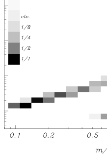
Figure 1: Relative encounter probabilities in model calculation $S$, at time $t=12\,$Gyr, when the turnoff mass is $M_{\rm to}=0.91\,\mbox{${\rm M}_{\odot}$}$, for a single star with $1\mbox{${\rm M}_{\odot}$}$ and $1\mbox{${\rm R}_{\odot}$}$ as a function of mass and radius of the other star involved in the encounter. Darker shades indicate higher probabilities. The compact stars (nominally with zero radius) are shown as a bar below 0.1 ${\rm R}_{\odot}$: neutron stars between 1.34 and 2 ${\rm M}_{\odot}$ and white dwarfs at lower masses. All other stars with radius in excess of the radius at the turnoff are the evolved stars. The masses of these stars is similar to the turnoff mass. A small fraction of blue stragglers is visible as an extension of the main-sequence (to the right of the turnoff). The vertical bar in the upper left corner presents a scaling to the gray shades. The lowest square corresponds to an encounter rate of once every 12.7 Tyr decreasing with a factor of two for each subsequent square. The integrated encounter frequency of the $1\mbox{${\rm M}_{\odot}$},1\mbox{${\rm R}_{\odot}$}$ star is 1 encounter every 1.68 Tyr. Almost 13% of the encounters occur with a main-sequence star with a mass of about $\sim 0.13\mbox{${\rm M}_{\odot}$}$ (black squares below and to the left).

4 A Dynamically Evolving Salpeter Mass Function

Figure 2: Relative frequencies of various types of encounters (upper panel, the curly brackets indicate the collision) and their outcomes (lower panel), for model computation $S$, integrated over the duration of the calculation. Abbreviations: ms main-sequence star, gs giant, wd white dwarf, ns neutron star, Bss blue straggler, Yss yellow straggler.

A total of two models are computed, one with a Salpeter type mass function which we call model $S$ (from Salpeter), and one model which we call model $C$ (from Collapsed) with a mass function that is affected strongly by mass segregation.

In the volume of the stellar system in model $S$, we sprinkle stars according to a Salpeter mass distribution between 0.1${\rm M}_{\odot}$and 100${\rm M}_{\odot}$. The total number of stars is irrelevant, since we are considering these stars to be contained in a laboratory-type enclosure, with a thermal distribution of stellar velocities. Our choice for the ‘temperature’ of this distribution is fixed by requiring that stars with a mass $m=1\mbox{${\rm M}_{\odot}$}$ will have a one-dimensional velocity dispersion of 10.0 km/s, in conformity with the same choice made in §5. The radius of the core was chosen to be $r_{c}=4$ pc and the computation is started at $t=0$ and terminated at an age of 16 Gyr. For the computation of the encounter rate a total of 30 bins in mass, equally spaced in the logarithm of the mass between 0.1 and 100 ${\rm M}_{\odot}$, and 30 bins in radius, equally spaced in the logarithm of radius between 0.1 and 2000 ${\rm R}_{\odot}$ are used. An additional bin with zero radius is used for the compact stars, i.e. the white dwarfs, neutron stars and black holes.

Table 2: Parameters of the different model computations, and corresponding characteristics. Subsequent columns give the name of the model, indication whether a Salpeter mass function or a mass function that is affected by mass segregation is used, core radius, 3-dimensional velocity dispersion ${\rm v}_{\odot}$ time at which encounters are started, the age of the population at the start of the dynamical interactions, the central stellar number-density in the core, the ratio of the number of stars in the computation to the actual number of stars in the core, the number of encounters during the calculation per star, and the average time between two encounters, anywhere in the core.

Model	mf	$r_{\rm c}$	${\rm v}_{\odot}$	$t_{\rm cc}$	$\log n_{c}$	$f_{\rm c}$	$n_{\rm enc}$	$\tau_{\rm enc}$
		[pc]	[km/s]	[Gyr]	[$\star$ pc-3]		$\star^{-1}$	[Myr]
$S$	Salpeter	4.0	17.3	0	3.93	0.298	0.002	5.17
$C$	Segregated	0.1	17.3	10	6.64	8.750	0.660	1.28

Figure 1 shows for model computation $S$, the relative probabilities of encounters with various types of stars for a $1\mbox{${\rm M}_{\odot}$},1\mbox{${\rm R}_{\odot}$}$ star, at an age of the cluster of 12 Gyr. Due to the small encounter frequency hardly any collision products are present in the stellar system. Only a small number of blue stragglers (stars with a mass larger than the turnoff and with similar radii) have finite probability to be involved in an encounter. The most probable partners for an encounter with a $1\mbox{${\rm M}_{\odot}$},1\mbox{${\rm R}_{\odot}$}$ star are the stars at the low end of the main sequence.

In Figure 2 we show the relative frequencies of encounters of different types, and of the resulting collision products for model $S$. Because the steep mass function the collisions rate is dominated by main-sequence stars; the fraction of collisions involving giants is only small. The most frequent type of encounter is one involving two main-sequence stars, leading to a main-sequence merger remnant with a mass smaller than the turnoff mass or a blue straggler when the mass of the merger exceeds the turnoff mass. If the mass of the merger is less than the turnoff mass, the product is a main-sequence star which is younger than primordial main-sequence stars with the same mass. Such a star will be left behind as a blue straggler once the primordial main-sequence stars leave the main-sequence. Yellow stragglers, i.e. giants not on the main (sub)giant branch of the cluster (which approximately coincides with the evolutionary track of a star with the turn off mass), can be formed directly from encounters between a main-sequence star and a giant, between a main-sequence star and a white dwarf and between a giant and a white dwarf, in decreasing order of importance; encounters between two giants are extremely rare. Our prescriptions put every merger product on the evolutionary track of an ordinary star; the presence of yellow stragglers in our calculations is therefore only due to the formation of giants with a mass larger than the turnoff mass.

5 A More Realistic Mass Function

The initial conditions for the mass function of the computation of model $C$ (for collapsed cluster core) are chosen to be more realistic, in the sense that the mass function is flattened due to mass segregation in the previous evolution of the stellar system. The lack of detailed computations concerning the present-day mass function in the cores of globular clusters, justifies our choice to use a mass function similar to the one described by [Verbunt & Meylan 1988]. For the mass function of model $C$ we consider three classes of objects: non-degenerate stars (main-sequence stars and giants), white dwarfs, and neutron stars. The more massive stars have all evolved, and left inert remnants (white dwarfs or neutron stars). We assign a certain fraction of the total number of stars in the stellar system to each of these classes. All neutron stars (5% of the total number of stars) are assumed to have the same mass (of $1.34\mbox{${\rm M}_{\odot}$}$). The mass distribution within the two other classes are described with power-laws with a slope of $\alpha=0$ for the main-sequence stars and the (sub)giants and a slope of $\alpha=1$ for the white dwarf progenitors. At the start of the dynamical modeling a total number fraction of main-sequence stars and giants of 70% is chosen, this number decreases as the stellar system evolves. The minimum initial mass of a main-sequence star is chosen to be 0.2${\rm M}_{\odot}$ instead of the 0.1${\rm M}_{\odot}$ for models $S$.

The numbers of stars in the different classes change as time evolves due to stellar evolution, encounters between stars, and due to the addition of a star, each time that the number of stars has decreased by one in a merger process.

Figure 3: Relative encounter probabilities in model calculation $C$, at time $t=12\,$Gyr, when the turnoff mass is $M_{\rm to}=0.91\,\mbox{${\rm M}_{\odot}$}$, for a single star with $1\mbox{${\rm M}_{\odot}$}$ and $1\mbox{${\rm R}_{\odot}$}$ as a function of mass and radius of the other star involved in the encounter (similar to Fig. 3). The high encounter-rate and different mass function result in an enormous enrichment of collision products in the stellar system. Besides the small fraction of black holes (nominally with zero radius an with a mass larger than 2${\rm M}_{\odot}$), there is also a rich population of blue stragglers (in the area with a mass larger than the turn off and a radius larger than about one ${\rm R}_{\odot}$) and yellow stragglers (stars with a radius larger than that of the blue stragglers). Except for the neutron stars and black holes (nominally with zero radius an with a mass larger than 2${\rm M}_{\odot}$) all stars with mass in excess of the turnoff mass are the products of previous encounters. The vertical bar in the upper left corner presents a scaling to the gray shades. The lowest square corresponds to an encounter rate of once every 21 Gyr decreasing with a factor of two for each subsequent square. The integrated encounter frequency of the $1\mbox{${\rm M}_{\odot}$},1\mbox{${\rm R}_{\odot}$}$ star is 1 encounter every 3.1 Gyr. Almost 15% of the encounters occur with a white dwarf with a mass of about $\sim 0.7\mbox{${\rm M}_{\odot}$}$ (black square in the middle and below).

Figure 4: Relative frequencies of various types of encounters (upper panel) and their outcomes (lower panel), for model computation $C$, integrated over the duration of the calculation (see also Fig. 1). Apart from the variation in the relative encounter frequencies between various types of stars, encounters between two giants become noticeable and Thorne $\dot{\mbox{Z}}$ytkow objects ($\mbox{T}\dot{\mbox{Z}}$O) appear (in very small numbers) as the result of a collision.

Model $C$ has a core radius of $r_{\rm c}=0.1$ pc and a 1-dimensional velocity-dispersion for a 1 ${\rm M}_{\odot}$star of 10 km/s. We switch-on the dynamics at $t_{cc}=$10 Gyr and terminate the model at $t=$16 Gyr.

The number of stars used in the computation is higher than the calculated number of stars in the core for the parameters of model $C$; as a result the Poissonian noise in our calculation is smaller than it would be in an actual core.

Figure 3 shows for model computation $C$, the relative probabilities of encounters with various types of stars for a single $1\mbox{${\rm M}_{\odot}$},1\mbox{${\rm R}_{\odot}$}$ star, at an age of the cluster of 12 Gyr. At this age, products of previous encounters are already present in the cluster, and have a finite probability of undergoing another encounter. However, the most probable partner for an encounter with a $1\mbox{${\rm M}_{\odot}$},1\mbox{${\rm R}_{\odot}$}$ star is a white dwarf with a mass of about 0.7${\rm M}_{\odot}$.

The relative importance of the various types of encounters is very different in model $C$ compared to model $S$, as illustrated in Figure 4, and consequently the relative frequencies of merger outcomes are very different as well. The fraction of collisions that directly result in the formation of a blue straggler rises sharply as does the relative formation-rate of yellow stragglers and white dwarfs with a massive disc. Because the mass function in model $C$ is flat, the region of the main sequence around the turn-off is well populated with massive main-sequence stars and consequently the total number of giants is much larger than in model $S$ where a steep mass function is used.

5.1 An Evolved H-R Diagram

Figure 5: Hertzsprung-Russell diagram of model $C$, at ca. $t=12$ Gyr. $10^{4}$ stars (corresponding to about the total number of stars in the core) were selected randomly from all stars involved in the simulation.

Figure 6: Fraction of stars in the computation of model $C$ that are blue stragglers (upper solid line) and the fraction of stars on the main-sequence that were left behind as blue stragglers when primordial stars of equal mass evolved into giants (lower solid line), as a function of time. Due to the slow evolution on the main sequence, the lower line is less susceptible to Poissonian fluctuations. The dotted lines show the fraction of stars that are yellow stragglers, for all yellow stragglers (upper dotted line) and for those that evolved from blue stragglers (lower dotted line).

A Hertzsprung–Russell diagram of model $C$ after about 12 Gyr is shown in Fig. 5. The dots (representing individual stars) that are positioned in the color magnitude diagram at a position that deviates from the isochrone of the stellar system are the result of a collision. Blue stragglers can be identified close to the zero-age main-sequence but are bluer and more luminous than the turn-off, whereas yellow stragglers are situated above the giant branch. Because the stars in our calculation evolve, the number of collision products present at any time in the core is not at all proportional to their formation rate. For example, blue stragglers (a main sequence star with mass $M>M_{\rm to}$), formed by merging of two main-sequence stars, often evolve into giants before our calculation is stopped, because of the short main-sequence lifetime of more massive stars. Evolving blue stragglers turn into yellow stragglers, and in fact most of the yellow stragglers present in the cluster have evolved from blue stragglers. The yellow stragglers formed directly from collisions with giants evolve too fast to contribute as strongly to the presence of yellow stragglers. This is illustrated in Figure 6, which also shows that the fraction of stars that are yellow stragglers is rather constant throughout the computation.

Merged main-sequence stars with a mass smaller than the turnoff mass upon formation are left behind as blue stragglers when the equally massive primordial stars leave the main sequence. As illustrated in Figure 6 (lower solid line), the fraction of such blue stragglers is relatively small. On the other hand, the fraction of stars that are blue stragglers rises rapidly at first, but levels off when the evolution rate of blue stragglers into yellow stragglers and beyond becomes competitive with their formation rate. Thus, the fraction of stars that are blue stragglers does not rise much above 3% at any given time, even though 26% of the stars in the computation is directly turned into a blue straggler at some time or after after a collision. The dotted line in Figure 6 illustrates that the total number of yellow stragglers is roughly constant from the beginning of the dynamical simulation.

Figure 7: Total number of stars formed in model $C$ during the computation with dynamical encounters divided by the number formed from a non-dynamical model as a function of time. The dotted line indicates the fraction of main-sequence stars, the dashed line the stars on the Hertzsprung gap and (sub)giant branch, and the solid line the relative fraction of horizontal-branch stars (averaged in 100 Myr intervals). Stars on the (sub)giant branch are more depleted than the main-sequence stars as time evolves. The fraction of horizontal-branch stars is roughly twice as large in the stellar system where collisions are included. The Poissonian noise for the main-sequence stars is smallest, as expected, followed by that in the number of (sub)giants. The noise in the fraction of horizontal branch stars is largest. The $3\sigma$ error bar (lower left) indicates the Poissonian error for the giants (the dashed line).

Giants which undergo a collision become more massive in our prescription, and thus evolve faster than their unperturbed counterparts. As a result, the number of giants in the model is smaller than it would have been in a cluster without collisions, as illustrated in Figure 7. At the end of the computation the number of giants is depleted by roughly 70%. The fraction of stars on the horizontal branch is roughly twice that expected from a non-dynamically evolving stellar system. This enhancement of the fraction of horizontal branch stars is the result of two effects: most collisions between a giant and another star result in aging of the giant which is then evolved closer towards the horizontal branch and the majority of the collisions between a main-sequence star and a white dwarf results in the formation of a star that is about to terminate its giant lifetime (e.g. close to or on the horizontal branch).

6 Conclusions

The models discussed in this paper are very crude in their treatment of the encounter processes, of the result of a collision between two stars, and of the evolution of the merger products. Apart from these approximations and the fact that we use a stellar evolution model for population I instead of pop. II stars, the adopted mass function is also highly uncertain. Nonetheless, some interesting results can be delineated.

Comparison with the calculations of [Davies & Benz 1995] shows the effect of allowing the merger products to evolve. An immediate consequence of this is the lower prediction for the number of blue and yellow stragglers present in the cluster (as is clear from Figure 6). The formation rates of blue and yellow stragglers give a poor indication for the actual number of stragglers present in the cluster at a particular instant.

Due to the low density of model $S$ the collision frequency is small. The steep Salpeter mass function also suppresses the encounter rate and the production of stellar curiosities; the majority of the collisions involve two rather low mass main-sequence stars which results in a merger that evolves too slow to produce a blue stragglers within the time span of the simulation.

The Hertzsprung-Russell diagram of our model cluster (model $C$) shows that blue stragglers close to the turn-off point lie on the main sequence, whereas blue stragglers above the turnoff point are mostly found at some distance from the main sequence. The reason for this is that collisions only become important in the cluster when an initial period of low density is followed by the contraction of the cluster core. The more massive blue stragglers are formed in collisions between stars close to the terminal-age main sequence, and evolve relatively quickly. Blue stragglers close to the turn-off are formed in collisions between relatively low-mass stars which did not evolve very far away from the zero-age main sequence, and therefore also the merger products are close to the zero-age main sequence, and evolve slowly. Thus, the point where blue stragglers have left the main sequence gives an indication of the time when collisions in the cluster became frequent (see also [Portegies Zwart 996a]).

Our model $C$ predicts a depletion of giants, in the core only, up to $\sim 50\%$ shortly after $t_{\rm cc}$ relative to a collision-less stellar system, in globular clusters with a collapsed core where the fraction of horizontal-branch stars is enhanced. Consequently the depletion of giants relative to the number of horizontal branch stars is strongly present in the high-density stellar system. Collisions between single stars cannot explain the observation that giants can be depleted well outside the core or completely absent in it, as observed in the core of M 15 ([Djorgovski et al. 1991]).

In our simulated cluster cores the total number of white dwarfs that exceed the Chandrasekhar limit due to accretion from a circum-stellar disc is small, even in the cluster simulation with the highest density. In model $C$ 8% of the white dwarfs experience an accretion-induced collapse, which (after correction for the ratio $f_{\rm c}$ between the number of stars in the model and in an actual core – see Table 2) corresponds to 190 supernovae of type Ia during the 6 Gyr of our calculation. If all of these collapses would lead to the formation of a neutron star, and if all of these would remain in the core, this would be a substantial addition to the total number of neutron stars in the core, which is about 460 (after correction for $f_{\rm c}$) at the start of our calculation. This result, however, strongly depends on the adopted mass function for the white dwarfs. The formation-rate of neutron stars with an accretion disc and the subsequent formation of a recycled pulsar or black hole is (to first order) linearly dependent on the number of neutron stars, which depends not only on the initial mass function but also on the subsequent mass segregation in the cluster.

The encounter rates between neutron stars and main-sequence stars are similar in our calculations to the rates found in the calculations by [Verbunt & Meylan 1988], by Di Stefano & Rappaport (1992) and by Davies & Benz (1995). After a collision between a neutron star and another cluster member the merged object becomes visible as an X-ray source (for at most 1 Gyr) after which it becomes a recycled pulsar or, if its mass exceeds 2 ${\rm M}_{\odot}$, a black hole. The total number of such X-ray sources, recycled pulsars or black holes scales linearly, in first order, with the number of neutron stars in the cluster core, which is rather uncertain.

Our computations reveal that collisions between single stars result in a small number of recycled pulsars: about 70 are formed in a core (after correction for $f_{\rm c}$) according to model $C$. Whether this is enough to explain the observed numbers is not clear. The intrinsic luminosity distribution of millisecond pulsars, and hence the fraction of them that is detectable in a typical cluster, is not known; and some clusters with high encounter rates show remarkably few recycled pulsars, the globular cluster NGC 6342 is an example (see [Lyne 1993]).