A standard stellar library for evolutionary synthesis
I. Calibration of theoretical spectra

Abstract

We present a comprehensive hybrid library of synthetic stellar spectra based on three original grids of model atmosphere spectra by Kurucz (1995), Fluks et al. (1994), and Bessell et al. (1989, 1991), respectively. The combined library has been intended for multiple-purpose synthetic photometry applications and was constructed according to the precepts adopted by Buser & Kurucz (1992): (i) to cover the largest possible ranges in stellar parameters (${\rm T_{eff}}$, log g, and [M/H]); (ii) to provide flux spectra with useful resolution on the uniform grid of wavelengths adopted by Kurucz (1995); and (iii) to provide synthetic broad–band colors which are highly realistic for the largest possible parameter and wavelength ranges.

Because the most astrophysically relevant step consists in establishing a realistic library, the corresponding color calibration is described in some detail. Basically, for each value of the effective temperature and for each wavelength, we calculate the correction function that must be applied to a (theoretical) solar–abundance model flux spectrum in order for this to yield synthetic UBVRIJHKL colors matching the (empirical) color–temperature calibrations derived from observations. In this way, the most important systematic differences existing between the original model spectra and the observations can indeed be eliminated. On the other hand, synthetic UBV and Washington ultraviolet excesses $\delta_{(U-B)}$ and $\delta_{(C-M)}$ and $\delta_{(C-T_{1})}$ obtained from the original giant and dwarf model spectra are in excellent accord with empirical metal–abundance calibrations (Lejeune & Buser 1996). Therefore, the calibration algorithm is designed in such a way as to preserve the original differential grid properties implied by metallicity and/or luminosity changes in the new library, if the above correction function for a solar–abundance model of a given effective temperature is also applied to models of the same temperature but different chemical compositions [M/H] and/or surface gravities log g.

While the new library constitutes a first–order approximation to the program set out above, it will be allowed to develop toward the more ambitious goal of matching the full requirements imposed on a standard library. Major input for refinement and completion is expected from the extensive tests now being made in population and evolutionary synthesis studies of the integrated light of globular clusters (Lejeune 1997) and galaxies (Bruzual et al. 1997).

1 Introduction

The success of population and evolutionary synthesis calculations of the integrated light of clusters and galaxies critically depends on the availability of a suitable library of stellar spectral energy distributions (SEDs), which we shall henceforth call stellar library. Because of the complex nature of the subject, there are very many ways in which such calculations can contribute to the solution of any particular question relevant to the stellar populations and their evolution in clusters and galaxies. In previous studies, the particularities of these questions have largely determined the properties that the corresponding stellar library must have in order to be considered suitable for the purpose.

There is now a considerable arsenal of observed stellar libraries (for a recent compilation, see e.g. Leitherer et al. 1996), each of which has its particular resolution, coverage, and range of wavelengths as well as its particular coverage and range of stellar parameters – but which, even if taken in the aggregate, fall short by far of providing the uniform, homogeneous, and complete stellar library which is required now for a more systematic and penetrating exploitation of photometric population and evolutionary synthesis.

Ultimately for this purpose, what is needed is a uniform, homogeneous, and complete theoretical stellar library, providing SEDs in terms of physical parameters consistent with empirical calibrations at all accessible wavelengths. Thus, the above goal can be approached by merging existing grids of theoretical model–atmosphere spectra into the desired uniform and complete stellar library, and making it both homogeneous and realistic by empirical calibration.

A variant of this approach was first tried by Buser & Kurucz (1992), who constructed a more complete theoretical stellar library for O through K stars by merging the O–G–star grids of Kurucz (1979a,b) with the grids of Gustafsson et al. (1975), Bell et al. (1976), and Eriksson et al. (1979) for F–K stars. In their paper, Buser & Kurucz solved for uniformity and homogeneity by recomputing new late–type spectra for Kurucz’s (1979) standard grid of wavelengths and using the Kurucz & Peytremann (1975) atomic opacity source tables. The resulting hybrid library has, indeed, significantly expanded the ranges of stellar parameters and wavelengths for which synthetic photometry can be obtained with useful systematic accuracy and consistent with essential empirical effective temperature and metallicity calibrations (Buser & Fenkart 1990, Buser & Kurucz 1992, Lejeune & Buser 1996).

In the meantime, Kurucz (1992, 1995) has provided a highly comprehensive library of theoretical stellar SEDs which is homogeneously based on the single extended grid of model atmospheres for O to late–K stars calculated from the latest version of his ATLAS code and using his recent multi–million atomic and molecular line lists. The new Kurucz grid – as we shall call it henceforth – indeed goes a long way toward the complete library matching the basic requirements imposed by synthetic photometry studies in population and evolutionary synthesis. As summarized in Table 1 below, SEDs are provided for uniform grids of wavelengths and stellar parameters with almost complete coverage of their observed ranges ! These data have already been widely used by the astronomical community, and they will doubtlessly continue to prove an indispensable database for population and evolutionary synthesis work for years to come.

In the present work, we shall endeavor to provide yet another indispensable step toward a more complete stellar library by extending the new Kurucz grid to cooler temperatures. This extension is particularly important for the synthesis of old stellar populations, where cool giants and supergiants may contribute a considerable fraction of the total integrated light. Because model atmospheres and flux spectra for such stars – the M stars – have been specifically calculated by Bessell et al. (1989, 1991) and by Fluks et al. (1994), our task will mainly be to combine these with the new Kurucz grid by transformation to the same uniform set of wavelengths, and to submit the resulting library to extensive tests for its realism. In fact, as shall be shown below, the process will provide a complete grid of SEDs which is homogeneously and consistently calibrated against observed colors at most accessible wavelengths.

In Sect. 2, we shall briefly describe the different libraries used in this paper and the main problems that they pose to their unification. Because the spectra exhibit systematic differences both between their parent libraries and relative to observations, we set up, in Sect. 3, the basic empirical color–temperature relations to be used for uniformly calibrating the library spectra in a wide range of broad–band colors. This calibration process is driven by a computer algorithm developed and described in Sect. 4. The actual color–temperature relations obtained from the corrected library spectra are discussed in Sect. 5, and the final organization of the library grid is presented in Sect. 6. In the concluding Sect. 7, we summarize the present state of this work toward the intended standard library, and we briefly mention those necessary steps which are currently in process to this end.

2 The basic stellar libraries

The different libraries used are from Kurucz (1995), Bessell et al. (1989, 1991), and Fluks et al. (1994) – which we shall henceforth call the K–, B–, and F–libraries, respectively. Although the K–library covers a very wide temperature range (from ${\rm T_{eff}}$=50,000 K to 3500 K), it does not extend to the very low temperatures required to model cool AGB stars. These stars are very important for population and evolutionary synthesis, since they can represent up to 40% of the bolometric and even up to 60% of the K–band luminosity of a single stellar generation (Bruzual & Charlot 1993). It is natural, then, to provide the necessary supplement by employing the suitable libraries that were specifically calculated for M–giant stars in the temperature range 3800–2500 K by Bessell et al. (1989,1991) and by Fluks et al. (1994).

Table 1 summarizes the coverage of parameters and wavelengths provided by these three libraries, and Figs. 1 and 2 illustrate original sample spectra as functions of metallicity for two temperatures.

Table 1: Parameter and wavelength coverage of the different libraries

	Kurucz (1995)	Bessell et al. (1989,1991)	Fluks et al. (1994)
${\rm T_{eff}}$	3500 $\sim$ 50,000 K	2500 $\sim$ 3800 K	2500 $\sim$ 3800 K
log g	0.0 $\sim$ 5.0	-1.0 $\sim$ +1.0	red giant sequence
${\rm[M/H]}$	-5.0 $\sim$ +1.0	-1.0 $\sim$ +0.5	solar
$\lambda\lambda$(nm)	9.1 $\sim$ 160,000	491 $\sim$ 4090	99 $\sim$ 12,500
${\rm n(bin_{\lambda})}$	1221	705	10,912

Figure 1: K–library dwarf model spectra $(logg=5)$ for a range in metallicity. All the spectra are normalized at $\lambda=817nm$.

Figure 2: B–library giant model spectra $(logg=-0.29)$ for a range in metallicity. All the spectra are normalized at $\lambda=817nm$.

We should note the following: first, while both the K– and the B–library spectra are given for different but overlapping ranges in metallicity, the F–library spectra have been available for solar abundances only; secondly, the B–spectra are given for wavelengths $\lambda\lambda\geq 491nm$ and nonuniform sampling, while the F–spectra also cover the ultraviolet wavelengths $\lambda\lambda\geq 99nm$ in a uniform manner.

As it is one of the goals of the present effort to eventually also allow the synthesis of the metallicity–sensitive near–ultraviolet colors (e.g., the Johnson U and B), the B–library spectra – which account for the spectral changes due to variations in metallicity – have been complemented by the F–library spectra at ultraviolet wavelengths.

This step was achieved with the following procedure:

–

All the F– and B–spectra have first been resampled at the (same) uniform grid of wavelengths given by the K–library spectra.

–

F–spectra were then recomputed for the effective temperatures associated with the B–spectra. This was done by interpolation of the F–library sequence of 11 spectra representing M–giants of types M0 through M10, and using the spectral type – $\rm T_{eff}$ scale defined by Fluks et al..

–

Finally, in order to avoid the spurious spikes at $\lambda\lambda 510nm$ present in the synthetic B–spectra (Worthey 1994), each B–spectrum was combined with the blue part ($9.9\sim 600nm$) of the corresponding F–spectrum, i.e., having the same $\rm T_{eff}$ and having been rescaled to the B–spectrum flux level at $\lambda\lambda 600nm$.

The hybrid spectra created in this manner will hereafter be called ‘B+F–spectra’.

Of course in this way, completeness in wavelength coverage can only be established for solar–abundance models. However, extensions of the B–spectra to optical wavelengths down to the atmospheric limit at $\lambda=320nm$ are being worked out now and will supersede the corresponding preliminary hybrid B+F–spectra (Buser et al. 1997).

3 Comparison with empirical calibrations

In order to assess the reliability of the synthetic spectra, we now compare them to empirical temperature–color calibrations. Depending on the availability and the quality of calibration data, two basic calibration sequences will be used for the cooler giants and for the hotter main sequence stars, respectively.

3.1 Empirical color–temperature relations

3.1.1 Red giants and supergiants

Ridgway et al. (1980) derived an empirical temperature–(V–K) relation for cool giant stars. This relation is based on stellar diameter and flux measurements, and therefore on the definition of the effective temperature:

$$f_{bol}=\left(\frac{\phi}{2}\right)^{2}\sigma T_{eff}^{4},$$ (1)

where $f_{bol}$ is the apparent bolometric flux, $\sigma$ is Boltzmann’s constant, and $\phi$ is the angular diameter. Hence $f_{bol}$ is almost entirely empirical.

Over the range ${\rm 5000K\sim 3250K}$, the Ridgway et al. calibration was adopted as the effective temperature scale for the V–K colors. We derived the color-temperature relations for V–I, J–H, H–K, J–K and K–L using the infrared two-color calibrations given by Bessell & Brett (1988) (hereafter referred to as BB88). For the U–B and B–V colors, we used the color–color relations established by Johnson (1966), and Bessell’s (1979) calibration was adopted for the (R–I)–${\rm T_{eff}}$ relation.

Because existing calibrations do not go below ${\rm\sim 3200K}$, we have used both observations and theoretical results published by Fluks et al. (1994) in order to construct semi–empirical ${\rm T_{eff}-color}$ calibrations down to the range ${\rm 3250K\sim 2500K}$. Synthetic V–K colors computed from their sequence of photospheric model spectra provide a very good match to the calibration by Ridgway et al., which could thus be extended to the range (${\rm 3767K\sim 2500K}$) by adopting the theoretical ${\rm T_{eff}}$–(V–K) relation from Fluks et al. We then used Fluks et al.’s compilation of ${\rm(UB)_{j}(VRI)_{c}(JHKLM)_{ESO}}$ observations of a large sample of bright M–giant stars in the solar neighbourhood to establish the mean intrinsic colors and standard deviations from their estimates of interstellar extinction within each photometric band. Finally, with these results, we derived mean intrinsic color–color relations – (V–I)-(V–K), (U–B)-(V–I), (R–I)-(V–K) and (B–V)-(R–I) –, which allowed us to translate to all these other colors the basic ${\rm T_{eff}}$–(V–K) relation adopted above for red giants within the temperature range ${\rm 3250K\sim 2500K}$.

Examples of the adopted fits for the (V–I)-(V–K) and the (U–B)-(V–I) sequences are shown in Figs. 3 and 4.

Figure 3: Adopted (V–I)-(V–K) two–color calibration sequence for cool giants. Symbols represent mean values derived from observations given by Fluks et al. (1994). The solid line is a linear least–squares fit to the data for V-K $\geq$ 5.

Figure 4: Adopted (U–B)-(V–I) two–color calibration sequence for cool giants. Symbols represent the same as in Fig. 3. The solid line is a quadratic fit to the data for V-I $\geq$ 2.

For the infrared colors, the photometric data given by Fluks et al. are defined on the $(JHKL)_{ESO}$ filter system, which is different from the filter system defined by BB88. Using the color equations relating the two systems and derived by BB88, transformed JHKL colors from the Fluks et al. data were computed. The resulting (V–K)-(V–J), (V–K)-(V–H), (V–L)-(V–J) and (V–H)-(V–J) sequences are well approximated by linear extrapolations of the two–color relations given by BB88. Furthermore, the model colors derived from the Fluks et al. synthetic spectra and the filter responses defined by BB88 also agree very well with these extrapolated relations (Fig. 5). We therefore chose this method to derive the J–H, H–K, J–K and K–L colors over the range ${\rm 3250K\sim 2500K}$. However, the uncertainty implied by the extrapolation to the reddest giants is of the order of ${\rm 0.1\sim 0.2}$ mag, indicating that for the coolest temperatures near 2500 K the resulting empirical calibration of the J–H, H–K, J–K, and K–L colors should be improved by future observations.

Figure 5: Adopted extrapolation of the (V–K)-(V–J) relation for cool giants (dashed line). Model colors (open squares) and observed data (crosses) from Fluks et al. (1994) are compared to the empirical sequence adopted. (See text for explanations.)

Table 2 presents the final adopted temperature–color calibrations for red giants, which was supplemented by a log g sequence related to the effective temperature via an evolutionary track (${\rm 1M_{\odot}}$) calculated by Schaller et al. (1992).

Table 2: Adopted semi–empirical ${\rm T_{eff}}$–color calibrations and log g values for cool giants. (The notes refer to the method employed to derive the semi–empirical colors at a given temperature.)

${\rm T_{eff}}$	U–B	B–V	V–I	V–K	R–I	J–H	H–K	J–K	K–L	log g
4593	$1.017^{5}$	$1.094^{5}$	$1.080^{1}$	$2.500^{1}$	$0.487^{6}$	$0.580^{1}$	$0.100^{1}$	$0.680^{1}$	$0.080^{1}$	2.85
4436	$1.187^{5}$	$1.173^{5}$	$1.170^{1}$	$2.700^{1}$	$0.530^{6}$	$0.630^{1}$	$0.115^{1}$	$0.740^{1}$	$0.090^{1}$	2.50
4245	$1.399^{5}$	$1.281^{5}$	$1.360^{1}$	$3.000^{1}$	$0.602^{6}$	$0.680^{1}$	$0.140^{1}$	$0.820^{1}$	$0.100^{1}$	2.12
4095	$1.566^{5}$	$1.364^{5}$	$1.479^{1}$	$3.260^{1}$	$0.672^{6}$	$0.730^{1}$	$0.150^{1}$	$0.880^{1}$	$0.110^{1}$	1.82
3954	$1.714^{5}$	$1.443^{5}$	$1.634^{1}$	$3.600^{1}$	$0.773^{6}$	$0.790^{1}$	$0.165^{1}$	$0.950^{1}$	$0.120^{1}$	1.55
3870	$1.784^{5}$	$1.489^{5}$	$1.768^{1}$	$3.850^{1}$	$0.859^{6}$	$0.830^{1}$	$0.190^{1}$	$1.010^{1}$	$0.120^{1}$	1.39
3801	$1.815^{5}$	$1.524^{5}$	$1.899^{1}$	$4.050^{1}$	$0.948^{6}$	$0.850^{1}$	$0.205^{1}$	$1.050^{1}$	$0.130^{1}$	1.25
3730	$1.812^{5}$	$1.552^{5}$	$2.053^{1}$	$4.300^{1}$	$1.058^{6}$	$0.870^{1}$	$0.215^{1}$	$1.080^{1}$	$0.150^{1}$	1.15
3640	$1.750^{5}$	$1.577^{5}$	$2.269^{1}$	$4.640^{1}$	$1.228^{6}$	$0.900^{1}$	$0.235^{1}$	$1.130^{1}$	$0.170^{1}$	0.98
3560	$1.651^{5}$	$1.590^{5}$	$2.472^{1}$	$5.100^{1}$	$1.568^{4}$	$0.930^{1}$	$0.245^{1}$	$1.170^{1}$	$0.180^{1}$	0.83
3420	$1.412^{5}$	$1.589^{5}$	$2.828^{1}$	$5.960^{1}$	$1.899^{4}$	$0.950^{1}$	$0.285^{1}$	$1.230^{1}$	$0.200^{1}$	0.56
3250	$1.019^{4}$	$1.527^{4}$	$3.309^{4}$	$6.840^{1}$	$2.170^{4}$	$0.960^{1}$	$0.300^{1}$	$1.260^{1}$	$0.256^{1}$	0.21
3126	$0.645^{4}$	$1.499^{4}$	$3.709^{4}$	$7.830^{3}$	$2.391^{4}$	$0.950^{2}$	$0.370^{2}$	$1.320^{2}$	$0.310^{2}$	-0.05
2890	$0.096^{4}$	$1.512^{4}$	$4.234^{4}$	$8.760^{3}$	$2.519^{4}$	$0.920^{2}$	$0.400^{2}$	$1.320^{2}$	$0.420^{2}$	-0.57
2667	$-0.146^{4}$	$1.507^{4}$	$4.439^{4}$	$9.310^{3}$	$2.558^{4}$	$0.900^{2}$	$0.410^{2}$	$1.310^{2}$	$0.510^{2}$	-1.09
2500	$-0.328^{4}$	$1.510^{4}$	$4.593^{4}$	$9.560^{3}$	$2.567^{4}$	$0.880^{2}$	$0.420^{2}$	$1.300^{2}$	$0.550^{2}$	-1.52

¹ Bessell & Brett (1988) two–color relation with Ridgway et al. (1980) to relate ${\rm T_{eff}}$ to V–K.

² Extrapolation of two–color relations from Bessell & Brett (1988).

³ Synthetic color indices from Fluks et al. (1994) models.

⁴ From mean two–color relations derived from the Fluks et al. (1994) observed data.

⁵ Empirical calibration from Johnson (1966).

⁶ Empirical calibration from Bessell (1979).

3.1.2 Main sequence stars

To construct empirical ${\rm T_{eff}}$–color sequences from 12000 K to 3600 K for the main sequence stars, we used different calibrations: Schmidt-Kaler (1982) was chosen to relate ${\rm T_{eff}}$ to U–B, B–V or R–I, and the two–color relations established by FitzGerald (1970), Bessell (1979), and BB88 were then used to derive the temperature scales for the remaining colors. This procedure should provide color–temperature calibrations with uncertainties of $\leq$ 0.05 mag in color or $\leq$ 200 K in temperature (Buser & Kurucz 1992).

3.2 Comparison of theoretical and empirical color–temperature relations

3.2.1 Red giants and supergiants

In order to compare the models to the above color–temperature relations for red giants, model spectra were first interpolated in the theoretical libraries for appropriate values of surface gravity given by the log g–${\rm T_{eff}}$ relation defined by the ${\rm 1M_{\odot}}$ evolutionary track from Schaller et al. (1992). Synthetic colors computed from these model spectra are then directly compared to the empirical color–temperature relations, as illustrated in Fig. 6.

Figure 6: Empirical color–effective temperature calibrations for solar–metallicity red giant stars (solid lines, according to Table 2) compared to the corresponding theoretical relations calculated from original synthetic library spectra (symbols, according to key in insert). Note that different scales have been used for the different colors.

It is evident that the color differences between equivalent models from the K– and the B+F–libraries can be as high as 0.4 mag, while those between the theoretical library spectra and the empirical calibrations may be even larger, up to 1 mag.

Such differences – both between the original libraries and between these and the empirical calibrations – make it clear that direct use of these original theoretical data in population and evolutionary synthesis is bound to generate a great deal of confusion in the interpretation of results. In particular, applications to the integrated light of galaxies at faint magnitude levels, where effects of cosmological redshift may come into play as well, will provide rather limited physical insight unless the basic building blocks of the evolutionary synthesis – i.e., the stellar spectra – are systematically consistent with the best available observational evidence. Thus, our work is driven by the systematic consistency of theoretical stellar colors and empirical calibrations as a minimum requirement for the (future) standard library. As a viable operational step in this direction, a suitable correction procedure for the theoretical spectra will be developed in the following section.

3.2.2 Main sequence stars

The same procedure as for the giants was applied for the main sequence stars, except that a zero–age main sequence isochrone (ZAMS) compiled by Bruzual (1995) was used in the appropriate interpolation for the surface gravity log g. Again, synthetic photometry results obtained from the theoretical library (Kurucz) are compared to the empirical color–temperature relations in Fig. 7.

Figure 7: Empirical color–effective temperature calibrations for solar–metallicity dwarf stars (solid lines, see text for sources) compared to the corresponding theoretical relations calculated from original synthetic K–library spectra (symbols). Note that different scales have been used for the different colors.

Note that the differences between the theoretical and the empirical colors are significantly smaller than those for the giants given in Fig. 6: for the hotter temperatures, they do not exceed 0.1 mag., while at cooler temperatures ($\simeq 3500$ K) differences of up to 0.3 mag in V–I between models and observations again indicate that the coolest K–library spectra still carry large uncertainties and should, therefore, be used with caution (e.g., Buser & Kurucz 1992). Thus, application of the same correction procedure as for the giant models appears warranted for the dwarf models as well.

Also note that the Kurucz spectra only go down to 3500K. We are thus missing the low–luminosity, low–temperature main sequence M stars in the present library. However, we anticipate here that in a corollary paper (Lejeune et al. 1997, hereafter Paper II) the necessary extension is being provided from a similar treatment of the comprehensive grid of M–star model spectra published by Allard & Hauschildt (1995).

4 Calibration algorithm for theoretical library spectra

We now establish a correction procedure for the library spectra which preserves their detailed features but modifies their continua in such a way that the synthetic colors from the corrected library spectra conform to the empirical color–temperature relations. Since the empirical color–temperature relations do not provide direct access to the stellar continua, pseudo–continua are instead being calculated for each temperature from both the empirical (Table 2) and the theoretical (model–generated) colors. The ratio between the two pseudo–continua then provides the desired correction function for the given ${\rm T_{eff}}$.

4.1 Pseudo–continuum definition

For a given stellar flux spectrum of effective temperature $T_{eff}$, we define the pseudo–continua $pc_{\lambda}(T_{eff})$ as black bodies of color temperature $T_{c}(\lambda)$ varying with wavelength:

$$pc_{\lambda}(T_{eff})=\alpha(T_{eff})\cdot B_{\lambda}(T_{c}(\lambda)),$$ (2)

where $\alpha(T_{eff})$ is a scale factor and $B_{\lambda}(T)$ is the black body function, both of which need to be determined by least–squares fits of $pc_{\lambda}(T_{eff})$ to the broad–band fluxes of the given flux spectrum. Thus,

$$\alpha(T_{eff})\cdot\int B_{\lambda}(T_{mean})S_{i}(\lambda)d\lambda\simeq f_{i},i=1,...,9,$$ (3)

where $S_{i}$ is the normalized transmission function of the passband $i$ and $f_{i}$ is the broad–band flux measured through this passband. Because colors are relative measurements, we normalize by arbitrarily setting the absolute flux in the I–band to be equal to 100: $f_{I}=100.$ The black–body fit in eqn. (3) is then obtained iteratively by a conjugate gradients method.

Fig. 8 illustrates a typical result. Note that, because effects of blanketing are ignored by this fitting procedure, the mean temperature, $T_{mean}$, associated with the best–fitting black–body curve, is systematically lower than the effective temperature of the actual flux spectrum.

Figure 8: Black–body fit of temperature $T_{mean}$ to a synthetic spectrum for $T_{eff}=3126K$, illustrating the least–squares solution of equations (3). The crosses represent the integrated (heterochromatic) fluxes of the synthetic spectrum measured in the different (broad) bandpasses.

$\alpha(T_{eff})$ having thus been determined, the color temperatures, $T_{c}(\lambda_{i})$, can be derived in a straightforward manner at the mean wavelengths $\lambda_{i}$ of the passbands $i$ via the equations:

$$\alpha(T_{eff})\cdot\int B_{\lambda}(T_{c}(\lambda_{i}))S_{i}(\lambda)d\lambda=f_{i},i=1,...,9.$$ (4)

Interpolation between the $\lambda_{i}$ by a spline function finally provides the continuous (and smooth) color temperatures $T_{c}(\lambda)$ (Fig. 10) required to calculate the pseudo–continua defined by equation (2).

4.2 Correction procedure

The correction procedure is defined by the following sequence, and illustrated (steps 1 to 4) in Fig. 10.

1. At effective temperature $T_{eff}$, the empirical pseudo–continuum $pc_{\lambda}^{emp}(T_{eff})$ is computed from the colors of the empirical temperature–color relations given in Table 2.

2. At the same effective temperature $T_{eff}$, the synthetic pseudo–continuum is computed from the synthetic colors obtained for the original theoretical solar–abundance spectra given in the K– and/or B+F–libraries:

   $$pc_{\lambda}^{syn}(T_{eff})=pc_{\lambda}^{syn}(T_{eff},logg\in sequence,[M/H]=0),$$ (5)

   where log g is defined in the same way as in Sect. 3 by a $1M_{\odot}$ evolutionary track calculated by Schaller et al. (1992).

3. The correction function is calculated as the ratio of the empirical pseudo–continuum and the synthetic pseudo–continuum at the effective temperature $T_{eff}$:

   $$\Phi_{\lambda}(T)=\frac{pc_{\lambda}^{emp}(T_{eff})}{pc_{\lambda}^{syn}(T_{eff})}.$$ (6)

4. Corrected spectra, $f_{\lambda,corr}^{*}$, are then calculated from the original library spectra, $f_{\lambda}$:

   $$f_{\lambda,corr}^{*}(T,logg,\chi)=f_{\lambda}(T,logg,\chi)\cdot\Phi_{\lambda}(T).$$ (7)

   Note that the correction defined in this way becomes an additive constant on a logarithmic, or magnitude scale. Therefore, at each effective temperature the original monochromatic magnitude differences between model library spectra having different metallicities [M/H] and/or different surface gravities log g are conserved after correction. As we shall see below, this will be true to good approximation even for the heterochromatic broad–band magnitudes and colors because, as shown in Fig. 12, the wavelength–dependent correction functions do not, in general, exhibit dramatically changing amplitudes within the passbands.

   Fig. 11 shows how the resulting correction functions change with decreasing effective temperature. Finally, Figs. 12 and 13 display the corresponding effective temperature sequence of original and corrected spectra at different metallicities for the full (Fig. 12) and the visible (Fig. 13) wavelength ranges, respectively.

   

   Figure 9: Color temperatures for synthetic spectra covering a range of effective temperatures, as labelled. Top pair: K–library dwarf models; middle pair: K–library giant models; bottom pair: B+F–library giant models. Note that systematically $T_{c}<T_{eff}$, as tracked down by the black–body fit temperatures, $T_{mean}$.

   

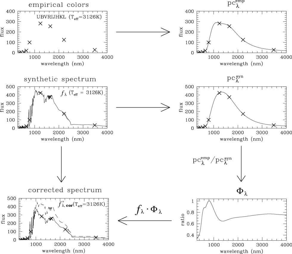
   Figure 10: Correction procedure. All fluxes are normalized to $f_{I}=100$.

   

   Figure 11: Correction functions for a range of effective temperatures.

5. Finally, the normalization of fluxes in the I–band, $f_{i}=100$, adopted initially for calculating the pseudo–continua must be cancelled now in order to restore the effective temperature scale. Thus, each corrected spectrum of the library, $f_{\lambda,corr}^{*}$ is scaled by a constant factor, $\xi(T,logg,\chi)$, to give the final corrected spectrum $f_{\lambda,corr}$:

   $$f_{\lambda,corr}(T,logg,\chi)=\xi(T,logg,\chi)\cdot f_{\lambda,corr}^{*}(T,logg,\chi),$$ (8)

   where

   $$\xi(T,logg,\chi)=\frac{\sigma T^{4}}{\int f_{\lambda}(T,logg,\chi)\cdot\Phi_{\lambda}(T)\cdot d\lambda}$$ (9)

   assures that the emergent integral flux of the final corrected spectrum conforms to the definition of the effective temperature (eqn. (1)).

Figure 12: Normalized corrected (solid lines) and original (dashed lines) library spectra for ranges in effective temperature and metallicity and covering wavelengths from the photometric U– through K–passbands. Top panels: K–library dwarf models; middle panels: K–library giant models; bottom panels: B+F–library giant models.

Figure 13: Same as Fig. 12, but for the visible–near infrared wavelength ranges only.

The final corrected spectra are thus in a format which allows immediate applications in population evolutionary synthesis. For a stellar model of given mass, metallicity, and age, the radius $R$ is determined by calculations of its evolutionary track in the theoretical HR diagram, and the total emergent flux at each wavelength can hence be obtained from the present library spectra via

$$F_{\lambda}(T,logg,\chi)=4\pi R^{2}\cdot f_{\lambda,corr}(T,logg,\chi).$$ (10)

5 Results: the corrected library spectra

We now discuss the properties of the new library spectra which result from the correction algorithm developed above, and which are most important in the context of population and evolutionary synthesis.

5.1 ${\rm T_{eff}}$–color relations

Fig. 14 illustrates the $T_{eff}$–color relations obtained after correction of the giant sequence spectra from the K– and B+F–libraries. Comparison with the corresponding Fig. 6 for the uncorrected spectra shows that the original differences which existed both between overlapping spectra of the two libraries and between the synthetic and empirical relations have indeed almost entirely been eliminated. While remaining differences between libraries are negligible, those between theoretical and empirical relations are below 0.1 mag.

Figure 14: Empirical color–effective temperature calibrations for solar–metallicity red giant stars (solid lines, according to Table 2) compared to the corresponding theoretical relations calculated from corrected synthetic library spectra (symbols, according to key in insert). Compare with Fig. 6.

Fig. 15 illustrates similar results for the main sequence. Again, comparison with the corresponding Fig. 7 before correction shows that the present calibration algorithm provides theoretical color–temperature relations which are in almost perfect agreement with the empirical data.

Figure 15: Empirical color–effective temperature calibrations for solar–metallicity dwarf stars (solid lines, see text for sources) compared to the corresponding theoretical relations calculated from corrected synthetic K–library spectra (symbols). Compare with Fig. 7.

Thus at this point, we can say that for solar abundances, the new library provides purely synthetic giant and dwarf star spectra that in general fit empirical color–temperature calibrations to within better than 0.1 mag over significant ranges of wavelengths and temperatures, and even to within a few hundredths of a magnitude for the hotter temperatures, $T_{eff}\geq 4000K$.

5.2 Bolometric corrections

Bolometric corrections, $BC_{V}$, are indispensable for the direct conversion of the theoretical HR diagram, $M_{bol}(T_{eff})$, into the observational color–absolute magnitude diagram, $M_{V}(B-V)$:

$$BC_{V}=M_{bol}-M_{V}+{\rm constant},$$ (11)

where the bolometric magnitude,

$$\begin{array}[]{rcl}M_{bol}&=&-2.5log\displaystyle\int_{0}^{\infty}f_{\lambda,corr}\,d\lambda\\ &&\\ &=&-2.5log(\sigma T_{eff}^{4}/\pi),\end{array}$$ (12)

provides the direct link to the effective temperature (scale). Of course, bolometric corrections applying to any other (arbitrary) passbands are then consistently calculated from $BC_{i}=BC_{V}+(M_{V}-M_{i})$, where the color $M_{V}-M_{i}$ is synthesized from the corrected library spectra.

Fig. 16 provides a representative plot of bolometric corrections, $BC_{V}$, for solar–abundance dwarf model spectra. The arbitrary constant in Eq. 11 has been defined in order to fix to zero the smallest bolometric correction (Buser & Kurucz 1978) found for the non-corrected models, which gives $BC_{\odot}=BC_{(5577,4.44,0.0)}=-0.190$. Comparison with the empirical calibration given by Schmidt-Kaler (1982) demonstrates that the present correction algorithm is reliable in this respect, too: predictions everywhere agree with the empirical data to within $\sim 0.05mag$ – which is excellent. Similar tests for the giant models also indicate that the correction procedure provides theoretical bolometric corrections in better agreement with the observations. These results will be discussed in a subsequent paper based on a more systematic application to multicolor data for cluster and field stars (Lejeune et al. 1997).

Figure 16: Bolometric correction, $BC_{V}$, as a function of effective temperature, for corrected K–library solar–metallicity dwarf model spectra. The solid line represents the empirical calibration given by Schmidt-Kaler (1982).

5.3 Grid of differential colors

Since comprehensive empirical calibration data have only been available for the full temperature sequences of solar–abundance giant and dwarf stars, direct calibration of the present library spectra using these data has, by necessity, also been limited to solar–abundance models. However, because one of the principal purposes of the present work has been to make available theoretical flux spectra covering a wide range in metallicities, it is important that the present calibration for solar–abundance models be propagated consistently into the remaining library spectra for parameter values ranging outside those represented by the calibration sequences. We thus have designed our correction algorithm in such a way as to preserve, at each temperature, the monochromatic flux ratios between the original spectra for different metallicities [M/H] and/or surface gravities log g. Justification of this procedure comes from the fact that, if used differentially, most modern grids of model–atmosphere spectra come close to reproducing observed stellar properties with relatively high systematic accuracy over wide ranges in physical parameters (e.g., Buser & Kurucz 1992, Lejeune & Buser 1996).

In order to check the extent to which preservation of monochromatic fluxes propagates into the broad–band colors, we have calculated the differential colors due to metallicity differences between models of the same effective temperature and surface gravity:

$$\Delta(c_{j,[M/H]})=c_{j,[M/H]}-c_{j,[M/H]=0},j=1,...,8.$$ (13)

We can then calculate the residual color differences between the corrected and the original grids:

$$\delta(\Delta(c_{j,[M/H]}))=\Delta(c_{j,[M/H]}^{corr})-\Delta(c_{j,[M/H]}^{orig}).$$ (14)

Results are presented in Figs. 17 and 18 for the coolest K–library models $(3500K\leq T_{eff}\leq 5000K)$ and for the B+F–library models for M giants $(2500K\leq T_{eff}\leq 3750K)$, respectively. Residuals are plotted as a function of the model number, which increases with both surface gravity and effective temperature, as given in the calibration sequences. The different lines represent different metallicities, $-3.0\leq[M/H]\leq+1.0$, as explained in the captions.

Figure 17: Residuals between differential colors obtained from original and corrected library spectra for models of the same effective temperatures and surface gravities but different metallicities. The abscissa represents the monotonic increase in temperature (as indicated along the top of the panel) and surface gravity in a similar way as Table 2. Residuals are for the coolest models from the K–library $(3500K\sim 5000K)$ and for metallicities $[M/H]=-3.0$ (solid line), $[M/H]=-1.0$ (long-dashed line), and $[M/H]=+1.0$ (dotted line).

Figure 18: Same as Fig. 17, but for the M–giant models from the B+K–library $(2500K\sim 3750K)$ and for metallicities $[M/H]=-1.0$ (solid line) and $[M/H]=+0.5$ (dotted line). The zero residuals for $U-B$ are due to the fact that in this wavelength range, B+K–library spectra are available for solar metallicity only.

The most important conclusion is that, in general, the correction algorithm does not alter the original differential grid properties significantly for most colors and most temperatures – in fact, the residuals are smaller than only a few hundredths of a magnitude. Typically, the largest residuals are found for the coolest temperatures $(T_{eff}\leq 3800K)$ and the shortest–wavelength colors, UBVRI, where the correction functions of Fig. 11 show the largest variations not only between the different passbands, but also within the individual passbands. This changes their effective wavelengths and, hence, the baselines defining the color scales (cf. Buser 1978). Since this effect tends to grow with the width of the passband, it is mainly the coincidence of large changes in both amplitudes and slopes of the correction functions with the wide–winged R–band which causes residuals for the R-I colors to be relatively large in Fig. 18.

Calculations of color effects induced by surface gravity changes lead to similar results. This corroborates our conclusion that the present correction algorithm indeed provides a new model spectra library which essentially incorporates, to within useful accuracy for the purpose, the currently best knowledge of fundamental stellar properties: a full–range color–calibration in terms of empirical effective temperatures at solar abundances (where comprehensive calibration data exist) and a systematic grid of differential colors predicted by the original theoretical model–atmosphere calculations for the full ranges of metallicities and surface gravities (where empirical data are still too scarce to allow comprehensive grid calibration).

Of course, we are aware that the present correction algorithm becomes increasingly inadequate with the complexity of the stellar spectra growing with decreasing temperature and/or increasing surface gravity and metallicity. For example, because under these conditions the highly nonlinear effects of blanketing due to line saturation and crowding and broad–band molecular absorption tend to dominate the behavior of stellar colors, particularly at shorter (i.e., visible) wavelengths, even the corresponding differential colors cannot either be recovered in a physically consistent manner by a simple linear model such as the present. However, the limits of this approach will be further explored in Paper II, where the calibration of theoretical spectra for M–dwarfs will be attempted by introducing the conservation of original differential colors of grid spectra as a constraint imposed to the correction algorithm.

6 Organization of the library

The corrected spectra have finally been composed into the unified library shown in Fig. 19. In this library, model spectra are given for a parameter grid which is uniformly sampled in $T_{eff}$, log g, and [M/H], each spectrum being available for the same wavelength grid, (${\rm 91\AA\leq\lambda\leq 1,600,000\AA}$), with a medium resolution of   10–20 Å.

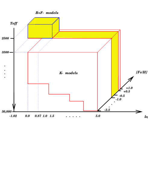
Figure 19: The $(\rm T_{eff},logg,[M/H])$ parameter space covered by the present unified library. Solid lines delineate approximate boundaries of available models. (B+F)–models for M–giants are confined to the metallicity range $-1.0\leq[M/H]\leq+0.5$ (grey part).

The main body consists of the K–library, which provides the most extensive coverage of parameter space (cf. Table 1) down to $T_{eff}=3500K$, and which has therefore been fully implemented to this limit. The extensions to lower temperatures, $3500K\geq T_{eff}\geq 2500K$, and associated lower surface gravities, $0.87\geq logg\geq-1.02$, are provided by the M–giant spectra from the B+F–library, which, however, covers only the limited metallicity range $+0.5\geq[M/H]\geq-1.0$.

This unified library is available (in electronic form) at the CDS, Strasbourg, France, where it can be obtained in either of two versions, with the corrected or the original uncorrected spectra from the K– and B+F–libraries.

7 Discussion and conclusion

Although astronomers have for a long time agreed that a uniform, complete, and realistic stellar library is urgently needed, it must be emphasized that this goal has remained too ambitious to be achieved in a single concerted effort through the present epoch. We have thus attempted to proceed in well–defined steps, with priorities set according to the availability of basic data and following the most obvious scientific questions that would likely become more tractable, or even answerable. Therefore, we briefly review the present achievement to clarify its status in the ongoing process toward a future standard library of theoretical stellar spectra for photometric evolutionary synthesis.

1. Completeness. The unification of the massive K–library spectra with those for high– luminosity M–star models (the B+F–library) is most important, because even as a small minority of the number population of a given stellar system, the late–type giants and supergiants may provide a large fraction of this system’s integrated light at visible and infrared wavelengths. This fact was recognized early on (e.g., Baum 1959), and eventually also co–motivated the effort leading to the existence of the B–library used in this work (Bessell et al. 1988).

   While the K–, B–, and F–libraries have been used to remedy incompleteness (in either wavelength or parameter coverage, or both) of available observed stellar libraries before (e.g., Worthey 1992, 1994; Fioc & Rocca–Volmerange 1996), our first goal here has been to join them as a purely theoretical library, providing the main advantages of physical homogeneity and definition in terms of fundamental stellar parameters – which allows direct use with stellar evolutionary calculations.

   But even so, the present library remains incomplete in several respects. First, stellar evolution calculations (e.g., Green et al. 1987) predict that high–luminosity stars with temperatures near or below $3500K$ may also exist at low metallicities, $[M/H]\sim-1.0$, and their flux contributions at visible–near ultraviolet wavelengths (where metallicity produces significant effects) may not quite be negligible in the integrated light of old stellar populations. Therefore, in order to provide the fuller coverage required for an adequate study of this metallicity–sensitive domain, new calculations of B–library spectra extending the original data to both shorter wavelengths $(\lambda\lambda\geq 320nm)$ and lower abundances $([M/H]\geq-2)$ (Buser et al. 1997) will replace the current hybrid B+F spectra and make the next library version more homogeneous.

   Secondly, even though the low–temperature, low–luminosity M–dwarf stars do not contribute significantly to the integrated bolometric flux, they are not negligible in the determination of mass–to–light ratios in stellar populations. Thus, a suitable grid of (theoretical) M–dwarf spectra calculated by Allard & Hauschildt (1995) is being subjected to a similar calibration process (Paper II) and will be implemented in the present library as an important step toward the intended standard stellar library.

   Finally, the libraries of synthetic spectra for hot O– and WR–stars which were recently calculated by Schmutz et al. (1992) will allow us to extend the calibration algorithm to ultraviolet IUE colors, where such stars radiate most of their light.
   

2. Realism. In view of its major intended application – photometric evolutionary synthesis –, the minimum requirement that we insist the theoretical library must satisfy, is to provide stellar flux spectra having (synthetic) colors which are systematically consistent with calibrations derived from observations. How else could we hope to learn the physics of distant stellar populations from their integrated colors, unless the basic building blocks – i.e., the library spectra used in the synthesis calculations – can be taken as adequate representations of the better–known fundamental stellar properties, such as their color–temperature relations?

   Because the original library spectra do not meet the above minimum requirement (Sect. 3), we have developed an algorithm for calibrating existing theoretical spectra against empirical color–temperature relations (Sect. 4). Because comprehensive empirical data are unavailable for large segments of the parameter space covered by the theoretical library, direct calibration can be effected only for the major sequences of solar–abundance models (Sect. 5). However, we have also shown that the present algorithm provides the desired broad–band (or pseudo–continuum) color calibration without destroying the original relative monochromatic fluxes between arbitrary model grid spectra and solar–abundance calibration sequence spectra of the same effective temperature. This conservation of original grid properties also propagates with useful systematic accuracy even through most differential broad–band colors of the corrected library spectra. Thus, to the extent that differential broad–band colors of original library spectra were previously shown to be consistent with spectroscopic or other empirical calibrations of the UBV–, RGU–, and Washington ultraviolet-excess–metallicity relations (Buser & Fenkart 1990, Buser & Kurucz 1992, Lejeune & Buser 1996), the corrected library spectra are still consistent with the same calibrations.
   

3. Library development. At this point, we feel that some of the more important intrinsic properties required of the future standard library have already been established. Of course, many more consistency tests and calibrations will now be needed that can, however, only be performed for local volumes of the full parameter space covered by the new library. For example, we shall use libraries of observed flux spectra for individual field and cluster stars to better assess – and/or improve – the performance of the present library version in the non–solar–abundance and non–visual wavelength regimes. Eventually, we also expect significant guidance toward a more systematically realistic version of the library from actual evolutionary synthesis calculations of the integrated spectra and colors of globular clusters (Lejeune 1997).

   Last, but not least, we would like to emphasize that, while we here present the results taylored according to the general needs in the field of photometric evolutionary synthesis, the library construction algorithm has been designed such as to allow flexible adaptation to alternative calibration data as well. As we shall ourselves peruse this flexibility to accommodate both feed–back and new data, the reader, too, is invited to define his or her own preferred calibration constraints and have the algorithm adapted to perform accordingly.

Acknowledgements. We are grateful to Michael Scholz and Gustavo Bruzual for providing vital input and critical discussions. Christophe Pichon is also aknowledged for his precious help with the final implementation of some of the figures. We wish to thank warmly the referee for his helpful comments and suggestions. This work was supported by the Swiss National Science Foundation.

References

- [1] Allard F., Hauschildt P.H., 1995, ApJ, 445, 433
- [2] Baum W. A., 1959, PASP, 71, 106
- [3] Bell R.A., Eriksson K., Gustafsson B., Nordlund A., 1976, A&AS 23, 37
- [4] Bessell M.S., 1979, PASP, 91, 589
- [5] Bessell M.S., Brett J.M., 1988, PASP, 100, 1134
- [6] Bessell M.S., Brett J.M., Scholz M., Wood P.R., 1989, A&AS, 77, 1
- [7] Bessell M.S., Brett J.M., Scholz M., Wood P.R., 1991, A&AS, 89, 335
- [8] Bruzual G.A., 1995, private communication
- [9] Bruzual G.A., Charlot S., 1993, ApJ, 405, 538
- [10] Bruzual G.A. et al., 1997 (in preparation)
- [11] Buser R., 1978, A&A, 62, 411
- [12] Buser R., Fenkart, R.P. 1990, A&A 239, 243
- [13] Buser R., Kurucz R., 1978, A&A, 70, 555
- [14] Buser R., Kurucz R., 1992, A&A, 264, 557
- [15] Buser R., Scholz M., Lejeune Th. 1997, A&A (in preparation)
- [16] Eriksson K., Bell R.A., Gustafsson B., Nordlund A., 1979, Trans. IAU Vol. 17A, Part 2, Reidel, Dordrecht, p. 200
- [17] Fioc M., Rocca–Volmerange B., 1996, A&A, submitted
- [18] FitzGerald M.P., 1970, A&A, 4, 234
- [19] Fluks M.A. et al., 1994, A&AS, 105, 311
- [20] Green E.M., Demarque P., King C.R., 1987, The Revised Yale Isochrones and Luminosity Functions, Yale Univ. Obs., New Haven, USA
- [21] Gustafsson B., Bell R.A., Eriksson K., Nordlund A., 1975, A&A 42, 407
- [22] Johnson H.L., 1966, ARA&A 4, 193
- [23] Kurucz R.L., 1979a, ApJS, 40, 1
- [24] Kurucz R.L., 1979b, in: Problems of Calibration of Multicolor Photometric Systems, ed. A.G. Davis Philip, Dudley Obs. Rep. 14, p. 363
- [25] Kurucz R.L., 1992, in: The Stellar Populations of Galaxies, eds. B. Barbuy, A. Renzini, IAU Symp. 149, Dordrecht, Kluwer, p. 225
- [26] Kurucz R., 1995, CD–ROM, private communication
- [27] Kurucz R.L., Peytremann E., 1975, Smithsonian Astrophys. Obs. Special Rep. 362
- [28] Leitherer C. et al., 1996, PASP 108, 996
- [29] Lejeune Th., 1997, Ph.D. thesis, in preparation
- [30] Lejeune Th., Buser R., 1996, Baltic Astronomy, 5, 399
- [31] Lejeune Th., Buser R., Cuisinier F. 1997, A&A (in preparation, Paper II)
- [32] Lejeune Th., Lastennet E., Valls-Gabaud D, Buser R. 1997, A&A (in preparation)
- [33] Plez, B., Brett, J., Nordlund, A., 1992, A&A 256, 551
- [34] Ridgway S.T., Joyce R.R., White N.M., Wing R.F., 1980, ApJ, 235, 126
- [35] Schaller G., Schaerer D., Meynet G., Maeder A., 1992, A&AS, 96, 269
- [36] Schmidt-Kaler, Th., 1982, in:Landolt-Börstein, Neue Serie, Gruppe VI, Bd. 2b, eds. K Schaifers, H.H. Voigt, Springer, Berlin Heidelberg New York, p. 14
- [37] Schmutz W., Leitherer C., Gruenwald R., 1992, PASP, 104, 682
- [38] Worthey G., 1992, PhD thesis, Univ. of California, Santa Cruz
- [39] Worthey G., 1994, ApJS, 95, 107