Maximum-Likelihood Comparisons of Tully-Fisher
and Redshift Data: Constraints on $\Omega$ and Biasing

Abstract

We compare Tully-Fisher (TF) data for 838 galaxies within $cz=3000\ {\rm km}\,{\rm s}^{-1}$ from the Mark III catalog to the peculiar velocity and density fields predicted from the 1.2 Jy IRAS redshift survey. Our goal is to test the relation between the galaxy density and velocity fields predicted by gravitational instability theory and linear biasing, and thereby to estimate $\beta_{I}\equiv\Omega^{0.6}/b_{I},$ where $b_{I}$ is the linear bias parameter for IRAS galaxies on a 300 km s^-1 scale. Adopting the IRAS velocity and density fields as a prior model, we maximize the likelihood of the raw TF observables, taking into account the full range of selection effects and properly treating triple-valued zones in the redshift-distance relation. Extensive tests with realistic simulated galaxy catalogs demonstrate that the method produces unbiased estimates of $\beta_{I}$ and its error. When we apply the method to the real data, we model the presence of a small but significant velocity quadrupole residual ($\sim\,$3.3% of Hubble flow), which we argue is due to density fluctuations incompletely sampled by IRAS. The method then yields a maximum likelihood estimate $\beta_{I}=0.49\pm 0.07$ ($1\,\sigma$ error). We discuss the constraints on $\Omega$ and biasing that follow from this estimate of $\beta_{I}$ if we assume a COBE-normalized CDM power spectrum. Our model also yields the one dimensional noise in the velocity field, including IRAS prediction errors, which we find to be $125\pm 20\ {\rm km}\,{\rm s}^{-1}.$

We define a $\chi^{2}$-like statistic, $\chi^{2}_{\xi},$ that measures the coherence of residuals between the TF data and the IRAS model. In contrast with maximum likelihood, this statistic can identify poor fits, but is relatively insensitive to the best $\beta_{I}.$ As measured by $\chi^{2}_{\xi},$ the IRAS model does not fit the data well without accounting for the residual quadrupole; when the quadrupole is added the fit is acceptable for $0.3\leq\beta_{I}\leq 0.9$. We discuss this in view of the Davis, Nusser, & Willick analysis that questions the consistency of the TF and IRAS data.

1 Introduction

One of the most important tasks facing observational cosmology is determination of the density parameter $\Omega.$ Along with the Hubble constant $H_{0}$ and the cosmological constant $\Lambda,$ the density parameter fixes the global structure of spacetime. One approach to the problem uses the classical cosmological tests of the geometry of the universe, such as the apparent magnitudes as a function of redshift of standard candles (e.g., Type Ia Supernovae, Perlmutter et al. 1996). While promising, this approach is sensitive to the possible evolution of the standard candles with redshift. Moreover, it is difficult to disentangle the effects of $\Lambda$ and $\Omega$ in such tests (Dekel, Burstein, & White 1997). Alternatively, one may carry out dynamical measurements of $\Omega$ in the local ($z\lower 2.15277pt\hbox{$\,\buildrel<\over{\sim}\,$}0.05$) universe, in which both evolution and the geometrical effects of the cosmological constant may be safely neglected.

Low-redshift tests of $\Omega$ are based on dynamical measurements of the mass of gravitating matter on some characteristic size scale. For example, measurements of rotation curves (Rubin 1983) or the motions of satellite galaxies (Zaritsky et al. 1993) yield the masses of ordinary spirals within $\sim\,$10–200 kpc of their centers. The velocity dispersions (Carlberg et al. 1996), X-ray temperatures (White et al. 1993), and gravitational lensing effects (Tyson & Fischer 1995; Squires et al. 1996) of rich clusters of galaxies provide mass estimates on $\sim\,$1 Mpc scales. In general, these and other dynamical analyses of matter in the highly clustered regime have pointed to a mass density corresponding to $\Omega\simeq 0.2\pm 0.1$ (e.g., Bahcall, Lubin, & Dorman 1995). This value exceeds that implied by known sources of luminosity ($\Omega_{{\rm lum}}\lower 2.15277pt\hbox{$\,\buildrel<\over{\sim}\,$}0.01;$ Peebles 1993) or inferred from primordial nucleosynthesis ($\Omega_{{\rm baryon}}\lower 2.15277pt\hbox{$\,\buildrel<\over{\sim}\,$}0.05;$ Turner et al. 1996), and thus points to the existence of nonbaryonic dark matter. However, it is well below the Einstein-de Sitter value of $\Omega=1$ that is favored by simplicity and coincidence arguments (e.g., Dicke 1970). The natural expectation from the inflation scenario is that the universe is flat, $\Omega+\Omega_{\Lambda}=1$, where $\Omega_{\Lambda}\equiv\Lambda/3H_{0}^{2}$ is the effective energy density contributed by a cosmological constant (Guth 1981; Linde 1982; Albrecht & Steinhardt 1982). However, if $\Omega\simeq 0.2,$ this inflationary prediction requires $\Omega_{\Lambda}\simeq 0.8,$ which conflicts with upper limits obtained from studies of gravitational lensing (Carroll, Press, & Turner 1992; Maoz & Rix 1993; Kochanek 1996).

It is possible, however, that $\Omega$ could be close to or exactly equal to unity despite evidence to the contrary from dynamical tests on $\sim\,$1 Mpc scales. This could occur if the dark matter is poorly traced by dense concentrations of luminous matter such as galaxies and galaxy clusters. If so, dynamical tests on scales $\lower 2.15277pt\hbox{$\,\buildrel>\over{\sim}\,$}10$ Mpc are necessary to obtain an unbiased estimate of $\Omega.$ Such tests involve measurements of the coherent, large-scale peculiar velocities of galaxies. According to gravitational instability theory (cf. Eq. 1), these motions are related in an $\Omega$-dependent way to the large-scale distribution of mass. If the latter, in turn, can be inferred from the observed distribution of galaxies on large scales, one might hope to derive an estimate of $\Omega$ that is free from the pitfalls of small-scale dynamical analyses.

This program requires a comparative analysis of two types of data sets. The first consists of radial velocities and redshift-independent distance estimates for large samples of galaxies. The largest such compilation to date is the Mark III catalog (Willick et al. 1997), which contains distance estimates for $\sim\,$3000 spiral galaxies from the Tully-Fisher (1977; TF) relation, and for 544 elliptical galaxies from the $D_{n}$-$\sigma$ relation (Djorgovski & Davis 1987; Dressler et al. 1987). The second type of data set is a full-sky redshift survey with well-understood selection criteria. Several large redshift surveys exist (cf. Strauss & Willick 1995, hereafter SW, and Strauss 1996a, for reviews); the one which most nearly meets the requirements of full-sky coverage and well-understood selection is the IRAS 1.2 Jy survey (Fisher et al. 1995). The basic idea behind the comparison is as follows. In the linear regime (mass density fluctuations $\delta\equiv\delta\rho/\rho_{0}\ll 1$), the global relationship between the peculiar velocity field ${\bf v}({\bf r})$ and the mass-density fluctuation field $\delta({\bf r})$ is given by gravitational instability theory:

$${\bf v}({\bf r})=\frac{f(\Omega)}{4\,\pi}\int d^{3}{\bf r}^{\prime}\,\frac{\delta({\bf r}^{\prime})({\bf r}^{\prime}-{\bf r})}{\left|{\bf r}^{\prime}-{\bf r}\right|^{3}}\,,$$ (1)

where $f(\Omega)\approx\Omega^{0.6}$ (Peebles 1980). If mass density fluctuations are equal to galaxy number density fluctuations, at least on the scales ($\,\buildrel>\over{\sim}\,$ few Mpc) over which it is possible to define continuous density fields, then the redshift survey data yield a map of $\delta({\bf r})$ (after correction for peculiar velocities; Appendix A). By Eq. (1), one then derives a predicted peculiar velocity field ${\bf v}({\bf r})$ as a function of $\Omega.$ The TF or $D_{n}$-$\sigma$ data provide the observed peculiar velocities. The best estimate of $\Omega$ is the one for which the predicted and observed peculiar velocities best agree.

Two obstacles make this comparison a difficult one. The first, already alluded to, is fundamental: one observes galaxy number density ($\delta_{g}$) rather than mass density ($\delta$) fluctuations. A model is required for relating the first to the second. The simplest approximation is linear biasing,

$$\delta_{g}({\bf r})=b\,\delta({\bf r}),$$ (2)

in which the bias parameter $b$ is assumed to be spatially constant. Substituting Eq. (2) in Eq. (1) yields

$${\bf v}({\bf r})=\frac{\beta}{4\,\pi}\int d^{3}{\bf r}^{\prime}\,\frac{\delta_{g}({\bf r}^{\prime})({\bf r}^{\prime}-{\bf r})}{\left|{\bf r}^{\prime}-{\bf r}\right|^{3}}\,,$$ (3)

where $\beta\equiv f(\Omega)/b.$ Thus, under the dual assumptions of linear dynamics and linear biasing, comparisons of peculiar velocity and redshift survey data, by themselves, can yield the parameter $\beta$ but not $\Omega.$ One might hope to break the $\Omega$-$b$ degeneracy by generalizing Eq. (1) to the nonlinear dynamical regime (cf. Dekel 1994, § 2, or Sahni & Coles 1996, for a review). However, such generalizations are difficult to implement in practice; furthermore, nonlinear extensions to Eq. (2) will enter to the same order as nonlinear dynamics (we discuss this issue further in § 6.3.1). Thus, without a more realistic a priori model of the relative distribution of galaxies versus mass, it is prudent to limit the goals of the peculiar velocity-redshift survey comparison to testing gravitational instability theory and determining $\beta.$ One may then adduce external information on the value of $b$ to place constraints on $\Omega$ itself.

The second obstacle is the sheer technical difficulty of the problem. The redshift-independent distances obtained from methods such as TF are large ($\sim\,$20%; Willick et al. 1996), and are subject to potential systematic errors due to statistical bias effects (Dekel 1994; SW, § 6). Furthermore, we measure the galaxy density field $\delta_{g}$ in redshift space, whereas it is the real-space density that yields peculiar velocities via Eq. (3). The relationship between the two depends on the peculiar velocity field itself. Self-consistent methods, in which ${\bf v}_{p}$ is both the desired end product and a necessary intermediate ingredient in the calculation, must therefore be developed for predicting peculiar velocities from redshift surveys (Appendix A). For these reasons, reliable comparisons of peculiar velocity and redshift survey data require extremely careful statistical analyses.

This problem has inspired a number of independent approaches in recent years. The POTENT method (Dekel, Bertschinger, & Faber 1990; Dekel 1994; Dekel et al. 1997) was the first effort at a rigorous treatment of peculiar velocity data. Dekel et al. (1993) compared the POTENT reconstruction of the Mark II peculiar velocity data (Burstein 1989) to the IRAS 1.936 Jy redshift survey (Strauss et al. 1992b), finding $\beta_{I}=1.28^{+0.75}_{-0.59}$ at 95% confidence. An improved treatment using the Mark III peculiar velocities (Willick et al. 1997) and the IRAS 1.2 Jy survey (Fisher et al. 1995) yields $\beta_{I}=0.86\pm 0.15$ (Sigad et al. 1997, hereafter POTIRAS). Hudson et al. (1995) compared the optical redshift survey data of Hudson (1993) to the POTENT reconstruction based on a preliminary version of the Mark III catalog, finding $\beta_{{\rm opt}}=0.74\pm 0.13$ ($1\,\sigma$ errors). These results from POTENT were obtained using 1200 km s^-1 Gaussian smoothing. A distinct approach, which differs from POTIRAS in the statistical biases to which it is vulnerable (SW), and which typically uses much smaller smoothing, is to predict galaxy peculiar velocities and thus distances from the density field, and then use these predictions to minimize the scatter in the TF or $D_{n}$-$\sigma$ relations (Strauss 1989; Hudson 1994; Roth 1994; Schlegel 1995; Shaya, Peebles, & Tully 1995; Davis, Nusser, & Willick 1996, hereafter DNW). This second kind of analysis has produced estimates of $\beta_{I}$ in the range $\sim\,$0.4–0.7, lower than the values obtained from POTIRAS. We further clarify the distinction between the two methods in § 2.1, and discuss possible reasons for the discrepancies in § 6.1.

In this paper, we present a new maximum-likelihood method for comparing TF data to the predicted peculiar velocity and density fields in order to estimate $\beta.$ Its chief strength is an improved treatment of nearby galaxies $(cz\leq 3000\ {\rm km}\,{\rm s}^{-1})$, and we limit the analysis to this range. The TF data we use comprise a subset of the Mark III catalog of Willick et al. (1997). The predicted peculiar velocities are obtained using new reconstruction methods (Appendix A) from the IRAS 1.2 Jy redshift survey. The outline of this paper is as follows. In § 2, we first review the strengths and weaknesses of existing approaches, and then describe our new method in detail. In § 3, we present tests of the method using mock catalogs. In § 4, we apply the method to the Mark III catalog and obtain an estimate of $\beta_{I}.$ In § 5, we analyze residuals from our maximum likelihood solution in order to assess whether IRAS predictions give a statistically acceptable fit to the Mark III data. In § 6, we further discuss and summarize our principal results. This paper is the product of nearly three years work and contains considerable detail. We recommend that readers interested primarily in results and interpretation skim § 2, and then read § 3.1, 4.4, 4.5, 5.1, 5.2, and 6.4.

2 Description of the Maximum Likelihood Method

2.1 Alternative Approaches to the Peculiar Velocity-Density Comparison

Before presenting our method in detail, we briefly review the principal alternatives. Two approaches are fairly paradigmatic, and serve to illustrate the main issues and motivate our approach. These are the POTENT method of Dekel and coworkers (e.g., Dekel 1994; Dekel et al. 1997) mentioned in § 1, and the ITF method of Nusser & Davis (Nusser & Davis 1995; DNW).

The POTENT algorithm is designed to reconstruct, from sparse and noisy radial peculiar velocity estimates, a smooth three-dimensional peculiar velocity field and the associated mass density field. The method is based on the property that the smoothed velocity field of gravitating systems is the gradient of a potential. The divergence of Eq. (3) is

$$\nabla\cdot{\bf v}=-\beta\delta_{g}\,.$$ (4)

Thus, $\beta$ is the slope of the correlation between $\nabla\cdot{\bf v},$ obtained from POTENT, and $\delta_{g}$ obtained from redshift survey data. This is the basis of the POTIRAS approach to determining $\beta_{I},$ discussed above (§ 1).

POTENT has several advantages as a reconstruction method. It yields model-independent, three-dimensional velocity and density fields well-suited for comparison with theory and for visualization. It works in the space of TF-inferred distances, i.e., it is a Method I approach to velocity analysis (cf. SW, § 6.4.1). Unlike Method II approaches (see below), it does not assume that there is a unique distance corresponding to a given redshift. In regions where galaxies at different distances are superposed in redshift space, POTENT is capable of recovering the true velocity field. The POTIRAS comparison between the mass and galaxy density fields is entirely local (Eq. 4), whereas predicted peculiar velocities are highly nonlocal (Eq. 3). Locality ensures that biases due to unsampled regions are minimized.

The liabilities of POTENT are closely related to its strengths. In order to construct a model-independent velocity field it must have redshift-independent distances as input. Such distances require properly calibrated TF relations. In particular, the TF distances for samples that probe different regions of the sky must be brought to a uniform system, which is a difficult procedure (cf. Willick et al. 1995, 1996, 1997). Errors made in calibrating and homogenizing the TF relations will propagate into the POTENT velocity field. Because POTENT works in inferred distance space, it is subject to inhomogeneous Malmquist bias (Dekel, Bertschinger, & Faber 1990). Minimizing this bias requires significant smoothing of the input data. POTENT currently employs a Gaussian smoothing scale of 1000–1200 km s^-1 (Dekel 1994; Dekel et al. 1997), making it relatively insensitive to dynamical effects on small scales. As a result, the current POTENT applications are not particularly effective at extracting detailed information from the velocity field in the local ($cz\lower 2.15277pt\hbox{$\,\buildrel<\over{\sim}\,$}3000\ {\rm km}\,{\rm s}^{-1}$) universe.

DNW take a different approach. They work with the “inverse” form of the TF relation (Dekel 1994, § 4.4; SW, § 6.4.4), and thus refer to their method as ITF. They express peculiar velocity as a function of redshift-space, rather than real-space, position; in the terminology of SW, ITF is thus a Method II analysis, largely impervious to inhomogeneous Malmquist bias. DNW expand the redshift-space peculiar velocity field in a set of independent basis functions, or modes, whose coefficients are solved for simultaneously with the parameters of a global inverse TF relation via $\chi^{2}$ minimization of TF residuals. The TF data are never converted into inferred distances and thus do not require pre-calibrated TF relations. The IRAS-predicted velocity field is expanded in the same set of basis functions, allowing a mode-by-mode comparison of predicted and observed peculiar velocities. This ensures that one is comparing quantities that have undergone the same spatial smoothing, a desirable characteristic of the fit.

As with POTENT, the strengths of ITF are connected with certain disadvantages. Because it is a Method II approach, multivalued or flat zones in the redshift-distance relation (see below) necessarily bias the ITF analysis. It neglects the role of small-scale velocity noise, which is non-negligible for galaxies within 1000 km s^-1. These features make ITF, like POTENT, a relatively ineffective tool for probing the very local region. Last and most importantly, the ITF method as implemented by DNW requires that the raw magnitude and velocity width data from several distinct data sets be carefully matched before being input to the algorithm. Any systematic errors incurred in matching the raw data from different parts of the sky will induce large-scale, systematic errors in the derived velocity field. Thus, although ITF does not need input TF distances, it is vulnerable to a priori calibration errors just as POTENT is.

2.2 VELMOD

The approach we take in this paper, “VELMOD,” is a maximum likelihood method designed to surmount several of the difficulties that face POTIRAS and ITF. VELMOD generalizes and improves upon the Method II approach to velocity analysis. Method II takes as its basic input the TF observables (apparent magnitude and velocity width) and redshift of a galaxy, and asks, what is the probability of observing the former, given the value of the latter? It then maximizes this probability over the entire data set with respect to parameters describing the TF relation and the velocity field. The underlying assumption of Method II is that a galaxy’s redshift, in combination with the correct model of the velocity field, yields its true distance, which then allows the probability of the TF observables to be computed. This analytic approach was originally developed by Schechter (1980), and was later used by Aaronson et al. (1982b), Faber & Burstein (1988), Strauss (1989), Han & Mould (1990), Hudson (1994), Roth (1994), and Schlegel (1995), among others.

The main problem with Method II is its assumption that a unique redshift-distance mapping is possible. This assumption breaks down for two reasons. First, redshift is a “noisy” realization of distance plus predicted peculiar velocity—both because of true velocity noise generated on very small ($\lower 2.15277pt\hbox{$\,\buildrel<\over{\sim}\,$}\,1$ Mpc) scales, and because of the inaccuracy of the velocity model (even for the correct $\beta$) due to nonlinear effects and shot noise in the density field. Second, even in the absence of noise, the redshift-distance relation can, in principle, be multivalued: more than one distance along the line of sight can correspond to a given redshift. VELMOD accounts for all of these effects statistically by replacing the unique distance of Method II with the joint probability distribution of redshift and distance. This distribution is constructed to allow for both noise and multivaluedness. The distance dependence is then integrated out (§ 2.2.1), yielding the correct probability distribution of the TF observables given redshift.

There are two additional advantages to the VELMOD approach. First, it requires neither a priori calibration of the TF relations (as does POTENT) nor matching of the input data from disparate samples (as does ITF). An individual TF calibration for each independent sample occurs naturally as part of the analysis. Second, it does not require smoothing of the input TF data, and thus allows as high-resolution an analysis as the data intrinsically permit. This second feature, along with its allowance for velocity noise and triple-valued zones, makes VELMOD well-suited for probing the local ($cz\lower 2.15277pt\hbox{$\,\buildrel<\over{\sim}\,$}3000\ {\rm km}\,{\rm s}^{-1}$) velocity field. An analysis of local data is desirable because random and systematic errors in both the IRAS and TF data are less important nearby than far away.

2.2.1 Mathematical Details

We now describe the method in detail. We assume that the relevant distance indicator is the TF relation; with minor changes the formalism could be adapted to comparable distance indicators such as $D_{n}$-$\sigma$. We use the terminology of Willick (1994) and Willick et al. (1995): briefly, we denote by $m$ and $\eta\equiv\log v_{\rm rot}-2.5$ a galaxy’s corrected apparent magnitude and velocity width parameter, respectively; by $cz$ its Local Group frame radial velocity (“redshift”) in km s^-1; and by $r$ its true distance in km s^-1. We define the distance modulus as $\mu\equiv 5\log r,$ and absolute magnitudes as $M=m-\mu.$ We write the forward and inverse TF relations as linear expressions, $M(\eta)=A-b\eta$ and $\eta^{0}(M)=-e(M-D),$ and denote their rms scatters $\sigma_{{\rm TF}}$ and $\sigma_{\eta},$ respectively.

We seek an exact expression for the probability that a galaxy at redshift $cz$ possesses TF observables $(m,\eta)$ given a model of the peculiar velocity and density fields. We first consider the joint probability distribution of the TF observables, redshift, and an unobservable quantity, the true distance $r.$ Later, we will integrate over $r$ to obtain the probability distribution of the observables. We may write

$$P(m,\eta,cz,r)=P(m,\eta|r)\times P(cz|r)\times P(r)\,.$$ (5)

The splitting into conditional probabilities reflects the fact that the TF observables and the redshift couple with one another only via their individual dependences on the true distance $r.$

The first of the three terms on the right hand side of Eq. (5) depends on the luminosity function, the sample selection function, and the TF relation. We can express it in one of two ways, depending on whether we are using the forward or inverse form of the TF relation:

1. Forward relation:

   $$P(m,\eta|r)\propto\phi(\eta)S(m,\eta,r){1\over\sigma_{{\rm TF}}}\exp\!\left(-\frac{\left[m-(M(\eta)+\mu(r))\right]^{2}}{2\sigma_{{\rm TF}}^{2}}\right)$$ (6)

2. Inverse relation:

   $$P(m,\eta|r)\propto\Phi(m-\mu(r))S(m,\eta,r){1\over\sigma_{\eta}}\exp\!\left(-\frac{\left[\eta-\eta^{0}(m-\mu(r))\right]^{2}}{2\sigma_{\eta}^{2}}\right)\,,$$ (7)

where $\phi(\eta)$ and $\Phi(M)$ are the (closely related) velocity width distribution function and luminosity function, $S(m,\eta,r)$ is the sample selection function, and we have assumed Gaussian scatter of the TF relation (an assumption validated by Willick et al. 1997). Detailed derivations of these expressions are given by Willick (1994). In Eqs. (6) and (7) we have written only proportionalities, as the normalization is straightforward and will occur at a later point in any case.

The third term on the right hand side of Eq. (5) is simply the a priori probability of observing an object at distance $r,$

$$P(r)\propto r^{2}n(r)\,,$$ (8)

where $n(r)\propto 1+\delta_{g}({\bf r})$ is the number density of the species of galaxies that makes up the sample. The second term on the right hand side of Eq. (5), $P(cz|r),$ is the one which couples the TF observables to the velocity field model. We assume that, for the correct IRAS velocity field reconstruction (i.e., for the correct value of $\beta_{I}$ and other velocity field parameters to be described below), the redshift is normally distributed about the value predicted from the velocity model:

$$P(cz|r)=\frac{1}{\sqrt{2\pi}\,\sigma_{v}}\exp\!\left(-\frac{[cz-(r+u(r))]^{2}}{2\sigma_{v}^{2}}\right)\,,$$ (9)

where $u(r)\equiv\hat{\bf r}\cdot\left[{\bf v}({\bf r})-{\bf v}({\bf 0})\right]$ is the radial component of the predicted peculiar velocity field in the Local Group frame (cf. Eq. 30). We treat the velocity noise $\sigma_{v}$ as a free parameter in our analysis; we discuss its origin in detail in § 3.2. Although $\sigma_{v}$ must be position or density dependent at some level, we treat it as spatially constant in this paper, except in the Virgo cluster (§ 4.3).

Substituting Eqs. (6) or (7), (8), and (9) into Eq. (5) yields the joint probability distribution $P(m,\eta,cz,r).$ To obtain the joint probability distribution of the observable quantities, one integrates over the (unobserved) line-of-sight distance, i.e.,

$$P(m,\eta,cz)=\int_{0}^{\infty}P(m,\eta,cz,r)\,dr\,.$$ (10)

In practice, it is not optimal to base a likelihood analysis on the joint distribution $P(m,\eta,cz)$ because of its sensitivity to terms, such as the luminosity function, the sample selection function, and the density field, that are not critical for our purposes. Instead, the desired probability distributions are the conditional ones:

1. Forward TF relation:

   $$P(m|\eta,cz)\,=\,\frac{P(m,\eta,cz)}{\int_{-\infty}^{\infty}P(m,\eta,cz)\,dm}$$

   $$=\frac{\int_{0}^{\infty}\!dr\,r^{2}n(r)\,P(cz|r)\,S(m,\eta,r)\exp\!\left(-\frac{\left[m-(M(\eta)+\mu(r))\right]^{2}}{2\sigma_{{\rm TF}}^{2}}\right)}{\int_{0}^{\infty}\!dr\,r^{2}n(r)\,P(cz|r)\,\int_{-\infty}^{\infty}\!dm\,S(m,\eta,r)\exp\!\left(-\frac{\left[m-(M(\eta)+\mu(r))\right]^{2}}{2\sigma_{{\rm TF}}^{2}}\right)}\,;$$ (11)

2. Inverse TF relation:

   $$P(\eta|m,cz)\,=\,\frac{P(m,\eta,cz)}{\int_{-\infty}^{\infty}P(m,\eta,cz)\,d\eta}$$

   $$=\frac{\int_{0}^{\infty}\!dr\,r^{2}n(r)\,\Phi(m-\mu(r))\,P(cz|r)\,S(m,\eta,r)\exp\!\left(-\frac{\left[\eta-\eta^{0}(m-\mu(r))\right]^{2}}{2\sigma_{\eta}^{2}}\right)}{\int_{0}^{\infty}\!dr\,r^{2}n(r)\,\Phi(m-\mu(r))\,P(cz|r)\,\int_{-\infty}^{\infty}\!d\eta\,S(m,\eta,r)\exp\!\left(-\frac{\left[\eta-\eta^{0}(m-\mu(r))\right]^{2}}{2\sigma_{\eta}^{2}}\right)}\,,$$ (12)

where $P(cz|r)$ is given by Eq. (9). Although neither of these expressions is independent of the density field $n(r)$ or the selection function $S$, their appearance in both the numerator and denominator much reduces their sensitivity to them. A similar statement holds for the luminosity function $\Phi$ in Eq. (12). The velocity width distribution function $\phi$ has, however, dropped out entirely from the forward relation probability. We discuss these points further in § 2.2.2.

Equations (11) and (12) are the conditional probabilities whose products over all galaxies in the sample we wish to maximize. In practice, we do so by minimizing the quantities

$${\cal L}_{{\rm forw}}=-2\sum_{i}\ln P(m_{i}|\eta_{i},cz_{i})$$ (13)

or

$${\cal L}_{{\rm inv}}=-2\sum_{i}\ln P(\eta_{i}|m_{i},cz_{i})\,,$$ (14)

where the index $i$ runs over all objects in the TF sample. We have assumed that the probabilities for each galaxy are independent; we validate this assumption a posteriori (cf. § 5.2).

2.2.2 Further discussion of the VELMOD likelihood

The physical meaning of the VELMOD likelihood expressions is clarified by considering them in a suitable limit. If we take $\sigma_{v}$ to be “small,” in a sense to be made precise below, the integrals in Eqs. (11) and (12) may be approximated using standard techniques. If in addition we neglect sample selection ($S=1$) and density variations ($n(r)=\rm constant$), and assume that the redshift-distance relation is single-valued, we find for the forward relation:

$$P(m|\eta,cz)\simeq\frac{1}{\sqrt{2\pi}\sigma_{e}}\,\exp\left\{-\frac{1}{2\sigma_{e}^{2}}\left(m-\left[M(\eta)+5\log w+\frac{10}{\ln 10}\Delta_{v}^{2}\right]\right)^{2}\right\}\,,$$ (15)

where $w$ is the solution to the equation $cz=w+u(w),$ i.e., it is the distance inferred from the redshift and peculiar velocity model; $\Delta_{v}\equiv\sigma_{v}/[w(1+u^{\prime})],$ where $u^{\prime}=\left(\partial u/\partial r\right)_{r=w},$ is the effective logarithmic velocity dispersion; and

$$\sigma_{e}\equiv\left[\sigma_{{\rm TF}}^{2}+\left(\frac{5}{\ln 10}\right)^{2}\Delta_{v}^{2}\right]^{1/2}$$ (16)

is the effective TF scatter, including the contribution due to $\sigma_{v}.$ An analogous result holds for the inverse relation. The criterion $\Delta_{v}^{2}\ll 1,$ which quantifies the statement that $\sigma_{v}$ is “small,” must be satisfied to derive Eq. (15).

Eq. (15) shows that the probability distribution $P(m|\eta,cz)$ preserves the Gaussian character of the real-space TF probability distribution $P(m|\eta,r)$ in this limit. However, the expected value of $m$ is shifted from the “naïve” value $M(\eta)+5\log w$ by an amount $\sim 4.3\Delta_{v}^{2}.$ This shift is in fact nothing more than the homogeneous Malmquist bias due to small-scale velocity noise; it differs in detail from the usual Malmquist expression (i.e., that which affects a Method I analysis) because it arises from the Gaussian (rather than log-normal) probability distribution, Eq. (9). Furthermore, the effective scatter $\sigma_{e}$ is larger than $\sigma_{{\rm TF}}$, because the velocity dispersion introduces additional distance error and thus magnitude scatter. The effects associated with velocity noise diminish with distance ($\Delta_{v}\propto r^{-1}$), however; the velocity Malmquist effect vanishes in the limit of large distances, in contrast with the distance-independent Malmquist effect for Method I, and the effective scatter approaches the TF scatter. At large enough distance the VELMOD likelihood approaches a simple Gaussian TF distribution with expected apparent magnitude $M(\eta)+5\log w,$ and VELMOD reduces to standard Method II.

Indeed, Eq. (15) enables us to define the regime in which VELMOD represents a significant modification of Method II. The distance $r_{{\rm II}}$ at which the velocity noise effects become unimportant is determined by $r_{{\rm II}}\gg\sigma_{v}/\Delta_{{\rm TF}}(1+u^{\prime}),$ where $\Delta_{{\rm TF}}=\ln 10\,\sigma_{{\rm TF}}/5$ is the fractional distance error due to the TF scatter ($\Delta_{{\rm TF}}\simeq 0.2$ for the samples used here). For $\sigma_{v}=125\ {\rm km}\,{\rm s}^{-1},$ the value we find for the real data (§ 4.5), this shows that in the unperturbed Hubble flow, where $u^{\prime}=0,$ velocity noise effects become unimportant beyond $\sim\,$1500 km s^-1. However, at about this distance, in many directions, the Local Supercluster significantly retards the Hubble flow, $u^{\prime}\simeq-0.5,$ so that the effective $\sigma_{v}$ is about twice its nominal value. Thus, VELMOD in fact differs substantially from Method II to roughly twice the Virgo distance. This fact guided our decision to apply VELMOD only out to 3000 km s^-1 (cf. § 4).

Eq. (15) also demonstrates that maximizing likelihood (minimizing ${\cal L}_{{\rm forw}}$) is not equivalent to $\chi^{2}$ minimization, even under the adopted assumptions of constant density and negligible selection effects, because of the factor $\sigma_{e}^{-1}$ in front of the exponential factor. This factor couples the velocity model (i.e., the values of $w$ and $u^{\prime}(w)$) to the velocity noise. In particular, maximizing the VELMOD likelihood is not equivalent to minimizing TF scatter (cf. § 4.5), except in the limit that $\sigma_{v}$ is set to zero.

The assumptions required for deriving Eq. (15) remind us that there are two other factors which distinguish VELMOD from standard Method II. First, for realistic samples one cannot assume that $S=1.$ The presence of the selection function in Eqs. (6) and (7) is essential for evaluating true likelihoods, and we have fully incorporated these effects into our analysis. Second, the galaxy density $n(r)$ is not effectively constant along most lines of sight. Thus, VELMOD, like Method I but unlike Method II, requires that $n(r)$ be modeled. We do so here by using the IRAS density field itself, which is a good approximation to the number density of the spiral galaxies in the TF samples. The density field has a non-negligible effect on the VELMOD likelihood whenever it changes rapidly on the scale of the effective velocity dispersion $\sigma_{v}/(1+u^{\prime}).$

The most significant differences between VELMOD and Method II thus occur in regions where $u^{\prime}\longrightarrow-1$ (flat or triple-valued zones), or when the density varies particularly sharply. In practice, both these effects occur in the vicinity of large density enhancements such as the Virgo cluster. We illustrate this in Figure 1, which shows the redshift-distance relation, and the corresponding value of $P(r|cz)\propto P(cz|r)P(r)$ in the vicinity of triple-valued zones. When looking at these panels, keep in mind that the VELMOD likelihood is given by multiplying $P(r|cz)$ and the TF probability factor $P(m|\eta,r)$ and integrating over the entire line of sight. Panels (a) and (b) depict the situation near the core of a strong cluster, and panels (c) and (d) farther from the center. In each case, the cloud of points represents the velocity noise, here taken to be $\sigma_{v}=150~{}{\rm km}\,{\rm s}^{-1}.$ In panel (a), the redshift of 1200 km s^-1 crosses the redshift-distance diagram at three distinct distances. The quantity $P(r|cz)$ shows three distinct peaks. The highest redshift one is the strongest because of the $r^{2}$ weighting in Eq. (8). In panel (b), the redshift of 1700 km s^-1 is such that the object just misses being triple-valued; however, the finite scatter in the redshift-distance diagram means that there is still appreciable probability that the galaxy be associated with the near-crossing at $cz\sim 900~{}{\rm km}\,{\rm s}^{-1}$. In panel (c), the redshift-distance diagram goes nearly flat for almost 600 km s^-1; a redshift that comes close to that flat zone has a probability distribution that is quite extended. Finally, panel (d) shows a galaxy whose redshift crosses the redshift-distance diagram in a region in which it is quite linear, and the probability distribution has a single narrow peak without extensive tails.

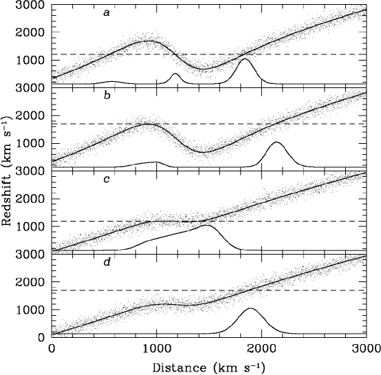
Figure 1: The effects of triple-valued or flat zones. The S-shaped curves show the relation between redshift and distance along two lines of sight to a cluster. (a) A galaxy with a redshift of 1200 km s^-1 can lie at three distinct distances. When the small-scale noise inherent in any velocity field model, as indicated by the scattered points, is taken into account, the quantity $P(r|cz),$ shown as the three-peaked curve at the bottom, gets smoothed out. (b) A galaxy at 1700 km s^-1 along the same line of sight intersects the redshift-distance curve at only one point, but comes close enough to it elsewhere to give a second peak to the $P(r|cz)$ curve. (c) Further from the cluster, the redshift-distance curve becomes flat, giving a broad peak to $P(r|cz)$. (d) At a redshift sufficiently far from a triple-valued zone, $P(r|cz)$ has only one narrow peak.

Two final details deserve brief mention. First, the integrals over $m$ and $\eta$ that appear in the denominators of Eqs. (11) and (12) may be done analytically for the case of “one-catalog selection” studied by Willick (1994, § 4.1), which indeed applies for the samples used in this paper (Willick et al. 1996). The numerical integrations required to evaluate Eqs. (11) and (12) are thus one-dimensional only. Second, as noted above, the velocity width distribution function $\phi(\eta)$ drops out of Eq. (11), but the luminosity function $\Phi(M)$ does not drop out of Eq. (12). Thus, inverse VELMOD requires that we model the luminosity function of TF galaxies. This is an annoyance at best, and could introduce biases, if we model it incorrectly, at worst. We have thus chosen to implement only forward VELMOD in this paper. On the other hand, inverse VELMOD enjoys the virtue that inverse Method II approaches do generally: to the degree that the selection function $S$ is independent of $\eta$ and $r,$ it drops out of Eq. (12). In a future paper, we will apply the small-$\sigma_{v}$ approximation to VELMOD for more extensive samples to larger distances. For that analysis the inverse approach will be used as well.

2.2.3 Implementation of VELMOD

The probability distribution $P(m|\eta,cz)$ (Eq. 11) is dependent on a number of free parameters, most importantly $\beta_{I}$. However, because $\beta_{I}$ enters at an earlier stage—in the reconstruction of the underlying density and velocity fields from IRAS (Appendix A)—it is on a different footing from other parameters. Thus, rather than treating $\beta_{I}$ as a continuous free parameter, VELMOD is run sequentially for the ten discrete values $\beta_{I}=0.1,\ldots,1.0$ for the real data, and for the nine discrete values $\beta_{I}=0.6,\ldots,1.4$ for the mock catalog data (§ 3). For each $\beta_{I},$ probability is maximized (${\cal L}_{{\rm forw}}$ is minimized) with respect to the remaining free parameters. These parameters are:

1. The TF parameters $A$, $b,$ and $\sigma_{{\rm TF}}$ for each sample in the analysis. Here we limit the analysis to the Mathewson et al. (1992; MAT) and Aaronson et al. (1982a; A82) samples, as we discuss in § 4.1. Thus, there are a total of 6 TF parameters that are varied. Note that the TF scatters are not simply calculated a posteriori. The statistic ${\cal L}_{{\rm forw}}$ depends on their values and they are varied to minimize it.

2. The small-scale velocity dispersion $\sigma_{v}.$ The quantities $\sigma_{v}$ and $\sigma_{{\rm TF}}$ can trade off to a certain extent (cf. Eq. 15). However, their relative importance depends on distance. Sufficiently nearby ($\lower 2.15277pt\hbox{$\,\buildrel<\over{\sim}\,$}1000\ {\rm km}\,{\rm s}^{-1}$), $\sigma_{v}$ is as large or a larger source of error than the TF scatter itself. Thus it is determined in this local region. Beyond $\sim\,$2000 km s^-1, the TF scatter dominates the error, and it is determined at these distances. Because the samples populate a range of distances, the two can be determined separately, with relatively little covariance.

3. We also allow for a Local Group random velocity vector ${\bf w}_{{\rm LG}}.$ The IRAS peculiar velocity predictions are given in the Local Group frame (Eq. 30). That is, the computed Local Group peculiar velocity vector has been subtracted from all other peculiar velocities. However, just as we expect all external galaxies to have a noisy as well as a systematic component to their peculiar velocity, so we must expect the Local Group to have one as well, especially considering the uncertainties in the conversion from heliocentric to Local Group frame. We allow for this by writing $u(r)=u_{\sl IRAS\/}(r)-{\bf w}_{{\rm LG}}\cdot\hat{\bf r},$ where $u_{\sl IRAS\/}(r)$ is given as described in Appendix A, and the three Cartesian components of ${\bf w}_{{\rm LG}}$ are varied in each VELMOD run at a given $\beta_{I}.$ We note briefly that this procedure is self-consistent only as long as $|{\bf w}_{{\rm LG}}|$ is at most comparable to $\sigma_{v}.$ In practice, we will find that for $\beta_{I}$ near its best value, the amplitude of ${\bf w}_{{\rm LG}}$ is trivially small.

4. Finally, we allow for the existence of a quadrupole velocity component that is not included in the IRAS velocity field. The justification for such a velocity component will be discussed in § 4.4 and Appendix B. The quadrupole is specified by five independent parameters, although we will not take them as free in the final analysis (we discuss this further in § 4.4).

Thus there are $3\times 2+1+3=10$ free parameters that are varied for any given value of $\beta_{I},$ when the quadrupole is held fixed. Thus, for any value of $\beta_{I},$ we give the data the fairest chance it possibly has to fit the IRAS model. In particular, the TF relations for the two separate samples used are not “precalibrated” in any way. This ensures that TF calibration in no way prejudices the value of $\beta_{I}$ we derive.

3 Tests With Simulated Galaxy Catalogs

In this section, we test the VELMOD method on simulated data sets. Kolatt et al. (1996) have produced simulated catalogs that mimic the properties of both the IRAS redshift survey and the Mark III samples. We briefly review the salient points here.

The mass density distribution of the simulated universe is based on the distribution of IRAS galaxies in the real universe. This was achieved by, first, taking the present redshift distribution of IRAS galaxies and solving for a 500 km s^-1 smoothed real-space distribution via an iterative procedure that applies nonlinear corrections and a power-preserving filter (Sigad et al. 1997). The smoothed, filtered IRAS density field was then “taken back in time” using the Zel’dovich-Bernoulli algorithm of Nusser & Dekel (1992) to obtain the linear initial density field. The method of constrained realization (Hoffman & Ribak 1991; Ganon & Hoffman 1993) was used to restore small-scale power down to galactic scales. The resulting initial conditions were then evolved forward as an $\Omega=1$ $N$-body simulation using the PM code of Gelb & Bertschinger (1994). The present-day density field resulting from this procedure is displayed in Figure 6 of Kolatt et al. (1996).

We generated a suite of 20 mock Mark III and mock IRAS catalogs from this simulated universe. Each mock Mark III TF sample was constructed to mimic the distribution on the sky and in redshift space of the corresponding real sample, and the TF relations and scatters of the mock samples were chosen to be similar to the observed ones. The mock TF samples were subject to selection criteria similar to those imposed on the real samples. The mock IRAS redshift catalogs were generated so as to resemble the actual IRAS 1.2 Jy redshift survey. They have the true IRAS selection and luminosity functions applied, and lack data in the IRAS excluded zones (cf. Strauss et al. 1990). These data were then put through exactly the same code to derive peculiar velocity and density fields as is used for the real data (Appendix A). To simplify interpretation of the mock catalog tests, the mock IRAS galaxies were generated with probability proportional to the mass density itself. Thus, the mock IRAS galaxies are unbiased relative to the mass; i.e., for the mock catalogs $b_{I}=1,$ and therefore the true value of $\beta_{I}$ for the simulated data is unity.

3.1 Accuracy of the $\beta$ Determination

The IRAS velocity field reconstructions may be produced using a variety of smoothing scales, and we have used 300 and 500 km s^-1 Gaussian smoothing. We found, however, that at 500 km s^-1 smoothing VELMOD returned a mean $\beta_{I}$ biased high by $\sim\,$20%; the predicted peculiar velocities were too small, and a too-large $\beta_{I}$ was needed to compensate. Our discussion from this point on will refer to 300 km s^-1 smoothing, which, as we now describe, we found to yield correct peculiar velocities and an unbiased estimate of $\beta_{I}.$

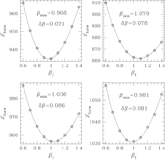
Figure 2: Plots of the likelihood statistic, ${\cal L}_{{\rm forw}},$ versus $\beta_{I}$ for VELMOD runs using four of the mock catalogs. (The true value of $\beta_{I}$ for the mock catalogs is unity, as discussed in the text.) Also indicated on the plots are $\beta_{{\rm min}},$ the maximum likelihood values for $\beta_{I},$ and the average of its two one-sided errors $\delta\beta_{\pm}.$ The solid lines drawn through the points are the cubic fits used to determine $\beta_{{\rm min}}$ and $\delta\beta_{\pm}.$

VELMOD was run on the 20 mock catalogs, and likelihood (${\cal L}_{{\rm forw}}$) versus $\beta_{I}$ curves were generated for each. As with the real data (§ 4), we used only the A82 and MAT TF samples; we limited the analysis to $cz\leq 3500\ {\rm km}\,{\rm s}^{-1}$. The curves were fitted with a cubic equation of the form

$${\cal L}={\cal L}_{0}+q\,(\beta_{I}-\beta_{{\rm min}})^{2}+p\,(\beta_{I}-\beta_{{\rm min}})^{3}$$ (17)

to determine $\beta_{{\rm min}},$ the value of $\beta_{I}$ for which ${\cal L}_{{\rm forw}}$ is minimized. This is the maximum likelihood value of $\beta_{I}.$ Four representative ${\cal L}_{{\rm forw}}$ versus $\beta_{I}$ plots are shown in Figure 2, along with the cubic fits. We estimate the $1\,\sigma$ errors $\delta\beta_{\pm}$ in our maximum likelihood estimate by noting the values $\beta\pm\delta\beta_{\pm}$ at which ${\cal L}={\cal L}_{0}+1.$ Given the presence of the cubic term in Eq. (17), this is not necessarily rigorous, but we can test our errors by defining the $\chi^{2}$-like statistic

$$\chi^{2}=\sum\,(\beta_{{\rm min}}-1)^{2}/\delta\beta_{\pm}^{2}\,,$$ (18)

where $\delta\beta_{+}$ was used if $\beta_{{\rm min}}\leq 1,$ and $\delta\beta_{-}$ was used if $\beta_{{\rm min}}>1.$ For the 20 mock catalogs, it was found that $\chi^{2}=21.2.$ Thus, our tests were consistent with the statement that the error estimates obtained from the change in the likelihood statistic near its minimum are true 1 $\sigma$ error estimates. Although we formally derive two-sided error bars, the upper and lower errors differ little, and when we discuss the real data (§ 4) we will give only the average of the two. The weighted mean value of $\beta_{{\rm min}}$ over the mock catalogs was $0.984$, with an error in the mean of $\sim 0.08/\sqrt{20}=0.017.$ Thus, the mean $\beta_{{\rm min}}$ is within $\sim 1\,\sigma$ from the true answer. We conclude that there is no statistically significant bias in the VELMOD estimate of $\beta_{I}.$ The results of this and other tests we carried out using the mock catalogs are summarized in Table 1.

3.2 Accuracy of the Determination of $\sigma_{v}$ and ${\bf w}_{{\rm LG}}$

The mock catalogs also enable us to determine the reliability of the small-scale velocity dispersion $\sigma_{v}$ derived from VELMOD. This quantity may be viewed as the quadrature sum of true velocity noise ($\sigma_{v}^{n}$) and IRAS velocity prediction errors ($\sigma_{v}^{I}$) resulting from shot-noise and imperfectly modeled nonlinearities. (For the real data, there is an additional contribution from redshift measurement errors, which are zero in the mock catalog.) We can measure both $\sigma_{v}^{n}$ and $\sigma_{v}^{I}$ directly from the mock catalogs. To measure velocity noise, we determined $\sigma_{u},$ the rms value of pair velocity differences $cz({\bf r}_{i})-cz({\bf r}_{j})$ of mock catalog TF galaxies within 3500 km s^-1 outside of the mock Virgo core, for $|{\bf r}_{i}-{\bf r}_{j}|\leq r_{{\rm max}}.$ We found $\sigma_{u}$ to be insensitive to the precise value of $r_{{\rm max}}$ provided it was $\lower 2.15277pt\hbox{$\,\buildrel<\over{\sim}\,$}150\ {\rm km}\,{\rm s}^{-1},$ implying that we are not including the gradient of the true velocity field on these scales. Taking $r_{{\rm max}}=150\ {\rm km}\,{\rm s}^{-1},$ we found $\sigma_{u}=71\ {\rm km}\,{\rm s}^{-1},$ corresponding to $\sigma_{v}^{n}=\sigma_{u}/\sqrt{2}=50\ {\rm km}\,{\rm s}^{-1}.$ This value is so small because the PM code does not properly model particle-particle interactions on small scales.

We measured the IRAS prediction errors $\sigma_{v}^{I}$ as follows. For each mock TF particle (again, within 3500 km s^-1 and outside the mock Virgo core), we computed an IRAS predicted redshift $cz^{I}_{i}=r_{i}+u(r_{i})+fr_{i}-{\bf w}_{{\rm LG}}\cdot{\hat{\bf n}}_{i},$ where $r_{i}$ was the true distance of the object, $u(r_{i})$ was the IRAS-predicted radial peculiar velocity in the Local Group frame (for $\beta_{I}=1$), $f$ was a zero-point error in the IRAS model (cf. § 3.3), and ${\bf w}_{{\rm LG}}$ was the mock Local Group peculiar velocity, which (just as in the real data) is not known precisely and was also treated as a free parameter. We then minimized the mean squared difference between $cz^{I}_{i}$ and the actual redshifts $cz_{i}$ over the entire TF sample with respect to $f$ and ${\bf w}_{{\rm LG}}.$ The rms value of $(cz_{i}-cz^{I}_{i})$ at the minimum was then our estimate of the quadrature sum of IRAS prediction error and true velocity noise, which we found to be $98\pm 2\ {\rm km}\,{\rm s}^{-1}$ after averaging over the 20 mock catalogs. Subtracting off the small value of $\sigma_{v}^{n}$ found above, we obtain $\sigma_{v}^{I}\simeq 84\ {\rm km}\,{\rm s}^{-1}.$ This surprisingly small value is indicative of the high accuracy of the IRAS predictions for nearby galaxies not in high density environments.

The value $\sigma_{v}=98\ {\rm km}\,{\rm s}^{-1}$ is somewhat smaller than the real universe value of $\sigma_{v}=125\ {\rm km}\,{\rm s}^{-1}$ (§ 4.5). Because we wanted the mock catalogs to reflect the errors in the real data, we added artificial velocity noise of $110\ {\rm km}\,{\rm s}^{-1}$ to the redshift of each mock TF galaxy before applying the VELMOD algorithm, increasing $\sigma_{v}$ to $147\ {\rm km}\,{\rm s}^{-1}.$ The mean value of $\sigma_{v}$ from the VELMOD runs on the 20 mock catalogs was ${\left\langle\sigma_{v}\right\rangle}=148.7\ \pm 4.6\ {\rm km}\,{\rm s}^{-1},$ in excellent agreement with the expected value. We conclude that VELMOD produces an unbiased estimate of the $\sigma_{v},$ just as it does of $\beta_{I}.$ The rms error in the determination of $\sigma_{v}$ from a single realization is $\sim 20\ {\rm km}\,{\rm s}^{-1}$.

The calculation in which we minimized $(cz_{i}-cz^{I}_{i})^{2}$ also yielded estimates of the Cartesian components of Local Group random velocity vector ${\bf w}_{{\rm LG}}.$ Their mean values over 20 mock catalogs is given in Table 1, together with the corresponding mean values returned from VELMOD over the 20 mock catalog runs. The two are in impressive agreement. These values reflect an offset between the CMB to LG transformation assigned to the simulation and the average value of ${\bf w}_{{\rm LG}}$ assigned by the mock IRAS reconstruction for $\beta_{I}=1$. We conclude that VELMOD properly measures the Cartesian components of ${\bf w}_{{\rm LG}}$ to within $\sim\,$50 km s^-1 accuracy per mock catalog.

3.3 The TF Parameters Obtained from VELMOD

The mock catalogs also enable us to test the accuracy of the TF parameters determined from the likelihood maximization procedure. The comparison of input and output values is given in Table 1. The results for the TF slope and scatter are consistent with the statement that VELMOD returns unbiased values of these TF parameters for each of the two samples. The fact that the TF scatters and $\sigma_{v}$ are unbiased means that VELMOD correctly measures the overall variance in peculiar velocity predictions.

The TF zero points returned by VELMOD are systematically in error by 2–3 standard deviations. This can be traced to a bias in the IRAS-predicted peculiar velocities; the mean value of the quantity $f$ in § 3.2 over 20 realizations was $0.018\pm 0.007$. This bias makes the IRAS-predicted distances $d_{\sl IRAS\/}\simeq cz-u_{\sl IRAS\/}$ too large by a factor of $1.018,$ or $\sim\,$0.04 mag. To bring the TF and IRAS distances into agreement, the TF zero points must decrease by this amount, which in fact they do (cf. Table 1). Thus, VELMOD determines the TF zero points in such a way as to compensate for a small systematic error in the IRAS predictions. We expect such an error to be present in the real data as well, but it will be completely absorbed into the TF zero points, and our derived value of $\beta_{I}$ will be unaffected.

3.4 Properties of the VELMOD Likelihood

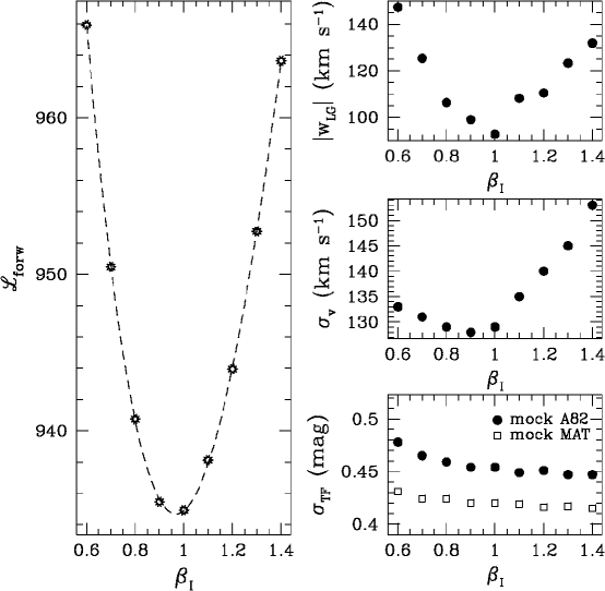
Figure 3: Some of the parameters obtained from running VELMOD on a single mock catalog. The left hand panel shows the likelihood statistic along with the cubic fit used to determine its minimum. The right hand panels show the amplitude of the Local Group random velocity vector, the velocity noise $\sigma_{v},$ and the TF scatters for the mock A82 and mock MAT samples. Note that the Local Group velocity vector has its minimum amplitude for $\beta_{I}\simeq 1.$ Note also that the TF scatters do not track the likelihood curve, primarily because the velocity noise $\sigma_{v}$ also measures the inaccuracy of the fit. This demonstrates that minimizing TF scatter is not equivalent to maximizing likelihood, as it is for standard Method II.

The mock catalogs may also be used to illustrate some important features of the VELMOD analysis. An example of these is shown in Figure 3. The left hand panel shows ${\cal L}_{{\rm forw}}$ versus $\beta_{I}$ for one of the 20 catalogs. The right hand panels show how three other quantities vary with $\beta_{I}$ in the same VELMOD run: the amplitude of the LG random velocity ${\bf w}_{{\rm LG}}$ (top panel), the velocity noise $\sigma_{v},$ and the TF scatter $\sigma_{{\rm TF}}$ for each of the two mock TF samples (A82 and MAT) considered (bottom panel). Note first that the amplitude of the LG velocity vector is minimized near the true value of $\beta_{I}.$ This was generally seen in the mock catalogs; it reflects the fact that the fits at the wrong values of $\beta_{I}$ try to compensate for wrong peculiar velocity predictions with Local Group motion. If ${\bf w}_{{\rm LG}}$ were held fixed at its maximum likelihood value, or set equal to zero, the ${\cal L}_{{\rm forw}}$ versus $\beta_{I}$ curves would have sharper minima and the $\beta$-uncertainty would be reduced (cf. § 4.5). Unfortunately, we cannot do this for the real universe because we do not know ${\bf w}_{{\rm LG}}$ a priori. Nevertheless, there we will find similar behavior; ${\bf w}_{{\rm LG}}$ has a minimum near the best-fit value of $\beta_{I}$ for the real universe.

The figure also shows that $\sigma_{v}$ is a weak function of $\beta_{I}$, but goes to a minimum at $\beta_{I}\approx 1$. Its value at the minimum for this realization is 127 km s^-1, within $1\,\sigma$ of the correct value (Table 1). The $\sigma_{{\rm TF}}$ are also weak functions of $\beta_{I}$, but are in good agreement with the input values near the maximum likelihood values of $\beta_{I}.$ Most importantly, the figure demonstrates that maximizing likelihood does not necessarily correspond to minimizing TF scatter, as we argued in § 2.2.2. The TF scatters in fact decrease monotonically with increasing $\beta_{I}.$ As they do, $\sigma_{v}$ increases to compensate. However, one cannot simply minimize $\sigma_{{\rm TF}},$ or even a simple combination of $\sigma_{{\rm TF}}$ and $\sigma_{v},$ to obtain an unbiased $\beta_{I}.$ One must instead maximize likelihood as defined in § 2.2.1.

4 Application to the Mark III Catalog Data

4.1 Sample Selection

To apply VELMOD to the real TF data, we needed first to identify a suitable subsample of the Mark III catalog. As discussed in § 2.2.2, we elected to restrict the TF sample to $cz_{{\rm LG}}\leq 3000\ {\rm km}\,{\rm s}^{-1}$, where here and throughout, we correct heliocentric redshifts to the Local Group frame following Yahil, Tammann, & Sandage (1977). We thus use the Aaronson et al. (1982a; A82) and Mathewson et al. (1992; MAT) TF samples, which are rich in local galaxies, restricted to this redshift interval. The two cluster samples in the Mark III catalog, HMCL and W91CL, contain only clusters at greater redshifts and thus are not used here. Finally, only a small fraction of the W91PP and CF samples is found at $cz_{{\rm LG}}\leq 3000\ {\rm km}\,{\rm s}^{-1}$ ($\sim\,$2% of W91PP, $\sim\,$15% of CF). This small number of additional galaxies was not worth the additional 6 free parameters that would be required for the likelihood maximization procedure (§ 2).

We made several further cuts on the data, as follows:

1. An RC3 $B$-magnitude limit of $m_{B}=14.0$ mag was adopted for A82. As discussed by Willick et al. (1996), A82 galaxies within 3000 km s^-1, and subject to this magnitude limit, are well described by the “one-catalog” selection function of Willick (1994) that enters into the likelihood equations (§ 2).

2. An ESO $B$-band diameter limit of $d_{{\rm ESO}}=1.6$ arcminute was adopted for MAT. As discussed by Willick et al. (1996), this allows the MAT subsample to be described by the one-catalog selection function of Willick (1994).

3. Only galaxies with axial ratios $\log(a/b)\geq 0.1$ were included. This cut, corresponding to an inclination limit of $i\geq 38^{\circ}\,$ (Willick et al. 1997), reduces TF scatter due to velocity width errors.

4. Galaxies with $\eta<-0.45$ (rotation velocities less than about 55 km s^-1) were excluded. In practice, this criterion applied only to the MAT sample, which contains numerous very low-linewidth galaxies. The need for excluding such objects was discussed by Willick et al. (1996).

5. Two objects within the Local Group, defined as having raw forward TF distances $<100\ {\rm km}\,{\rm s}^{-1},$ were excluded. No lower bound was placed on the redshifts of sample objects, however.

This left a sample of 856 A82 and MAT galaxies. As discussed by Willick et al. (1996, 1997), real samples exhibit a mainly Gaussian distribution of TF residuals, but with an admixture of a few percent of non-Gaussian outliers. We excluded eighteen additional galaxies (4 in A82, 14 in MAT), or $\sim\,$2% of our sample, because of their extremely large residuals from the TF relation. Finally, then, 838 galaxies, 300 in A82 and 538 in MAT, were used in the VELMOD analysis. Of these, 53 are objects found in both samples (though with different raw data), and thus are used twice in the analysis.

4.2 Velocity-Width Dependence of the TF Scatter

It has been noted by a number of authors (Federspiel, Sandage, & Tammann 1994; Willick et al. 1997; Giovanelli et al. 1997) that $\sigma_{{\rm TF}}$ exhibits a velocity-width (or, equivalently, a luminosity) dependence: luminous, rapidly rotating galaxies have smaller TF scatter than faint, slowly rotating ones. Willick et al. (1997) showed that this effect could be parameterized by $\sigma_{{\rm TF}}(\eta)=\sigma_{0}-g\eta,$ with different values of $\sigma_{0}$ (the scatter for a typical, $\eta=0$, galaxy) and $g$ for each sample. For the MAT sample, they found $g=0.33,$ while for A82 they found $g=0.14.$ In the VELMOD analysis, we treated $\sigma_{0}$ as a free parameter for both samples, but fixed the values of $g$ to the Willick et al. (1997) values. For the remainder of this paper, when we refer to $\sigma_{{\rm TF}}$ we are actually referring to the $\sigma_{0}$ for the respective samples. We note that a significant likelihood increase was achieved by adopting this variable TF scatter, but that the derived value of $\beta_{I}$ was essentially unchanged. The mock catalogs were generated and analyzed with $g=0$.

4.3 Treatment of Virgo

To simplify the analysis, we have taken the small-scale velocity noise, $\sigma_{v},$ to be independent of position. Clearly, this assumption must fail in the immediate vicinity of a rich cluster. The Virgo cluster is the only rich cluster within 3000 km s^-1. Thus, we must artificially “cool down” the galaxies near Virgo. We do so as follows: if a galaxy lies within 10${}^{\circ}\,$ of the Virgo core (taken to be $l=283.78^{\circ}\,,$ $b=74.49^{\circ}\,$) on the sky, within 1500 km s^-1 of its mean Local Group redshift (taken to be $1035.1\ {\rm km}\,{\rm s}^{-1},$ following Huchra 1985), and has a raw TF distance from Willick et al. (1997) between 800 and 2100 km s^-1, its Local Group redshift is set to the mean Virgo value. Twenty objects used in the VELMOD analysis meet these criteria. We similarly collapsed mock Mark III objects associated with the Virgo cluster in the mock catalogs.

4.4 Implementation of a Quadrupole Flow

In the discussion of VELMOD in § 2, it was assumed that the IRAS-predicted velocity field, for the correct value of $\beta_{I},$ is as good a model as can be obtained. However, there can be additional contributions to the local flow field from structures beyond the volume surveyed ($R\leq 12,800\ {\rm km}\,{\rm s}^{-1}$), as well as from shot noise- and Wiener-filter-induced differences between the true and derived density fields beyond 3000 km s^-1 but within the IRAS volume (cf. Appendix B).

Fortunately, the nature of this contribution is such that we can straightforwardly model its general form, and thus treat it as a quasi-free parameter (see below) in the VELMOD fit. Let us write the error in the IRAS-predicted velocity field due to incompletely sampled fluctuations as ${\bf v}_{{\rm err}}({\bf r}).$ Because the total peculiar velocity field, ${\bf v}+{\bf v}_{{\rm err}}$ must satisfy Eq. (4), and because ${\bf v}$ does so by construction (Eq. 3), it follows that ${\bf v}_{{\rm err}}$ must have zero divergence. Moreover, if we suppose that ${\bf v}_{{\rm err}}$ corresponds to the growing mode of the linear peculiar velocity field, it must have zero curl as well. These properties will be satisfied if ${\bf v}_{{\rm err}}$ is given by the gradient of a velocity potential $\phi$ that satisfies Laplace’s equation. Such a potential may be expanded in a multipole series, each term of which vanishes at the origin (where, by construction, ${\bf v}_{{\rm err}}$ must itself vanish).

The leading term in the resulting expansion of ${\bf v}_{{\rm err}}$ is a monopole, ${\bf v}_{{\rm err}}^{(0)}({\bf r})=A{\bf r},$ or Hubble flow-like term. However, such a term is degenerate with the zero point of the TF relation (§ 3.3), and is thus undetectable. The next term in the expansion is a dipole, ${\bf v}_{{\rm err}}^{(1)}={\bf B},$ or bulk flow independent of position. Like the monopole term, however, the dipole term is undetectable, because we work in the frame of the Local Group. Whatever bulk flow is generated by distant density fluctuations is shared by the Local Group as well. The leading term in the expansion of ${\bf v}_{{\rm err}}({\bf r})$ to which our method is sensitive is therefore a quadrupole term. Such a term represents the tidal field of mass density fluctuations not traced by the IRAS galaxies. We may write the quadrupole velocity component as

$${\bf v}_{Q}({\bf r})={\cal V}_{Q}\,{\bf r},$$ (19)

where ${\cal V}_{Q}$ is a $3\times 3$ matrix. In order for both the divergence and curl of ${\bf v}_{Q}({\bf r})$ to vanish, ${\cal V}_{Q}$ must be a traceless, symmetric matrix. Consequently, it has only five independent elements, two diagonal and three off-diagonal.

We could allow for the presence of such a quadrupole in VELMOD by treating these five elements as free parameters. However, this is a dangerous procedure, because the modeled quadrupole would then have the freedom to fit the quadrupole already present in the IRAS velocity field, which is generated by observed density fluctuations. We wish to allow for the external quadrupole, but we do not want it to fit the $\beta$-dependent quadrupolar component of the IRAS-predicted velocity field. In other words, we want the external quadrupole to be that required for the true value of $\beta_{I},$ which we do not know a priori, rather than the “best fit” value at any given $\beta_{I}.$ This problem would indeed be very serious if inclusion of the quadrupole made a large difference in the derived value of $\beta_{I}.$ Fortunately, however, it does not. As we show below, we obtain a maximum likelihood value $\beta_{I}=0.56$ when the quadrupole is not modeled. When we treat all five components of the quadrupole as free parameters for each $\beta_{I},$ we obtain $\beta_{I}=0.47.$ Because the best-fit quadrupole is relatively insensitive to $\beta_{I},$ we can estimate the external quadrupole by averaging the fitted values of the five independent components obtained for $\beta_{I}=0.1,0.2,\ldots,1.0.$ In this way, we “project out” the $\beta_{I}$-independent part of the quadrupole. In our final VELMOD run, we use this average external quadrupole at each value of $\beta_{I}.$ Throughout, we ignore the very small effect that this quadrupole might have on the derived IRAS density field.

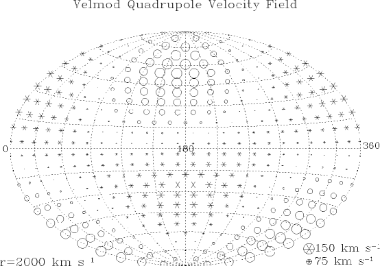
Figure 4: The external quadrupolar velocity field used in the VELMOD analysis, plotted in Galactic coordinates. Open symbols indicate negative radial velocities, stars positive radial velocities. The amplitude of the quadrupole is shown for a distance $r=2000\ {\rm km}\,{\rm s}^{-1}.$ As indicated by Eq. (19), the quadrupole flow increases linearly with distance at a given position on the sky. The maximum amplitude of the quadrupole at this distance is 147 km s^-1, which occurs at $l\simeq 165^{\circ}\,,$ $b\simeq 55^{\circ}\,,$ as well as on the opposite side of the sky.

In Figure 4, this quadrupole field is plotted on the sky in Galactic coordinates for a distance of 2000 km s^-1. The inflow due to the quadrupole, which occurs near the Galactic poles, is of greater amplitude than the outflow, which occurs at low Galactic latitude. The quadrupole reaches its maximum amplitude at $l\simeq 165^{\circ}\,,$ $b\simeq 55^{\circ}\,,$ in the direction of the Ursa Major cluster, as well as on the opposite side of the sky. In § 5, when we plot VELMOD residuals on the sky with and without the quadrupole, the need for the quadrupole field shown in Figure 4 will become clear. Indeed, we will show in § 5 that the VELMOD fit is statistically acceptable only when the quadrupole is included. Table Maximum-Likelihood Comparisons of Tully-Fisher and Redshift Data: Constraints on $\Omega$ and Biasing tabulates the numerical values of the independent elements of ${\cal V}_{Q}$ that generate this flow. The rms value of this quadrupole over the sky is 3.3%, pleasingly close to the value we expect from theoretical considerations (Appendix B).

When both the quadrupole and the Local Group random velocity vector are modeled, the radial peculiar velocity $u(r)$ that enters into the likelihood analysis (see Eq. 9) is given by

$$u(r)=\left({\bf v}_{\sl IRAS\/}({\bf r})+{\cal V}_{Q}{\bf r}-{\bf w}_{{\rm LG}}\right)\cdot\hat{\bf r}\,.$$ (20)

We emphasize again that while the three components of the Local Group random velocity ${\bf w}_{{\rm LG}}$ are treated as free parameters in VELMOD, the five independent parameters of ${\cal V}_{Q}$ are not, with the exception of a single run we used to obtain and then average their fitted values at each $\beta_{I}.$ In the final run, from which we derive the estimate of $\beta_{I}$ quoted in the Abstract, the quadrupole velocity field shown in Figure 4 was used at each value of $\beta_{I}.$

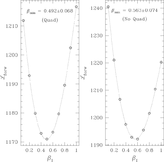
Figure 5: The VELMOD likelihood statistic, ${\cal L}_{{\rm forw}}$ (Eq. 13), plotted as a function of $\beta_{I}$ for the real data. In the left hand plot, an external quadrupole is modeled, as described in the text. In the right hand plot, no external quadrupole is included in the velocity field. Cubic fits to the likelihood points are shown as dotted lines. The minima of the fitted curves, $\beta_{{\rm min}},$ are the maximum likelihood estimates of $\beta_{I}$ in each case. Note the very different values of the vertical axes of the two plots; this indicates the large increase in formal likelihood when the quadrupole is included.

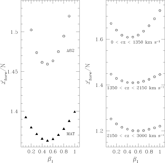
Figure 6: Breakdown of the VELMOD likelihood statistic among subsamples. The left hand panel plots likelihood per point versus $\beta_{I}$ for the A82 and MAT samples individually. The right hand panel plots likelihood per point versus $\beta_{I}$ for three different redshift intervals containing roughly the same number of objects. In each case, the minimum occurs within $\sim\,$0.1 in $\beta_{I}$ of the global minimum in ${\cal L}_{{\rm forw}}$ at $\beta_{I}=0.492.$

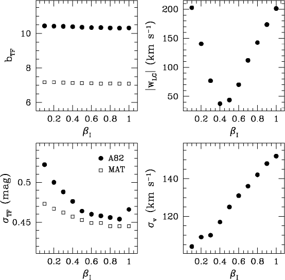
Figure 7: Left hand panels: the TF slopes (top) and scatters (bottom), for the A82 and MAT samples, derived from VELMOD as a function of $\beta_{I}.$ Right hand panels: the amplitude of the Local Group random velocity vector (top) and the velocity noise $\sigma_{v}$ (bottom) derived from VELMOD as a function of $\beta_{I}.$ All plots correspond to the run in which the quadrupole was modeled.

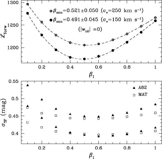
Figure 8: Top panel: The VELMOD likelihood statistic ${\cal L}_{{\rm forw}}$ as a function of $\beta_{I}$ for a two runs in which the Local Group velocity vector was forced to vanish, and the velocity noise parameter $\sigma_{v}$ was held fixed at 150 and 250 km s^-1. Although the formal likelihoods of the fit are worse than that of the full fit (compare with Figure 5), particularly for $\sigma_{v}=250\ {\rm km}\,{\rm s}^{-1},$ the maximum likelihood estimates of $\beta_{I}$ are nearly unchanged. Bottom panel: variation in the TF scatters $\sigma_{{\rm TF}},$ for the A82 and MAT samples, as a function of $\beta_{I}$ for these VELMOD runs. The larger values correspond to the $\sigma_{v}=150\ {\rm km}\,{\rm s}^{-1}$ run. Note that the minimum derived TF scatters do not necessarily correspond to maximum likelihood; see text for further details.

4.5 Results

The outcome of applying VELMOD to the A82+MAT subsample described above is presented in Figure 5. The VELMOD likelihood curves are shown both with and without the external quadrupole included. The formal likelihood is vastly improved when the quadrupole is included in the fit: since the likelihood statistic ${\cal L}_{{\rm forw}}$ is defined as $-2\ln\left[P({\rm data}|\beta)\right],$ the $\sim\,$20 point reduction in the minimum of ${\cal L}_{{\rm forw}}$, minus the five extra degrees of freedom when the quadrupole is modeled corresponds to a probability increase of a factor $\sim e^{7.5}\simeq 2000.$ The improvement in formal likelihood through the addition of the quadrupole is so pronounced that we take the maximum likelihood value of $\beta_{I}$ from that fit, $0.492\pm 0.068,$ as our best estimate. However, the maximum likelihood estimate of $\beta_{I}$ when the quadrupole is neglected, $0.563\pm 0.074,$ differs from our best value at only the 1-$\sigma$ level. While the quadrupole is important, it does not qualitatively affect our conclusions about the likely value of $\beta_{I}.$

We can make several additional tests of the robustness of our results. Figure 6 shows how the likelihoods per object break down for fits to different cuts on the sample; see also Table Maximum-Likelihood Comparisons of Tully-Fisher and Redshift Data: Constraints on $\Omega$ and Biasing. The left hand panel plots ${\cal L}_{{\rm forw}}/N$ versus $\beta_{I}$ for the A82 and MAT samples separately, where $N=300$ for A82 and $N=538$ for MAT. Cubic fits to the individual sample likelihoods yield $\beta_{I}=0.489\pm 0.084$ and $0.498\pm 0.107$ for A82 and MAT respectively. This agreement is remarkable, given that there are only 53 galaxies in common between the two samples. Note that the $\beta$-uncertainty is larger for the MAT sample, even though it contains nearly twice as many objects as the A82 sample. This is because the MAT objects typically lie at larger distances than do A82 objects, a property of the likelihood fit we now illustrate.

The right hand panel of Figure 6 plots ${\cal L}_{{\rm forw}}/N$ versus $\beta_{I}$ for three subsamples in different redshift ranges. As Table Maximum-Likelihood Comparisons of Tully-Fisher and Redshift Data: Constraints on $\Omega$ and Biasing shows, the agreement in the derived values of $\beta_{I}$ is quite good. Changing the specific redshift intervals used for this test does not significantly change the results. Note that the $\beta$-resolution decreases as one goes to higher redshift, despite the fact that there are nearly equal numbers of objects in each of the three redshift bins. This is because the likelihood is sensitive mainly to the fractional distance error in the IRAS prediction. Hence, nearby galaxies are more diagnostic of incorrect peculiar velocity predictions, and thus of $\beta_{I}.$

The fact that ${\cal L}_{{\rm forw}}/N$ decreases with redshift should not be interpreted as meaning that more distant objects are better fit by the velocity model. This decrease instead reflects a property of the VELMOD likelihood implicit in Eq. (15), which shows that the expectation value of ${\cal L}_{{\rm forw}}/N$ is $\sim 1+\ln(2\pi)+\ln\left[\sigma_{{\rm TF}}^{2}+\left(2.17\sigma_{v}/[w(1+u^{\prime}(w))]\right)^{2}\right],$ which increases with decreasing $cz$ in general. This effect will be particularly pronounced in flat zones ($u^{\prime}\sim-1$) in the redshift-distance relation, which are found in the Local Supercluster, which is why there is a marked difference between ${\cal L}_{{\rm forw}}/N$ for the A82 and MAT samples (the former preferentially populates the Local Supercluster region).

In Figure 7 we plot for the real data the same quantities plotted for a mock catalog in Figure 3, as well as the TF slopes. The slopes are extremely insensitive to $\beta_{I}.$ This indicates that the IRAS assigns low and high linewidth galaxies nearly same relative distances at all $\beta_{I}.$ Significantly, the amplitude of the fitted Local Group velocity vector is minimized near the maximum likelihood value of $\beta_{I}$, just as we saw with the mock catalog. This indicates once again that the fit attempts to compensate for a poor velocity field at very low and high $\beta_{I}$ by moving the Local Group. The mock catalogs showed us that the errors on the Cartesian components of ${\bf w}_{{\rm LG}}$ are of order 50 km s^-1(Table 1). Thus, the small value of $|{\bf w}_{{\rm LG}}|$ obtained from VELMOD indicates that the Yahil et al. (1977) transformation to the Local Group barycenter is correct to within $\sim\,$50 km s^-1, and that the Local Group has random velocity $\lower 2.15277pt\hbox{$\,\buildrel<\over{\sim}\,$}50\ {\rm km}\,{\rm s}^{-1}$ relative to the mean peculiar velocity field in its neighborhood.

The lower right panel of Figure 7 shows that $\sigma_{v}$ increases monotonically with $\beta_{I}.$ Its maximum likelihood value is 125 km s^-1. This is a remarkably small number, when one considers that it includes the effect not only of random velocity noise but also of IRAS prediction error. In particular, if our estimate of the IRAS-prediction errors derived from our mock catalog experiments (§ 3.2), $\sim\,$84 km s^-1, are roughly correct, our value for $\sigma_{v}$ implies that the true 1-dimensional velocity noise is $\lower 2.15277pt\hbox{$\,\buildrel<\over{\sim}\,$}100\ {\rm km}\,{\rm s}^{-1}.$ This result is consistent with past observations that the velocity field is “cold” (cf., Sandage 1986; Brown & Peebles 1987; Burstein 1990; Groth, Juszkiewicz, & Ostriker 1989; Strauss, Cen, & Ostriker 1993; Strauss, Ostriker, & Cen 1997). Finally, the lower left panel demonstrates again what was seen earlier with the mock catalogs (Figure 3), namely, that maximizing probability does not correspond to minimizing TF scatter. In large measure, this is because there is a tradeoff between the variance due to the velocity noise $\sigma_{v}$ and that due to the TF scatter. As $\beta_{I}$ approaches 1, $\sigma_{v}$ gets steadily larger; $\sigma_{{\rm TF}}$ gets correspondingly smaller, despite the fact that the high $\beta_{I}$ models are worse fits to the TF data. The TF scatters level out or rise only at $\beta_{I}\simeq 1.$

A final test of robustness involves eliminating the freedom in the VELMOD fit provided by the parameters ${\bf w}_{{\rm LG}}$ and $\sigma_{v}.$ One could argue that these parameters are like the quadrupole: they “are what they are,” and we should not allow them to absorb the fit inaccuracies at the wrong value of $\beta_{I}.$ To assess this, we carried out two VELMOD runs in which ${\bf w}_{{\rm LG}}$ was assumed to vanish identically. In the first run, we fixed the value of $\sigma_{v}$ at 150 km s^-1, and in the second at 250 km s^-1. The quadrupole was held fixed at its best fit value; the free parameters in this fit were limited to $\beta_{I}$ and the three TF parameters for each of the two samples. The results of this exercise are shown in Figure 8 and in Table Maximum-Likelihood Comparisons of Tully-Fisher and Redshift Data: Constraints on $\Omega$ and Biasing. The derived values of $\beta_{I}$ differ inconsequentially from our best estimate obtained from the full fit. This shows that allowing ourselves the freedom to fit both ${\bf w}_{{\rm LG}}$ and $\sigma_{v}$ does not materially affect the derived value of $\beta_{I}.$ The formal uncertainties in $\beta_{I}$ are much reduced relative to the full fit because formerly free parameters have been held fixed. For $\sigma_{v}=150\ {\rm km}\,{\rm s}^{-1}$ the formal likelihood is worse than for the full fit, but only at the $\sim 2\,\sigma$ level. This reflects the fact that $\sigma_{v}=150\ {\rm km}\,{\rm s}^{-1}$ and ${\bf w}_{{\rm LG}}=0$ themselves differ by only $\sim\,$$1\,\sigma$ from their maximum likelihood values, according to our error estimates from § 3.2. However, the formal likelihood for the $\sigma_{v}=250\ {\rm km}\,{\rm s}^{-1}$ run is considerably worse (by a factor of $\sim 10^{-7}$) than for the full fit. This shows that we rule out such a large $\sigma_{v}$ at high significance.

The bottom panel of Figure 8 shows the fitted values of $\sigma_{{\rm TF}}$ as a function of $\beta_{I}$ for each of the two values of $\sigma_{v}$ and for each of the two TF samples. The TF scatters now track the likelihood much better than they did in the full fit (bottom panel of Figure 7); with $\sigma_{v}$ fixed, maximizing likelihood is more nearly equivalent to minimizing TF scatter. However, they are still not the same thing: likelihood maximization occurs for $\beta_{I}\simeq 0.5,$ whereas TF scatter is minimized at $\beta_{I}\simeq 0.6.$ This is due to the nonlocal nature of the probability distribution described by Eq. (11) (cf. Figure 1). The likelihood of a given data point depends on the peculiar velocity and density fields all along the line of sight interval allowed by the TF and velocity dispersion probability factors, not merely on how close the TF-inferred and IRAS-predicted distances are to one another.

The bottom panel of Figure 8 also shows that the TF scatter one derives from VELMOD depends on the value of $\sigma_{v}.$ The full fit told us that IRAS errors plus true velocity noise amount to $\sim\,$125 km s^-1. The values of $\sigma_{{\rm TF}}$ obtained in the full fit (Table Maximum-Likelihood Comparisons of Tully-Fisher and Redshift Data: Constraints on $\Omega$ and Biasing) absorbed the remaining variance. Changing $\sigma_{v}$ to 150 km s^-1 reduces the TF scatters by about 0.01 mag. With $\sigma_{v}$ fixed at 250 km s^-1, however, we find 0.39 and 0.40 mag for the A82 and MAT TF scatters. While these latter values are certainly underestimates, the large changes demonstrate that it is very difficult to estimate $\sigma_{{\rm TF}}$ to high accuracy because of its covariance, however slight, velocity noise. This is one reason that it is inadvisable to use the value of $\sigma_{{\rm TF}}$ obtained from fitting TF data to peculiar velocity models as a measure of the goodness of fit. We return to this issue in § 5 below.

4.6 VELMOD Results using 500 km s^-1 Smoothing

In our mock catalog tests, we found that using 500 km s^-1 smoothing in the IRAS reconstruction resulted in $\sim\,$20% overestimates of $\beta_{I}$ (§ 3.1). However, because the mock catalog may not faithfully reproduce the dynamics of the real universe, it is useful to see how much $\beta_{I}$ changes for the real data when the 500 km s^-1-smoothed IRAS reconstructions are used. We carried out two such VELMOD runs, one with and one without the quadrupole. (We determined the quadrupole the same way as for the 300 km s^-1 smoothed reconstruction, and found that the two differ little.) The resulting maximum likelihood estimates of $\beta_{I}$ are listed in Table Maximum-Likelihood Comparisons of Tully-Fisher and Redshift Data: Constraints on $\Omega$ and Biasing. The larger smoothing results in an increase in $\beta_{I},$ as expected. However, the 500 km s^-1 result, $\beta_{I}=0.544\pm 0.071,$ is within $1\,\sigma$ of our favored result obtained at 300 km s^-1 smoothing. If we reduce this value by 20% in accord with the bias seen in the mock catalogs, we obtain $\beta_{I}=0.45\pm 0.07,$ also within $1\,\sigma$ of our preferred result. Our choice of a 300 km s^-1 smoothing scale is thus unlikely to have led us seriously astray, even if the mock catalogs are imperfect guides.

4.7 Consistency of the Mark III and VELMOD TF Relations

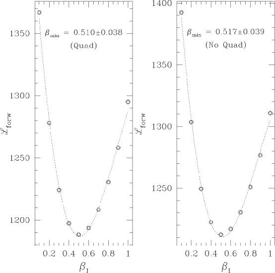
Figure 9: Same as Figure 5, except that the A82 and MAT TF parameters have been fixed at their Mark III catalog values. The extremely small formal error bars result from fixing the TF parameters and are unrealistic. The maximum likelihood values of $\beta_{I}$ differ negligibly from those obtained when the TF parameters are free.

In constructing the Mark III catalog, Willick et al. (1996, 1997) required that the TF distances for objects common to two or more samples agree in the mean. As noted above, VELMOD yields an independent TF calibration for each sample included in the analysis. As a further consistency check, we can ask whether the VELMOD TF calibrations for the A82 and MAT samples are also mutually consistent.

We compared A82 and MAT TF distances using the VELMOD TF relations for 75 objects common to the two samples. We limited the comparison to objects whose A82 versus MAT TF distance moduli differ by 0.8 mag or less. (Not all of these objects were part of the VELMOD analysis, as some did not meet the criteria outlined in § 4.1). We found that the VELMOD calibrations yield an average distance modulus difference (in the sense MAT$-$A82) $\left\langle\Delta\mu\right\rangle=-0.056\pm 0.046$ mag; the Mark III TF calibrations yield $\left\langle\Delta\mu\right\rangle=0.018\pm 0.046$ mag. The corresponding median distance modulus differences are $-0.015$ mag (VELMOD) and $0.035$ mag (Mark III). Thus, as measured by the criterion of generating mutually consistent TF distances among samples, VELMOD gives the correct result. In Table Maximum-Likelihood Comparisons of Tully-Fisher and Redshift Data: Constraints on $\Omega$ and Biasing we list the VELMOD TF parameters and their Mark III counterparts. We see that the A82 zero points, slopes, and scatters derived from the two methods are in almost perfect agreement. The MAT zero points and scatters also agree to well within the errors. The MAT slopes show a somewhat larger discrepancy. However, the two slopes are nearly within their mutual error bars; moreover, the MAT sample use here is only about half as large as that used by Willick et al. (1996) in deriving the MAT TF slope. In any case, this slope difference, even if real, is of no consequence for determination of $\beta_{I},$ as we now show.

As a final test of VELMOD-Mark III consistency, we ran VELMOD without allowing the TF parameters to vary, instead holding them fixed at their Mark III values. We did so both with and without the quadrupole, while holding $\sigma_{v}$ fixed at $150\ {\rm km}\,{\rm s}^{-1}$ and setting ${\bf w}_{{\rm LG}}\equiv 0$ (note from Figure 8 that these latter velocity parameters yield the same $\beta_{I}$ as when they are allowed to vary freely). The results of this exercise are shown in Figure 9 and tabulated in Table Maximum-Likelihood Comparisons of Tully-Fisher and Redshift Data: Constraints on $\Omega$ and Biasing. As can be seen, while there is a large formal likelihood decrease relative to the best solution, using the Mark III TF relations has a negligible effect on the value of $\beta_{I}$ obtained from VELMOD. In particular, use of the Mark III TF relations does not bring our VELMOD result appreciably closer to the POTIRAS result, $\beta_{I}=0.86,$ of Sigad et al. (1997). We discuss this issue further in § 6.1.1. Note that, in contrast with full VELMOD, neglect of the quadrupole now has no effect on the derived $\beta_{I},$ although its inclusion still results in a significant likelihood increase. The indicated formal error bars on $\beta_{I}$ should not be taken literally here, because fixing the TF zero points prevents them from compensating for IRAS zero point errors (cf. § 3.3).

5 Analysis of the Residuals: Do the Predictions Match the Observations?

The VELMOD analysis can tell us which velocity field models—which values of $\beta_{I},$ $\sigma_{v},$ ${\bf w}_{{\rm LG}},$ and quadrupole parameters—are “better” than others. However, as with maximum likelihood approaches generally, it cannot by itself tell us which, if any, of these models is an acceptable fit to the data. This is because we do not have precise, a priori knowledge of the two sources of variance, the velocity noise $\sigma_{v}$ and the TF scatter $\sigma_{{\rm TF}}.$ We have instead treated these quantities as free parameters and determined their values by maximizing likelihood. As a result, a standard $\chi^{2}$ statistic will be $\sim\,$1 per degree of freedom even if the fit is poor.

We can, of course, ask whether the values of $\sigma_{{\rm TF}}$ and $\sigma_{v}$ obtained from VELMOD agree with independent estimates. It is reassuring that they do. We find $\sigma_{{\rm TF}}\simeq 0.46$ mag for both the A82 and MAT samples, within the range estimated by Willick et al. (1996) by methods independent of peculiar velocity models. This agreement is of limited significance, however. TF scatter is very sensitive to non-Gaussian outliers (§ 4.1), and thus to precisely which objects have been excluded. Furthermore, the MAT subsample used here is only about half as large as the MAT subsample used by Willick et al. (1996) to estimate its scatter. The VELMOD result for the velocity noise, $\sigma_{v}\simeq 125\ {\rm km}\,{\rm s}^{-1},$ is remarkably small, and appears consistent with recent studies based on independent methods (e.g., Miller, Davis, & White 1996; Strauss, Ostriker, & Cen 1997). Indeed, because $\sim 90\ {\rm km}\,{\rm s}^{-1}$ may be attributed to IRAS velocity prediction errors (§ 3.2), our value of $\sigma_{v}$ suggests a true 1-D velocity noise of $\lower 2.15277pt\hbox{$\,\buildrel<\over{\sim}\,$}90\ {\rm km}\,{\rm s}^{-1}.$ Still, the small $\sigma_{v}$ is not necessarily diagnostic; for demonstrably poor models (e.g., $\beta_{I}\leq 0.2$) we find an even smaller value of $\sigma_{v}.$ An alternative approach is thus required for identifying a poor fit.

Consider fitting a straight line $y=ax+b$ by least squares to data $(x_{i},y_{i})$ whose errors are unknown. One obtains $a,$ $b,$ and also the rms scatter about the fit. Because the scatter is derived from the fit, the $\chi^{2}$ statistic is $\sim\,$1 per degree of freedom by construction. However, if the straight line is a bad fit—if, say, the relation between $y$ and $x$ is actually quadratic—then the residuals from the fit will exhibit coherence. Coherent residuals in excess of what is expected from the observed scatter would signify that a model is a poor fit. In this section, we will make such an assessment for the VELMOD residuals. We will first define a suitable residual and plot it on the sky. We will demonstrate coherence and incoherence of the residuals, for “poor” and “good” models respectively, by plotting residual autocorrelation functions. Motivated by these considerations, we will define and compute a statistic that measures goodness of fit.

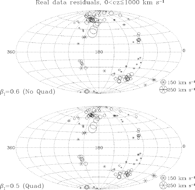
Figure 10: VELMOD velocity residuals plotted on the sky in Galactic coordinates, for objects with $0<cz_{{\rm LG}}\leq 1000\ {\rm km}\,{\rm s}^{-1}.$ The top panel is for the $\beta_{I}=0.6$ run without the quadrupole. The bottom panel is for the $\beta_{I}=0.5$ run with the quadrupole modeled. Open circles indicate objects that are inflowing relative to the IRAS prediction; stars indicate outflowing objects.

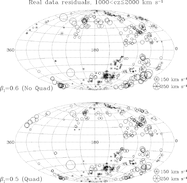
Figure 11: Same as Figure 10, but for objects with $1000<cz_{{\rm LG}}\leq 2000\ {\rm km}\,{\rm s}^{-1}.$

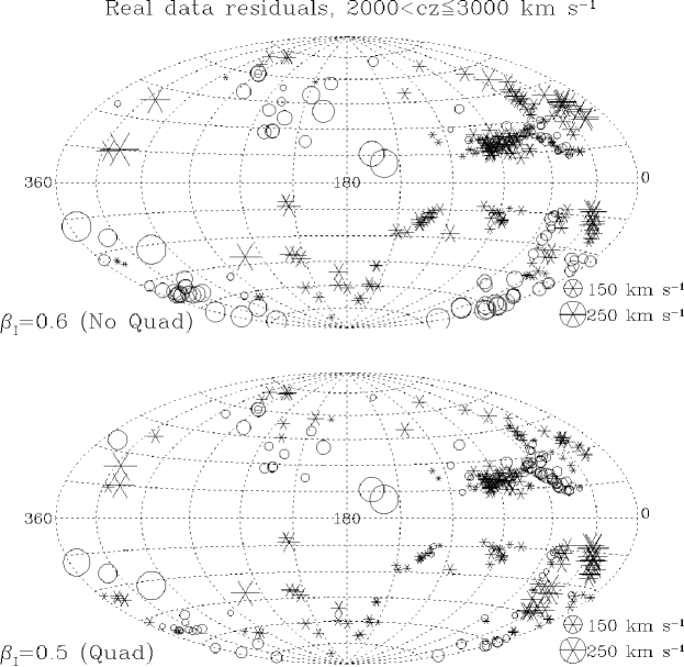
Figure 12: Same as Figure 10, but for objects with $2000<cz_{{\rm LG}}\leq 3000\ {\rm km}\,{\rm s}^{-1}.$

5.1 Sky Maps of VELMOD Residuals

VELMOD does not assign galaxies a unique distance (§ 2.2.1). Thus, there is no unique measure of the amount by which their observed and predicted peculiar velocities differ. However, there is a well-defined expected apparent magnitude for each object,

$$E(m|\eta,cz)=\int_{-\infty}^{\infty}\!m\,P(m|\eta,cz)\,dm\,,$$ (21)

where $P(m|\eta,cz)$ is given by Eq. (11). Similarly, the rms dispersion about this expected value is

$$\Delta m=\sqrt{E(m^{2}|\eta,cz)-\left[E(m|\eta,cz)\right]^{2}}\,.$$ (22)

Note that $\Delta m$ is not equal to the TF scatter; it also includes the combined effects of velocity noise, peculiar velocity gradients, and density changes along the line of sight. At large distances, $\Delta m$ tends toward $\sigma_{{\rm TF}}$ (although dispersion bias can make it smaller; cf. Willick 1994). With the above definitions, one can define a normalized magnitude residual for each galaxy

$$\delta_{m}=\frac{m-E(m|\eta,cz)}{\Delta m}\,.$$ (23)

The normalized residual has the virtue of having unit variance for all objects. In contrast, the variance of the unnormalized magnitude residual $m-E(m|\eta,cz)$ depends on distance (velocity noise is more important for nearby objects), while the variance of a peculiar velocity residual formed from the magnitude residual (Eq. 24 below) grows with distance. The normalized magnitude residual $\delta_{m}$ is a measure of the correctness of the IRAS velocity model. If, in a given region, $\delta_{m}>0$ in the mean, galaxies in that part of space must be more distant than IRAS predicts them to be—i.e., they have negative radial peculiar velocity relative to the IRAS prediction. Regions in which $\delta_{m}<0$ in the mean have positive radial peculiar velocities relative to IRAS.

We will use the normalized magnitude residual below in our quantitative analysis of residuals, but let us first visualize this residual field on the sky, by converting $\delta_{m}$ into the corresponding radial peculiar velocity residual $\delta u.$ Were we to do this for each galaxy individually, the $\sim\,$20% distance errors due to TF scatter would completely hide systematic departures from the IRAS model. Instead, we will compute smoothed velocity residuals. This procedure is most well-behaved if we first smooth $\delta_{m}$ and then convert the result into $\delta u.$ We first place each galaxy at the distance $d$ assigned it by the IRAS velocity model; this is a redshift space distance so our calculation is unaffected by Malmquist bias. Then for each galaxy $i$, we compute a smoothed residual $\delta_{m,i}^{s}$ as the weighted sum of the residuals $\delta_{m}$ of itself and its neighbors $j$, where the weights are $w_{ij}=\exp\left(-d_{ij}^{2}/2S_{i}^{2}\right),$ and $d_{ij}$ is the IRAS-predicted distance between galaxies $i$ and $j.$ We take the smoothing length $S_{i}$ to be $S_{i}=d_{i}/5.$ The smoothed residual $\delta_{m,i}^{s}$ is converted into a smoothed velocity residual according to

$$\delta u_{i}^{s}=d_{i}\left[1-f_{i}10^{0.2(\delta_{m,i}^{s}\times\Delta m_{i})}\right]\,,$$ (24)

where $\Delta m_{i}$ is given by Eq. (22). The quantity $f_{i}$ is given by $\exp\left(-\Delta_{i}^{2}/2\right),$ where $\Delta_{i}=0.46\Delta m_{i}/\sqrt{\sum_{j}w_{ij}};$ it guarantees that $\delta u_{i}^{s},$ which is log-normally distributed, has expectation value zero if $\Delta m_{i}$ (which is normally distributed) does (cf. Willick 1991, § 6.3, for details).

In Figures 10, 11, and 12 we plot VELMOD velocity residuals on the sky for the redshift ranges 0–1000 km s^-1, 1000–2000 km s^-1, and 2000–3000 km s^-1 respectively. In each figure, the top panel shows residuals from the $\beta_{I}=0.6$ (no quadrupole) fit, and the bottom panel shows residuals from the $\beta_{I}=0.5$ (quadrupole modeled) fit, the VELMOD runs closest to the maximum likelihood value of $\beta_{I}$ for each case. The plots reveal why the addition of the quadrupole results in a large increase of likelihood. In each redshift range, the no-quadrupole fits show coherent negative velocity residuals in both the Ursa Major region ($l\simeq 150^{\circ}\,,$ $b\simeq 65^{\circ}\,$), and at $b\simeq-60^{\circ}\,,$ $l\lower 2.15277pt\hbox{$\,\buildrel<\over{\sim}\,$}30^{\circ}\,$ and $l\lower 2.15277pt\hbox{$\,\buildrel>\over{\sim}\,$}330^{\circ}\,.$ In both of these regions, the addition of the quadrupole greatly reduces the amplitude of the residuals. In other parts of the sky, smaller but still significant coherent residuals are reduced with the addition of the quadrupole. This shows that the pattern of departure from the pure IRAS velocity field is well-modeled by a quadrupolar flow of modest amplitude, and therefore has the simple physical interpretation we discussed in § 4.4.

In the bottom panels, it is difficult to find any well-sampled region within $2000\ {\rm km}\,{\rm s}^{-1}$ where $|\delta u|\lower 2.15277pt\hbox{$\,\buildrel>\over{\sim}\,$}100\ {\rm km}\,{\rm s}^{-1}.$ This is all the more remarkable because the TF errors themselves are of order 300 km s^-1 per galaxy at a distance of 1500 km s^-1. Figure 12 does show several high-amplitude residuals. However, at 2500 km s^-1, the TF residual for a single object is 500 km s^-1, so when the effective number of galaxies per smoothing length is only a few, velocity residuals of several hundred km s^-1 are expected from TF scatter only. In well-sampled regions, one sees that in general $|\delta u|\lower 2.15277pt\hbox{$\,\buildrel<\over{\sim}\,$}150\ {\rm km}\,{\rm s}^{-1},$ the only exception being a patch of large ($\lower 2.15277pt\hbox{$\,\buildrel>\over{\sim}\,$}250\ {\rm km}\,{\rm s}^{-1}$) positive residuals at $l\simeq 330^{\circ}\,,$ $b\simeq-20^{\circ}.$ In the $b>0^{\circ}\,$ part of the Great Attractor region at $l\simeq 300^{\circ}\,,$ the residuals are $<100\ {\rm km}\,{\rm s}^{-1}$ even in this highest redshift shell. This is significant, given the oft-heard claims that the IRAS model cannot fit the observed flow into the Great Attractor.

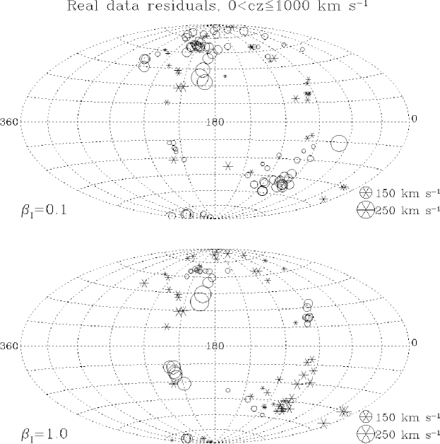
Figure 13: Same as Figure 10, except now results for $\beta_{I}=0.1$ and $\beta_{I}=1.0$ are shown. In each case, the quadrupole is the same as it was for the best fit model ($\beta_{I}=0.5$).

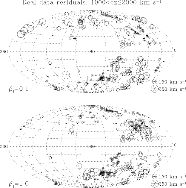
Figure 14: Same as the previous figure, but for objects with $1000<cz_{{\rm LG}}\leq 2000\ {\rm km}\,{\rm s}^{-1}.$

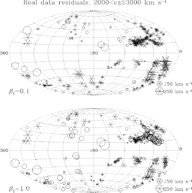
Figure 15: Same as the previous figure, but for objects with $2000<cz_{{\rm LG}}\leq 3000\ {\rm km}\,{\rm s}^{-1}.$

In Figures 13, 14, and 15 we again plot VELMOD residuals on the sky for the three redshift ranges, now for the two values of $\beta_{I}$ most strongly disfavored by the likelihood statistic in the range studied, $\beta_{I}=0.1$ (top panels) and $\beta_{I}=1.0$ (bottom panels). In each plot, the quadrupole of Figure 4 has been included. These plots, which should be compared with the bottom panels of Figures 10, 11, and 12, demonstrate why very low and high $\beta_{I}$ do not fit the TF data well. In each redshift range, these models exhibit large, coherent residuals. For $\beta_{I}=0.1,$ we see large negative peculiar velocities relative to IRAS in the Ursa Major region at $cz\leq 2000\ {\rm km}\,{\rm s}^{-1}.$ Indeed, the residual plot for $\beta_{I}=0.1$ (with quadrupole included) shows many of the same features as the no-quadrupole model with $\beta_{I}=0.6$, because the IRAS field itself contributes some of the needed quadrupole. However, the IRAS contribution scales with $\beta_{I},$ and is thus inadequate at low $\beta_{I}.$ At $\beta_{I}=1.0$ many of the systematic residuals associated with the quadrupole are gone, especially in Ursa Major. However, other regions show highly significant residuals: at $l\simeq 150^{\circ}\,,$ $b\simeq-20^{\circ}\,$ and $cz\leq 1000\ {\rm km}\,{\rm s}^{-1},$ for example, one sees negative peculiar velocity residuals of amplitude $\lower 2.15277pt\hbox{$\,\buildrel>\over{\sim}\,$}200\ {\rm km}\,{\rm s}^{-1},$ which is significant at such small distances. In the same redshift range, at $l=270$–$360^{\circ}\,,$ $b<0^{\circ}\,$ there are positive velocity residuals of amplitude $\lower 2.15277pt\hbox{$\,\buildrel>\over{\sim}\,$}150\ {\rm km}\,{\rm s}^{-1}.$ These regions exhibit much smaller residuals in the $\beta_{I}=0.5$ model.

In the higher redshift shells, the poor fit of the $\beta_{I}=1.0$ model is evidenced chiefly in the direction of the Great Attractor ($l\simeq 300^{\circ}\,,$ $b\simeq 20^{\circ}\,$). For $1000<cz\leq 2000\ {\rm km}\,{\rm s}^{-1},$ this model predicts much too large positive peculiar velocities, so that the data exhibit inflow relative to the model. In the highest redshift bin, the $\beta_{I}=1.0$ model exhibits both positive and negative velocity residuals of high amplitude in the GA direction; residuals of both signs are seen in this region for $\beta_{I}=0.5$ as well, but they are of much smaller amplitude (lower panel of Figure 12). The $\beta_{I}=0.1$ model, on the other hand, predicts too-small positive peculiar velocities in the GA direction at the highest redshifts. Indeed, note that in the $2000<cz_{LG}\leq 3000\ {\rm km}\,{\rm s}^{-1}$ shell, nearly all data points exhibit outflow relative to the $\beta_{I}=0.1$ IRAS predictions, whereas at lower velocities the residuals typically indicate inflow. This global mismatch is more general than the insufficient quadrupole mentioned in the previous paragraph, showing that low $\beta_{I}$ could not yield a good fit even if we were to give VELMOD full freedom in fitting the quadrupole at all $\beta_{I}.$

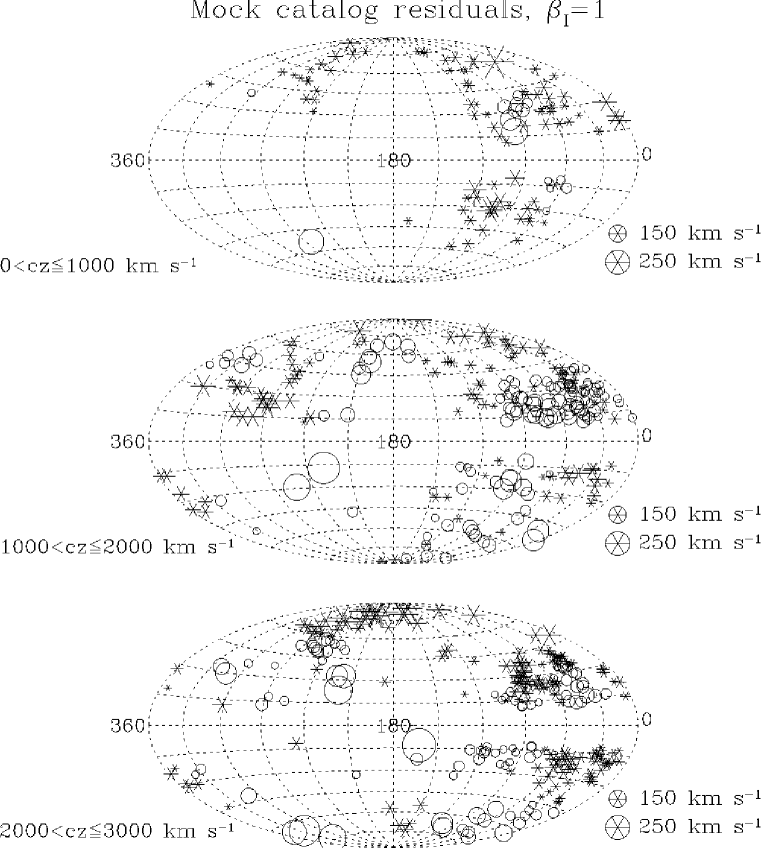
Figure 16: VELMOD velocity residuals for a single mock catalog run using $\beta_{I}=1.0,$ the true value for the mock catalog. (The particular simulation used had a maximum likelihood value of $\beta_{I}=0.963.$) The three panels show residuals for the three redshift ranges used in analyzing the real data.

Although sky plots of residuals argue in favor of the $\beta_{I}=0.5$ plus quadrupole model, the residuals from that model are not manifestly negligible. We will address this issue quantitatively below. For now, however, we can demonstrate qualitatively that the residuals seen in the $\beta_{I}=0.5$ plus quadrupole model are not unexpected by comparing with the mock catalogs, for which the IRAS velocity predictions are known to be a good fit. Figure 16 plots VELMOD velocity residuals with respect to $\beta_{I}=1$ (the correct value) for a single mock catalog. The same three redshift ranges used for the real data are shown. The mock catalog residuals are comparable in amplitude and apparent coherence to the real data. Generally speaking, velocity residuals in well-sampled regions are $\lower 2.15277pt\hbox{$\,\buildrel<\over{\sim}\,$}100\ {\rm km}\,{\rm s}^{-1}$ within 1000 km s^-1, and are $\lower 2.15277pt\hbox{$\,\buildrel<\over{\sim}\,$}200\ {\rm km}\,{\rm s}^{-1}$ at larger distances. One also sees apparent coherence in the mock catalog residual map, as was the case with the real data. The similar amount of apparent coherence in the real and mock data indicates that the former is not a result of a poor fit. The apparent coherence in the residual sky maps is an artifact of the smoothing used to generate them, as we show in the next section.

5.2 Residual Autocorrelation Function

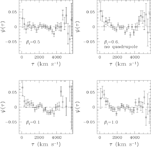
Figure 17: VELMOD residual autocorrelation functions, $\psi(\tau),$ plotted for $\beta_{I}=0.5$ plus quadrupole (best fit model), $\beta_{I}=0.6,$ no quadrupole, $\beta_{I}=0.1$ plus quadrupole, and $\beta_{I}=1.0$ plus quadrupole. In the $\beta_{I}=0.1$ several points at large $\tau$ have residuals that are so large that they fall beyond the plot boundaries.

The sky plots shown above provide visual evidence that the $\beta_{I}=0.5$ plus quadrupole fit has generally small residuals, although they are correlated to some degree. In this section, we quantify these correlations with the residual autocorrelation function

$$\psi(\tau)\equiv\frac{1}{N_{p}(\tau)}\sum\Sb i<j\\ d_{ij}=\tau\pm\Delta\tau\delta_{m,i}\delta_{m,j}\,,$$ (25)

where $\delta_{m}$ was defined in Eq. (23), and the sum is over the $N_{p}(\tau)$ distinct pairs with IRAS predicted separation $d_{ij}$ within $\Delta\tau=100\ {\rm km}\,{\rm s}^{-1}$ of a given value $\tau$. This definition makes $\psi(\tau)$ insensitive to the values of $\sigma_{{\rm TF}}$ and $\sigma_{v}$ (because the $\delta_{m,i}$ are themselves normalized using their maximum likelihood values for each $\beta_{I}$), but sensitive to the residual correlations that signal a poor fit.

In Figure 17, we plot $\psi(\tau)$ versus $\tau$ for the IRAS plus quadrupole models, with $\beta_{I}=0.5,$ $0.1,$ and $1.0,$ as well as the $\beta_{I}=0.6,$ no quadrupole model. The error bars are described below. The model that fits best according to the likelihood statistic, $\beta_{I}=0.5$ plus quadrupole, shows no significant residual correlations on any scale. The correlation function is everywhere consistent with zero, as we would expect if the IRAS velocity field plus the quadrupole is indeed a good fit to the data. Indeed, the absence of residual correlations is the basis for a statement made in § 2.2.1, namely, that the individual galaxy probabilities $P(m|\eta,cz)$ are independent, and thus validates the VELMOD likelihood statistic ${\cal L}_{{\rm forw}}.$

The other models shown in Figure 17 all exhibit significant residual correlations. The $\beta_{I}=0.6,$ no quadrupole model has noticeable correlations on small and large scales, as does the $\beta_{I}=0.1$ plus quadrupole model. Indeed, several of the values of $\psi(\tau)$ for $\beta_{I}=0.1$ are so large that they are off-scale on the plot. The $\beta_{I}=1.0$ plus quadrupole model exhibits strong correlations for $\tau\lower 2.15277pt\hbox{$\,\buildrel<\over{\sim}\,$}2000\ {\rm km}\,{\rm s}^{-1}$, although it is well-behaved on large scales.

5.2.1 Using Residual Correlations to Identify Poor Fits Quantitatively

In order to compare the observed residual correlations with the results from the mock catalogs, we would like to define a single statistic that summarizes the deviation of $\psi(\tau)$ from unity. Let us define $\xi(\tau)\equiv N_{p}(\tau)\psi(\tau)$ (cf. Eq. 25). In Appendix C, we discuss the properties of this statistic in greater detail. As we show there, $\xi(\tau)$ approximates a Gaussian random variable of mean zero and variance $N_{p}(\tau),$ if indeed the VELMOD residuals are uncorrelated on scale $\tau.$ (This property was used to compute the error bars on $\psi(\tau)$ above.) To the degree this approximation is a good one, the quantity

$$\chi^{2}_{\xi}\equiv\sum_{k=1}^{M}\frac{\xi^{2}(\tau_{k})}{N_{p}(\tau_{k})}$$ (26)

will be distributed approximately as a $\chi^{2}$ variable with $M$ degrees of freedom, where $M$ is the number of separate bins in which $\xi(\tau)$ is calculated. In contrast, if the residuals are strongly correlated on any scale $\tau,$ $\chi^{2}_{\xi}$ will significantly exceed its expected value.

However, because a single galaxy will appear in many different pairs in the correlation statistic, both within and between bins in $\tau$, the assumptions made above do not hold rigorously. In Appendix C we explore this issue further. For now, we appeal to the mock catalogs to assess how closely the quantity $\chi^{2}_{\xi}$ follows $\chi^{2}$ statistics. We computed it for each of the 20 mock catalog runs (§ 3) with $\beta_{I}=1.$ We carried out the calculation to a maximum separation of 6400 km s^-1, in bins of width $200\ {\rm km}\,{\rm s}^{-1},$ so that $M=32,$ and found a mean value $\langle\chi^{2}_{\xi}\rangle=27.83\pm 1.82,$ which may be compared with an expected value of $32$ for a true $\chi^{2}$ statistic. The rms scatter in $\chi^{2}_{\xi}$ was $8.15,$ which is the same as that expected for a true $\chi^{2}.$ The difference between the mean and expected values is $2.3\,\sigma$, indicating that $\chi^{2}_{\xi}$ is not exactly a $\chi^{2}$ statistic, for reasons discussed in Appendix C. However, because the departure from true $\chi^{2}$ statstics is small, $\chi^{2}_{\xi}$ is a useful statistic for measuring goodness of fit when calibrated against the mock catalogs.

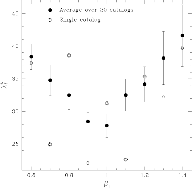
Figure 18: The residual correlation statistic $\chi^{2}_{\xi},$ defined by Eq. 26, plotted as a function of $\beta_{I}$ for the mock catalogs. The solid symbols show an average over 20 mock catalogs; the open symbols show the values obtained for a single mock catalog.

Before presenting $\chi^{2}_{\xi}$ for the real data, we consider its variation with $\beta_{I}$ for the mock catalogs. In Figure 18 we plot the average value of $\chi^{2}_{\xi}$ over the 20 mock catalogs at each value of $\beta_{I}$ for which VELMOD was run. Although the minimum is at $\beta_{I}=1$, it is not nearly as sharp as is that of the likelihood as function of $\beta_{I}$ (e.g., Fig. 2); this statistic does not have the power that the likelihood does for measuring $\beta_{I}$. Indeed, for a single realization (the open symbols), the statistic has several local minima. However, it is apparent that a $\chi^{2}_{\xi}$ value much greater than its expected true value of $\sim\,$28 will indicate a poor fit of the model to the data.

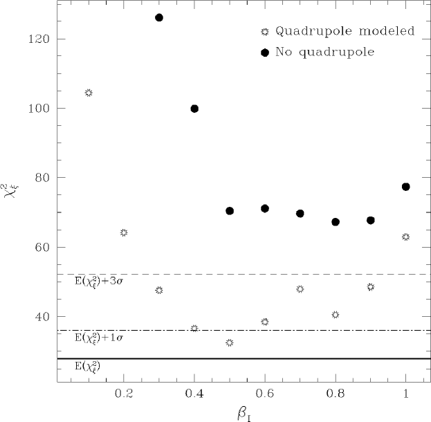
Figure 19: The residual autocorrelation statistic $\chi^{2}_{\xi},$ defined by Eq. 26, plotted as a function of $\beta_{I}$ for the real data, with and without the quadrupole modeled. The heavy solid line shows the expected value of the statistic, which was determined by averaging the derived value for 20 mock catalogs. The two dashed lines show 1- and 3-$\sigma$ deviations from this value. Note that when the quadrupole is not modeled, highly significant residual correlations are detected for all values of $\beta_{I}.$ (The no-quadrupole points for $\beta_{I}=0.1$ and $0.2$ are not shown because their $\chi^{2}_{\xi}$ values are too large.)

In Figure 19, we plot the statistic $\chi^{2}_{\xi}$ as a function of $\beta_{I}$ for the real data, with and without the quadrupole included. The horizontal lines indicate the expected value of $\chi_{\xi}^{2}$, and the $1\,\sigma$ and $3\,\sigma$ deviations from it. Note first that the no-quadrupole model does not provide an acceptable fit for any value of $\beta_{I}.$ This is not a conclusion we could have reached on the basis of the likelihood analysis alone. When the quadrupole is included, the only values of $\beta_{I}$ that are unambiguously ruled out are $\beta_{I}=0.1,$ $0.2,$ and $1.0.$ The best fit model according to VELMOD, $\beta_{I}=0.5$ plus quadrupole, also has the smallest value of $\chi^{2}_{\xi}.$ Given the multiple minima seen for one mock realization in Figure 18, this is not necessarily deeply significant. The statistic $\chi^{2}_{\xi}$ is suitable for identifying models that do not fit the data, but does not have the power of the likelihood statistic for discriminating among those models that do fit.

In summary: the VELMOD likelihood maximization procedure is the proper one for determining which value of $\beta_{I}$ is better than others, but it cannot identify poor fits to our model. The residual correlation statistic $\chi^{2}_{\xi}$ can identify unacceptable fits, but does not have the power to determine which of the acceptable fits is best. We have found that the IRAS velocity field with $\beta_{I}=0.5,$ plus the external quadrupole, is both the best fit of those considered, and is also an acceptable fit. Values of $\beta_{I}>0.9$ and $\beta_{I}<0.3$ are strongly ruled out.

6 Discussion

6.1 What is the value of $\beta_{I}$?

VELMOD recovers the correct answer, $\beta_{I}=1,$ to $<10\%$ accuracy when applied to the mock catalogs. At $\beta_{I}=1,$ the velocity field in the mock Virgo region is significantly triple-valued. Thus VELMOD, despite being close in spirit to Method II, properly treats triple-valuedness. If the strong triple-valuedness one sees at $\beta_{I}=1$ were present in the real universe, VELMOD would not assign it unduly small likelihood. Nonetheless, when VELMOD is applied to the real universe, it returns a value of $\beta_{I}=0.492\pm 0.068$ (quadrupole modeled). This value is quite insensitive to two other quantities treated as free parameters in the velocity field model, the Local Group random velocity ${\bf w}_{{\rm LG}}$ and the small-scale velocity dispersion $\sigma_{v}$ (§ 4.5). Tests with the mock catalogs demonstrated that we obtain an unbiased $\beta_{I}$ using a 300 km s^-1-smoothed IRAS reconstruction (§ 3.1). However, we found that changing to a 500 km s^-1-smoothed reconstruction makes relatively little difference in $\beta_{I}$ (§ 4.6). Finally, neglecting the quadrupole causes $\beta_{I}$ to change by only $\sim\,$$1\,\sigma$. Our conclusion that $\beta_{I}\simeq 0.5\pm 0.07$ is thus robust against systematic effects internal to our method.

The VELMOD result is consistent with the relatively low estimates of $\beta_{I}$ obtained from the Method II analyses of Hudson (1994), Roth (1994), Shaya et al. (1995), DNW, and Schlegel (1996), as well as those derived from comparisons of the IRAS density field with the motion of the Local Group (Strauss et al. 1992b) and from some analyses of the redshift-space anisotropy of the IRAS density field (e.g., Hamilton 1993, 1996; Fisher et al. 1994; Cole, Fisher, & Weinberg 1995; Fisher & Nusser 1996). However, it is apparently inconsistent with estimates of $\beta_{I}$ near unity, as have been found by the POTIRAS analysis (Sigad et al. 1997), measurements of the POTENT fluctuation amplitude (Kolatt & Dekel 1997, Zaroubi et al. 1997), and redshift-space distortions of spherical harmonic expansions of the density field (Fisher, Scharf, & Lahav 1994c; Fisher 1994; Heavens & Taylor 1995).

6.1.1 Why do VELMOD and POTIRAS yield different values of $\beta_{I}$?

We do not yet have a satisfactory explanation of why VELMOD and standard Method II analyses characteristically yield smaller values of $\beta_{I}$ than the Method I POTIRAS approach. One possibility is that the differences stem from the Method I/Method II distinction. However, VELMOD corrects the principal drawback of Method II, the inability to deal with multivalued or flat zones in the redshift-distance relation. Thus, if the Method I/Method II distinction is at the root of the discrepancy, the reason must be more subtle than the drawbacks of standard Method II. Sigad et al. (1997) test for biases in POTIRAS using the same mock catalogs as this paper; they too find their determination of $\beta_{I}$ to be essentially unbiased. The problem could lie with the Malmquist bias corrections that are so crucial to Method I (cf. the discussion in Willick et al. 1997). If these corrections are underestimated for any reason—e.g., the TF scatter is larger than estimated, or the density fluctuations are larger than modeled—a Method I approach will produce too-strong velocity gradients and thus overestimate $\beta_{I}.$ However, the TF scatters used by Sigad et al. (1997) are consistent with those obtained in this paper, and the large POTENT smoothing limits the effect of Malmquist bias in any case. It is thus unlikely that improper Malmquist bias corrections strongly affect the value of $\beta_{I}$ obtained from POTIRAS.

An important difference between VELMOD and POTENT is the Gaussian smoothing scales employed, 300 and 1200 km s^-1 respectively. These very different smoothings could result in different values of $\beta_{I}$ if the effective bias parameters on these scales are different. In order to reconcile VELMOD and POTIRAS, we would need the effective bias parameter to decrease by a factor of $1.7$ between scales of 300 and 1200 km s^-1. Such a scale-dependent biasing has been suggested by the galaxy formation models of Kauffman et al. (1996), but Weinberg (1995) and Jenkins et al. (1996) do not find these trends. A recent analysis by Nusser & Dekel (1997) using a spherical harmonic expansion of the velocity field finds $\beta_{I}=1.0$ for 1200 km s^-1 smoothing, but only 0.6 for 600 km s^-1 smoothing, approaching the value we have found in this paper. Such a change of $\beta_{I}$ with smoothing scale could signal scale-dependent biasing.

Still another difference is the volume considered. We have restricted this analysis to $cz\leq 3000\ {\rm km}\,{\rm s}^{-1}$ (§ 4), whereas the analysis of Sigad et al. (1997) extends to 6000 km s^-1; only $\sim 1/3$ of the points used fall within 3000 km s^-1. If, for whatever reason, $b_{I}$ differed locally from its global value, the VELMOD result could be biased low. In a future paper we will extend the VELMOD analysis to larger distances; however, our preliminary results do not show an increase in $\beta_{I}$ when we do so. In addition to probing a larger volume, the Sigad et al. analysis uses the full Mark III sample, ellipticals included; the possibility of systematic differences between the TF subset we have used in this paper, and the full sample, is difficult to rule out. Finally, it is conceivable that the requirement of pre-calibrating TF relations (POTENT), as opposed to calibrating them simultaneously with fitting the velocity field (VELMOD and Method II generally) accounts for part of the discrepancy. However, fixing the VELMOD TF parameters at their Mark III values has essentially no effect on the derived value of $\beta_{I}$ (§ 4.7). This strongly argues against the notion that a major difference between VELMOD and POTIRAS is the TF relations themselves.

6.1.2 The effect of cosmic scatter

The sphere out to 3000 km s^-1 is small; the rms value of density fluctuations within spheres of this radius is 20% for COBE-normalized CDM. However, this does not propagate to a cosmic scatter error on our derived $\beta_{I}$, for two reasons. First, the IRAS velocity field is determined within a sphere of radius 12,800 km s^-1, within which the rms fluctuations are only a few percent. Thus the peculiar velocity field is subject to very little cosmic scatter. Second, this scatter primarily manifests itself as a monopole term (cf. the discussion in § 4.4), and therefore is fully absorbed into the zero-points of the TF relations (§ 3.3), having no effect on the derived value of $\beta_{I}$.

6.2 Do the IRAS and TF Velocity Fields Agree?

An important conclusion of this paper is that the agreement between the predicted and observed peculiar velocity fields is satisfactory (§ 5), as it must be if the resulting estimate of $\beta_{I}$ is to be believed. This agreement is consistent with the hypothesis that gravitational instability theory correctly describes the relationship between the peculiar velocity and mass density fields. It also suggests that the linear biasing model, Eq. (2), is a reasonable description of the relative distribution of IRAS galaxies and all gravitating matter Gaussian smoothed at $300\ {\rm km}\,{\rm s}^{-1}.$

6.2.1 Comparison with Davis, Nusser, & Willick (1996)

DNW reached a different conclusion. Comparing the IRAS and TF velocity fields with a Method II approach, (ITF; cf. § 2.1) DNW found that the fields do not agree at a statistically acceptable level. In particular, a $\chi^{2}$ statistic resulting from a mode-by-mode comparison of the IRAS and ITF velocity fields was found to be 100 for 55 degrees of freedom. DNW argued that the excessive value of their $\chi^{2}$ statistic resulted primarily from a dipole in the TF velocity field that grows with scale, a feature not seen in the IRAS predictions. They cautioned that, as a result, their maximum likelihood value of $\beta_{I}\sim 0.5$ was not necessarily meaningful.

Why do we find agreement between the TF and IRAS data, while the ITF analysis of DNW did not? We cannot answer this question with assurance, but we can suggest two likely causes of the discrepancy. First, the ITF analysis requires that the raw magnitude and velocity width data of the different samples be placed on a single, uniform system. This was achieved by applying linear transformations to the magnitudes and widths of each sample (Willick et al. 1997). Such a procedure in effect links together the TF zero points of samples that probe different volumes. Any systematic error in matching the data sets will manifest itself in spurious large-scale motions; in particular, the scale-dependent, dipolar flow found by DNW (see, for example, their Figures 12 and 13) is fully degenerate with a zero-point error in the relative TF calibrations of Southern and Northern sky samples. Second, DNW extended their ITF analysis to 6000 km s^-1, whereas we have restricted our analysis to $cz_{{\rm LG}}\leq 3000\ {\rm km}\,{\rm s}^{-1}.$ In so doing, they (like POTIRAS) incorporated several Mark III TF samples (W91CL, HMCL, W91PP, CF) not included in the VELMOD analysis. It is possible that IRAS and Mark III agree locally, but progressively disagree at larger distances. Alternatively, the possible zero point errors mentioned above could affect mainly those Mark III samples used by DNW but not included here, given the agreement we found between the MAT and A82 distances with the VELMOD calibrations (§ 4.7).

Since we believe that the DNW discrepancy between the IRAS and TF velocity fields may well be a result of systematic errors incurred in matching data sets, an effect to which VELMOD is insensitive, we are inclined to give more weight to our present conclusion that the IRAS–TF agreement is satisfactory. However, if in fact the matching of data sets by DNW is validated by ongoing observations aimed at providing reliable North-South homogenization (cf. Strauss 1996b), it will be difficult to escape their conclusion that the predicted and observed velocity fields do not agree on large scales. In that case, it will be necessary to reexamine the conclusions of this paper with regard to the value of $\beta_{I}.$

6.2.2 The Role of the Quadrupole

Our conclusion that the predicted and observed velocity fields agree also depends on the validity of our adopted external quadrupole. Figure 19 shows that only with the quadrupole does our goodness of fit statistic $\chi^{2}_{\xi}$ take on acceptable values. We argue in Appendix B that the 3.3% residual quadrupole we see is mostly due to the systematic difference between the true and Wiener-filtered IRAS density field on large scales. The residual quadrupole in the mock catalogs is appreciably smaller, ${}<1\%$, but this can be understood in terms of the different amount of power on intermediate scales ($2\,\pi/k\approx 100\ h^{-1}$ Mpc) in the mock catalog and the real universe. Thus, the presence of the quadrupole residual is not evidence for a breakdown of our assumptions of gravitational instability theory and linear biasing.

6.3 What is the value of $\Omega?$

Measuring $\beta=\Omega^{0.6}/b$ is an important objective of velocity analysis. Of course, the more important objective is determination of $\Omega$ itself. There are, broadly speaking, two ways to proceed.

6.3.1 Nonlinear Analysis

One may attempt to break the degeneracy between $\Omega$ and biasing by extending gravitational instability theory to the nonlinear dynamical regime. In an earlier phase of the VELMOD project, we attempted to do this; very preliminary results of this effort were described in SW, § 8.1.2. In brief, the IRAS reconstruction was done as described in Appendix A, but a nonlinear generalization of Eq. (1),

$${\bf v}({\bf r})=\frac{f(\Omega)}{4\,\pi}\int d^{3}{\bf r}^{\prime}\,\frac{(1+a^{2}\nu)\delta[\delta_{g}({\bf r}^{\prime});b]+a\nu}{1+a\delta[\delta_{g}({\bf r}^{\prime});b]}\frac{({\bf r}^{\prime}-{\bf r})}{\left|{\bf r}^{\prime}-{\bf r}\right|^{3}}\,,$$ (27)

was used to derive peculiar velocities from the redshift survey density field $\delta_{g}.$ In Eq. (27), $a=0.28$ and $\nu\equiv{\left\langle\delta^{2}\right\rangle}$ is the mean square value of $\delta$ (Ganon et al. 1995; cf., Nusser et al. 1991). Note that the mass fluctuation $\delta$ is written as a generic function of $\delta_{g}$ and $b,$ rather than simply as $\delta_{g}/b.$ This is because once we generalize to nonlinear dynamics, we must allow for the possibility of nonlinear biasing as well. There are many ways one might imagine doing this (SW, § 2.5; Fry & Gaztañaga 1993). Generically, however, all these complications can be expanded to second order to yield a correction to Eq. (3):

$${\bf v}({\bf r})=\frac{\beta}{4\,\pi}\int d^{3}{\bf r}^{\prime}\,\frac{[\delta_{g}({\bf r}^{\prime})+\gamma(\delta_{g}^{2}({\bf r})-\nu)]({\bf r}^{\prime}-{\bf r})}{\left|{\bf r}^{\prime}-{\bf r}\right|^{3}}\,.$$ (28)

where $\gamma$ parameterizes the combined effects of nonlinear dynamics and nonlinear biasing.

We carried out a suite of VELMOD runs using predicted peculiar velocities based on Eq. (28) for a range of values of $\gamma$, both positive and negative. Our hope was that the VELMOD likelihood statistic would be significantly lower for some value of $\gamma$ than for the pure linear case. However, to our surprise, we found that the linear dynamics/linear biasing reconstruction ($\gamma=0$) gives the best likelihood of all. We are not certain as to why this is. Nonlinear dynamics must enter to some degree, because we know for a fact that $\delta_{g}$ is not everywhere $\ll 1,$ and indeed can be quite large with our small smoothing. (We of course do not know whether nonlinear biasing is important.) Nevertheless, the small scatter between the true and IRAS predicted peculiar velocity fields for the mock catalogs (§ 3.2) confirms that the linear IRAS velocity field, smoothed on a 300 km s^-1 scale, is a good match to actual peculiar velocities that arise from gravitational instability, at least in an $N$-body simulation.

A possible explanation of this seeming contradiction is as follows. Our method for predicting peculiar velocities (Appendix A) entails assigning a smooth, continuous density field from discrete redshift survey data—a procedure which takes into account the probability distribution of distance given redshift (Eq. 31), smooths the data with a 300 km s^-1 Gaussian, and applies a Wiener filter—and thus reduces small-scale density enhancements. In doing so, this procedure mimics qualitatively the effects of nonlinear corrections to the velocity-density relation. The good match between the IRAS predictions and the actual peculiar velocities suggests that this mimicry is in fact fortuitously good, to the degree that formal nonlinear corrections are unnecessary.

6.3.2 Constraining $\Omega$ from Independent Estimates of $b_{I}$

The second way to estimate $\Omega,$ given our measurement of $\beta_{I},$ is to constrain $b_{I}$ using independent information. If biasing is independent of scale (cf. the discussion in § 6.1.1), then $b_{I}$ is the ratio of the rms fluctuations of IRAS galaxies on an 8$h^{-1}$ Mpc scale, $\sigma_{8}({\sl IRAS\/}),$ to the corresponding mass density fluctuations, $\sigma_{8}.$ Fisher et al. (1994a) found that $\sigma_{8}({\sl IRAS\/})=0.69\pm 0.04$ in real space. It follows that $\beta_{I}$ can be viewed as a prediction of $\sigma_{8}$ for a given value of $\Omega:$

$$\sigma_{8}=\frac{(0.69\pm 0.04)\,\beta_{I}}{\Omega^{0.6}}\,.$$ (29)

An entirely independent (though highly model-dependent) way to predict $\sigma_{8}$ as a function of $\Omega$ is to use COBE-normalized power spectra for a range of cosmological parameters. Liddle et al. (1995, 1996) have presented fitting functions that provide the normalization of CDM power spectra, in open and flat cosmologies, as a function of $\Omega,$ $\Omega_{\Lambda},$ the Hubble parameter $h\equiv H_{0}/(100\ {\rm km}\,{\rm s}^{-1}\ {{\rm Mpc}}^{-1}),$ and the primordial power spectrum index $n,$ based on the four-year COBE observations (Bennett et al. 1996; Górski et al. 1996). Eke, Cole, & Frenk (1996) used these fitting functions to obtain $\sigma_{8}$ by direct integration of the Liddle et al. power spectra, and have kindly provided us with their code for doing this calculation. We may thus constrain $\sigma_{8}$ by comparing the VELMOD and COBE/CDM predictions of its value, and requiring that they agree to within the errors. This will be the case only for a limited range of $\Omega$ (the “concordance range”). We emphasize, however, that the discusion to follow depends on two uncertain assumptions: first, that the CMB fluctuations measured by COBE can be reliably extrapolated down to 8$h^{-1}$ Mpc scales; and second, that the bias parameter is scale-independent from 3$h^{-1}$ to 8$h^{-1}$ Mpc.

cobe_open_scinv.pscobe_flat_scinv.ps

Figure 20: Predictions of $\sigma_{8}$ as a function of $\Omega$ for open (left panel) and flat (right panel) universes. The lines sloping up and to the right show the COBE-normalized CDM values of $\sigma_{8}$ as a function of $\Omega,$ for four values of the Hubble constant, 55, 65, 75, and 85 km s^-1 Mpc${}^{-1},$ under the assumption of a scale-invariant primordial power spectrum. The line sloping down and to the right shows the result from this paper, $\sigma_{8}=0.69\beta_{I}/\Omega^{0.6}.$ The shaded region represents the 1-$\sigma$ uncertainty in our value of $\beta_{I}.$

In Figure 20, we compare the two constraints on $\sigma_{8}$ for a scale-invariant ($n=1$) power spectrum. The left hand panel shows results for an open (i.e., $\Lambda=0$) universe, and the right hand panel for a spatially flat ($\Omega+\Omega_{\Lambda}=1$) universe. The COBE/CDM predictions (solid lines labeled with the values of the Hubble constant) and the constraint from Eq. (29) (shaded region) scale very differently with $\Omega$, so that the two together give strong constraints on $\sigma_{8}$ and thus $\Omega.$ The shaded region represents the combined VELMOD error on $\beta_{I}$ and the error in $\sigma_{8}({\sl IRAS\/})$ from Fisher et al. (1994a). We do not show corresponding error regions for the COBE/CDM predictions which result from uncertainty in the COBE normalization, because the error in the predicted $\sigma_{8}$ is in fact dominated by the allowed range of $H_{0},$ which we take to be $55\leq H_{0}\leq 85\ {\rm km}\,{\rm s}^{-1}\ {{\rm Mpc}}^{-1}$ based on a number of recent measurements (Sandage et al. 1996; Freedman 1996; Riess, Press, & Kirshner 1996; Mould et al. 1996; Tonry et al. 1997; Kundić et al. 1996).

Figure 20 gives the following constraints for $n=1$. For an open model, the concordance range is $\Omega=0.28$–$0.46$ with the low (high) value corresponding to the highest (lowest) value of $H_{0}$ considered. For the flat model, it is $\Omega=0.16$–$0.34.$ Expressed in terms of the IRAS bias parameter, these ranges correspond to $b_{I}=0.92$–$1.38$ (open) and $b_{I}=0.68$–$1.11$ (flat). We also considered $n\neq 1$ flat models. For example, with $n=0.9$ the concordance ranges are $\Omega=0.19$–$0.40,$ and $0.21$–$0.45,$ depending respectively on whether tensor fluctuations are not, or are, included in the COBE normalization (Liddle et al. 1996b). The corresponding bias parameters are $b_{I}=0.74$–$1.21$ and $b_{I}=0.80$–$1.29.$

Two salient points follow from this comparison. First, if $H_{0}\geq 60\ {\rm km}\,{\rm s}^{-1}\ {{\rm Mpc}}^{-1},$ the concordance range for the flat, $n=1$ models requires $\Omega\lower 2.15277pt\hbox{$\,\buildrel<\over{\sim}\,$}0.30,$ implying $\Omega_{\Lambda}\lower 2.15277pt\hbox{$\,\buildrel>\over{\sim}\,$}0.70.$ However, studies of gravitational lensing have placed an upper limit of $\Omega_{\Lambda}\leq 0.65$ at 95% confidence (Maoz & Rix 1993; Kochanek 1996), while a recent analysis of intermediate-redshift Type Ia Supernovae (Perlmutter et al. 1996) indicates $\Omega_{\Lambda}\leq 0.50$ at 95% confidence (both of these constraints apply when a flat universe is assumed). This contradiction consitutes evidence against a flat universe with a scale-invariant primordial power spectrum index and $H_{0}\geq 60\ {\rm km}\,{\rm s}^{-1}\ {{\rm Mpc}}^{-1}.$ If $n<1.0,$ one can more easily accommodate flat universes with $\Omega_{\Lambda}<0.65,$ provided the Hubble constant is $\lower 2.15277pt\hbox{$\,\buildrel<\over{\sim}\,$}70\ {\rm km}\,{\rm s}^{-1}\ {{\rm Mpc}}^{-1}.$ The second point is that the combined VELMOD and COBE/CDM predictions of $\sigma_{8}$ are extremely difficult to reconcile with an Einstein-de Sitter universe for most reasonable values of the remaining cosmological parameters. If one assumes $n\geq 0.9,$ a Hubble constant $\lower 2.15277pt\hbox{$\,\buildrel<\over{\sim}\,$}30\ {\rm km}\,{\rm s}^{-1}\ {{\rm Mpc}}^{-1},$ far below current observational limits, would be required for the concordance range to include $\Omega=1.$ Alternatively, if $H_{0}=50\ {\rm km}\,{\rm s}^{-1}\ {{\rm Mpc}}^{-1},$ one would require a primordial power spectrum index $n=0.7$ and tensor fluctuation contributions to the CMB anisotropies. Such a power-spectrum index is at the lowest end of the range currently considered plausible in inflationary universe scenarios (e.g., Steinhardt 1996).

6.4 Summary

We have described a new maximum likelihood method, VELMOD, for comparing Tully-Fisher data with predicted peculiar velocity fields from redshift surveys. We implemented the method for a $cz_{{\rm LG}}\leq 3000\ {\rm km}\,{\rm s}^{-1}$ TF subsample from the Mark III catalog (Willick et al. 1997), and velocity fields predicted from the 1.2 Jy IRAS redshift survey (Fisher et al. 1995). The velocity field prediction is dependent on the value of $\beta_{I}\equiv\Omega^{0.6}/b_{I},$ where $b_{I}$ is the bias parameter for IRAS galaxies at 300 km s^-1 Gaussian smoothing. We maximized likelihood with respect to $\beta_{I},$ the parameters of the TF relation, and several other velocity parameters.

We applied our method to 20 mock Mark III and IRAS catalogs constructed to mimic the properties of the real data. The mock catalogs were drawn from an $\Omega=1$ $N$-body simulation and were constructed to ensure $b_{I}=1.$ Thus, the mock catalogs satisfy $\beta_{I}=1.$ Our VELMOD runs with the twenty mock catalogs returned a mean value of $\beta_{I}=0.984\pm 0.018,$ consistent with the statement that VELMOD yields an unbiased value of $\beta_{I}.$ In addition, our mock catalog tests enabled us to assign reliable 1-$\sigma$ errors to our estimates of $\beta_{I},$ and showed that our other derived parameters, including those of the TF relation and the small-scale velocity noise, are also unbiased. Because the mock catalogs came from an $\Omega=1$ universe, triple valued zones in the mock Virgo region were strong, but were properly handled by the VELMOD analysis.

When VELMOD was applied to the real Mark III data, a considerably smaller value of $\beta_{I}$ was derived. If we assume that the IRAS-predicted velocity field fully describes the actual one, we obtain $\beta_{I}=0.563\pm 0.074.$ However, the residuals from this fit were large and coherent; fitting them by a quadrupolar flow gave a maximum likelihood value of $\beta_{I}=0.492\pm 0.068$. The quadrupole points toward the Ursa Major cluster, and has an rms amplitude of 3.3% of the Hubble flow. In Appendix B, we show analytically that a quadrupole of this amplitude is expected given the way that we smooth the density field; its presence is not a sign that the IRAS galaxies do not trace the mass responsible for the local flow field. An analysis of the fit residuals demonstrated that the IRAS-predicted peculiar velocity field, with the external quadrupole, provides a statistically acceptable fit to the TF data within 3000 km s^-1. The data are thus consistent with the hypothesis that the peculiar velocities are due to the gravitational effects of a mass distribution that is proportional to the IRAS galaxy distribution. We also find that the data are consistent with a very quiet flow field; the one-dimensional rms noise in the velocity field relative to the IRAS model is $125\pm 20\ {\rm km}\,{\rm s}^{-1}.$

The value of $\beta_{I}$ obtained here may also be thought of as a measurement of the rms mass density fluctuations $\sigma_{8}$ as a function of $\Omega.$ Similarly, COBE-normalized CDM power spectra predict a value of $\sigma_{8}$ as a function of $\Omega$ and other cosmological parameters. If we require that the VELMOD and COBE-normalized calculations agree, we can constrain the value of $\Omega.$ For scale invariant, $\Lambda=0$ universes, we derive the constraints $0.28\lower 2.15277pt\hbox{$\,\buildrel<\over{\sim}\,$}\Omega\lower 2.15277pt\hbox{$\,\buildrel<\over{\sim}\,$}0.46$ for for $85\lower 2.15277pt\hbox{$\,\buildrel>\over{\sim}\,$}H_{0}\lower 2.15277pt\hbox{$\,\buildrel>\over{\sim}\,$}55\ {\rm km}\,{\rm s}^{-1}\ {{\rm Mpc}}^{-1}.$ For scale-invariant, flat universes we find $0.16\lower 2.15277pt\hbox{$\,\buildrel<\over{\sim}\,$}\Omega\lower 2.15277pt\hbox{$\,\buildrel<\over{\sim}\,$}0.34$ for the same range of $H_{0}.$ The constraints on $\Omega$ shift to higher values (§ 6.3.2) if the primordial power spectra are “tilted,” $n<1,$ and if tensor fluctuations are present. However, both extreme tilt ($n\leq 0.7$) and a Hubble constant at the lowest end of the observationally allowed range ($H_{0}\leq 50\ {\rm km}\,{\rm s}^{-1}\ {{\rm Mpc}}^{-1}$) would be required to reconcile these results with an Einstein-de Sitter universe.

The conclusions of the previous paragraph all rest, of course, on the validity of our measurement of $\beta_{I}.$ Tests with mock catalogs show that, subject to our basic assumptions, this measurement is reliable to within the quoted errors. We have identified two ways these assumptions can break down. First, the effective bias factor $b_{I}$ could depend on scale. In that case, our measurement of $\beta_{I},$ which reflects a 300 km s^-1 Gaussian smoothing scale, might not be the same as a measurement obtained at larger smoothing; it would not then be valid to equate the estimate of $\sigma_{8}$ obtained from Eq. 29 with the COBE/CDM prediction. Second, although we have found agreement between the predicted and observed peculiar velocities within 3000 km s^-1, DNW found disagreement on larger scales. If the DNW result is validated by future observations (Strauss 1996b) aimed at improved TF calibration across the sky, our present claim of TF-IRAS agreement will be undermined.

There are several areas for further work. One, alluded to in several places in this paper, is to extend our analysis to larger redshift, using both the forward and inverse forms of the TF relation. This can be done both the Mark III data, and with the extensive new TF (Mathewson et al. 1994; Giovanelli et al. 1997) and $D_{n}$-$\sigma$ (Saglia et al. 1996) samples that are being compiled. We should also consider extending this work to other distance indicators; surface brightness fluctuation galaxies (Tonry et al. 1997), with their accurate sampling of the nearby velocity field, are natural candidates for the VELMOD analysis. On the modeling side, this work has left us with several conundrums, the most puzzling of which is why the linear IRAS model does so well with a smoothing scale of 300 km s^-1. More work is needed with $N$-body simulations to understand this. Finally, we will not have a coherent picture of the relationship between the velocity and density fields until we can understand the different values of $\beta_{I}$ obtained by VELMOD and POTIRAS.

Appendix A The IRAS Velocity-Density Reconstruction

The redshifts of galaxies in the IRAS sample are affected by the same peculiar velocities that one is attempting to measure in the Mark III dataset. If we measure redshifts $cz$ in the rest frame of the Local Group, then:

$$cz=r+\hat{\bf r}\cdot\left[{\bf v}({\bf r})-{\bf v}({\bf 0})\right]\quad,$$ (30)

where v(0) is the peculiar velocity of the Local Group, and ${\bf v}({\bf r})$ is the peculiar velocity at position ${\bf r}.$ Indeed, because the galaxy density field shows coherence, the galaxy density field measured in redshift space $\delta_{g}({\bf s})$ differs systematically from that in real space, $\delta_{g}({\bf r})$, as was first described in detail by Kaiser (1987; cf., SW; Strauss 1996a for reviews). Linear perturbation theory assuming gravitational instability enable us to correct for the effects of these velocities. We use here the iteration technique described by Yahil et al. (1991) and Strauss et al. (1992c), as updated by Sigad et al. (1997). The density and velocity field are calculated within a sphere of radius 12,800 km s^-1; the density fluctuation field is assumed to be zero beyond this radius. Here we very briefly reiterate the improvements described in the Sigad et al. paper, and emphasize certain differences from the approach there.

In regions in which the IRAS velocity field model predicts a non-monotonic relation between redshift and distance along a given line of sight, it becomes ambiguous how to assign a distance to a galaxy given its redshift (Figure 1). Our approach is similar to that used throughout this paper: we use our assumed density and velocity field to calculate a probability distribution of a galaxy along a given line of sight.

Along a given line of sight, we ask for the joint probability distribution of observing a galaxy along a given line of sight, with redshift $cz$, flux density $f$ and (unknown) distance $r$:

$$P(cz,f,r)=P(cz|r)\times P(f|r)\times P(r)\quad;$$ (31)

compare with Eq. (5). The first term is given by our velocity field model along the line of sight, and is thus given by Eq. (9). For the iteration code, we set $\sigma_{v}=150\ {\rm km}\,{\rm s}^{-1}$, independent of position, similar to the best fit value we find when we fit for $\sigma_{v}$ from the velocity field data.

The second term is given by the luminosity function of galaxies:

$$P(f|r)=\Phi(L=4\,\pi r^{2}\nu f){dL\over df}\propto r^{2}\Phi(L)\quad,$$ (32)

where the derivative is needed because the probability density is defined in terms of $f$, not $L.$ Finally, the third term in Eq. (31) is given by the galaxy density distribution along the line of sight, Eq. (8).

As described in Sigad et al. (1997), the calculations of the velocity and density fields are done on a Cartesian grid. Our approach therefore is to assign each galaxy to the grid via cloud-in-cell (weighting by the selection function, of course), where (unlike Sigad et al. 1997) we distribute each galaxy along the line of sight according to the distribution function of expected distance, Eq. 31. In order to calculate the selection function for an object, we of course need to have a definite position for it; for this purpose, we assign it the expectation value of its distance, following Sigad et al. (1997):

$${\left\langle r\right\rangle}={\int rP(cz,f,r)\,dr\over\int P(cz,f,r)\,dr}.$$ (33)

Sigad et al. (1997) discuss the use of various filtering techniques to suppress the shot noise in the derived density and velocity fields. While they argue for the use of a power-preserving filter for the comparison of the IRAS and POTENT density fields, we have found through extensive experimentation with mock catalogs that for the VELMOD analysis, a Wiener filter gives the best comparison between the density field and the peculiar velocity data.

Finally, we found that when the iteration technique was run to values of $\beta\lower 2.15277pt\hbox{$\,\buildrel>\over{\sim}\,$}1$, the density field became unstable in the regions around triple-valued zones, oscillating between iterations. We were able to suppress these by averaging the derived density field at each iteration with that of the iteration preceding it. This has no strong effect on the derived density field for $\beta<1$.

Appendix B The Residual Quadrupole

In this Appendix, we calculate the expected amplitude of the velocity quadrupole generated by density fluctuations both external to the IRAS sample (i.e., outside of $R=12,800\,{\rm km}\,{\rm s}^{-1}$), and internal to it, due to the difference between the true density field and the noisy, smoothed estimation of the density field we have from the IRAS redshift survey. The IRAS excluded zone is another potential source of quadrupole error, but it is filled in by interpolation from regions above and below the excluded zone (Yahil et al. 1991), a procedure which agrees well with a multipole interpolation procedure based on spherical harmonics, at least for the $10^{\circ}$ wide IRAS zone of avoidance (Lahav et al. 1994).

B.1 The Quadrupole Induced by Fluctuations Beyond the IRAS Volume

We express peculiar velocity in terms of a potential function $\Phi({\bf r})$, such that the radial component of the velocity field is given by $u(r)=-\partial\Phi/\partial r.$ We will isolate the quadrupole component of this potential, and calculate its angle-averaged rms contribution.

The contribution to $\Phi$ from material at distances $>R$ is given by

$$\Phi({\bf r})=-\frac{f(\Omega)}{4\pi}\int_{|{\bf r}^{\prime}|>R}d^{3}{\bf r}^{\prime}\,\frac{\delta({\bf r}^{\prime})}{|{\bf r}-{\bf r}^{\prime}|}\,.$$ (34)

Here, $\delta$ is the mass, not the galaxy, density fluctuation. We now expand the denominator in the integrand in terms of spherical harmonics (e.g., Jackson 1976, Eq. 3.70) and isolate the quadrupole term to obtain

$$\Phi_{Q}({\bf r})=-\frac{f(\Omega)r^{2}}{5}\sum_{m=-2}^{2}Y_{2m}(\omega)\int_{R}^{\infty}\!\frac{dr^{\prime}}{r^{\prime}}\int d\omega^{\prime}\,\delta({\bf r}^{\prime})\,Y_{2m}^{*}(\omega^{\prime})\,.$$ (35)

where $\omega$ is solid angle. Taking the radial component of the quadrupole velocity $u_{Q}=-\partial\Phi_{Q}/\partial r$, squaring, and averaging over solid angle gives, after several steps of algebra:

$$u_{Q,rms}^{2}(r)=\frac{1}{4\pi}\int\!d\omega\,u_{Q}^{2}({\bf r})$$

$$=\left(\frac{2f(\Omega)r}{5}\right)^{2}\sum_{mm^{\prime}}C_{2m}C^{*}_{2m^{\prime}}\frac{1}{4\pi}\int d\omega\,Y_{2m}(\omega)Y^{*}_{2m^{\prime}}(\omega)=\left(\frac{2f(\Omega)r}{5}\right)^{2}\frac{1}{4\pi}\sum_{m}|C_{2m}|^{2}\,,$$ (36)

where the last step follows from the orthonormality of the $Y_{lm}$’s, and for convenience we have defined the five complex coefficients

$$C_{2m}[R;\delta]\equiv\int_{R}^{\infty}\!\frac{dr^{\prime}}{r^{\prime}}\int d\omega^{\prime}\,\delta({\bf r}^{\prime})\,Y_{2m}^{*}(\omega^{\prime})\,.$$ (37)

The expectation value of $|C_{2m}|^{2}$ is independent of $m$, so when we take the expectation value of Eq. (36), we can replace the sum with 5 times ${\left\langle C_{20}^{2}\right\rangle}$:

$$\langle u_{Q,rms}^{2}(r)\rangle=\left(\frac{2f(\Omega)\,r}{5}\right)^{2}\!\times\frac{5}{4\pi}\,\langle C_{20}^{2}\rangle\,.$$ (38)

Using the definition of $Y_{20}$ in terms of the second Legendre polynomial $P_{2}$ in Eq. (37) and Eq. (38) gives

$${\left\langle u_{Q,rms}^{2}(r)\right\rangle}=(f(\Omega)\,r)^{2}\int_{R}^{\infty}\frac{dr_{1}}{r_{1}}\int_{R}^{\infty}\frac{dr_{2}}{r_{2}}\int_{-1}^{1}\int_{-1}^{1}d\mu_{1}d\mu_{2}\,P_{2}(\mu_{1})P_{2}(\mu_{2})\,\xi(|{\bf r}_{2}-{\bf r}_{1}|)\,.$$ (39)

Expressing the correlation function $\xi$ as the Fourier Transform of the power spectrum $P(k)$ (e.g., SW, Eq. 46) allows the integrals over ${\bf r}_{1}$ and ${\bf r}_{2}$ to separate. This yields

$$\langle u^{2}_{Q,rms}(r)\rangle=\frac{(f(\Omega)\,r)^{2}}{(2\pi)^{3}}\int d^{3}{\bf k}\,P(k)\,\widetilde{W}^{2}(kR)\,,$$ (40)

where the kernel is given by

$$\widetilde{W}(kR)=\int_{R}^{\infty}{dr\over r}\int_{-1}^{1}\!d\mu\,e^{ikr\mu}P_{2}(\mu)=-2\int_{R}^{\infty}\!dr\,\frac{j_{2}(kr)}{r}={2\,j_{1}(kR)\over kR}\,,$$ (41)

and $j_{n}$ is the $n$-th order spherical Bessel function. Comparison of Eqs. (40) and (41) with Eqs. (37) and (38) of SW allows us to recast our result as

$$r^{-1}{\left\langle u_{Q,rms}^{2}(r)\right\rangle}^{1/2}=\frac{2f(\Omega)}{3}\,\sigma_{R}$$ (42)

for the expected rms quadrupole velocity on a sphere due to mass density fluctuations at distances $>R,$ expressed as a fraction of Hubble flow. Here $\sigma^{2}_{R}$ is the variance in the mass overdensity within spheres of radius $R.$ As mentioned in the text, this gives a fractional quadrupole of the order of 1-2$\,\%$ for a variety of COBE-normalized power spectra.

B.2 The Effects of Wiener Filtering and Shot Noise

The Wiener filter operates on the Fourier Transform of the IRAS density field. The final density field differs from the true density fiels for two reasons: the discreteness of the galaxy distribution gives rise to shot noise, and the Wiener filter, while suppressing shot noise, also suppresses the density field itself. We calculate the contribution to the quadrupole from both effects.

Let $\tilde{\delta}_{T}({\bf k})$ represent the true Fourier component of the underlying (noiseless) density field at wavevector ${\bf k}$; the quantity with which we calculate the velocity field is the Wiener-filtered noisy image, whose Fourier modes are given by:

$$\tilde{\delta}({\bf k})=h(k,r)[\tilde{\delta}_{T}({\bf k})+\epsilon(k)]\,,$$ (43)

where the Wiener filter itself is (e.g., Zaroubi et al. 1995):

$$h(k,r)={P(k)\over P(k)+(n_{1}\phi(r))^{-1}}\,,$$ (44)

and $P(k)$ is set a priori; we used a functional fit to the IRAS power spectrum found by Fisher et al. (1993). The noise term in the denominator of the Wiener filter is independent of $k$ (cf., Fisher et al. 1993; SW, § 5.3); however, it is dependent on the density of galaxies, which is a decreasing function of distance in the flux-limited IRAS sample. As explained in Sigad et al. (1997), we therefore calculate a series of Wiener-filtered density fields for different noise levels, and interpolate between them to find the appropriate density field at any given distance.

We wish to calculate the quadrupole due to the error in the derived density field, i.e., that due to the difference between Eq. (43) and $\tilde{\delta}_{T}({\bf k})$. If we expand the density field in Eq. (37) into its Fourier components, substitute this difference for each component, and square the result, we find the rms contribution to $u_{Q}$ due to the Wiener filter:

$${\left\langle u_{Q,Wiener}^{2}\right\rangle}={(r\,f(\Omega))^{2}\over(2\,\pi)^{8}}\int d^{3}{\bf k}_{1}d^{3}{\bf k}_{2}\int{d^{3}{\bf r}_{1}\over r_{1}^{3}}{d^{3}{\bf r}_{2}\over r_{2}^{3}}P_{2}(\mu_{1})P_{2}(\mu_{2})\exp[i({\bf k}_{1}\cdot{\bf r}_{1}-{\bf k}_{2}\cdot{\bf r}_{2})]\times$$

$${\left\langle\left[(h(k_{1},r_{1})-1)\tilde{\delta}_{T}({\bf k}_{1})+h(k_{1},r_{1})\epsilon(k_{1})\right]\,\left[(h(k_{2},r_{2})-1)\tilde{\delta}_{T}({\bf k}_{2})+h(k_{2},r_{2})\epsilon(k_{2})\right]\right\rangle}\,.$$ (45)

This rather horrific expression can be simplified by multiplying out the term in brackets, realizing that the cross-terms vanish and that ${\left\langle\tilde{\delta}_{T}({\bf k}_{1})\tilde{\delta}_{T}({\bf k}_{2})\right\rangle}=(2\,\pi)^{3}P_{T}(k)\delta_{D}({\bf k}_{1}-{\bf k}_{2})$, where $P_{T}(k)$ is the true underlying power spectrum, not necessarily the same as that assumed in Eq. (44). We then get two terms, one depending on the power spectrum, and the other due to shot noise. For the first term, the integrals over ${\bf r}_{1}$ and ${\bf r}_{2}$ separate to give:

$$\langle u^{2}_{Q,Wiener}(r)\rangle=\frac{(f(\Omega)\,r)^{2}}{(2\pi)^{3}}\int d^{3}{\bf k}\,P_{T}(k)\,\widetilde{W}^{2}_{\Delta}(kR)+{\left\langle u^{2}_{Q,shot}\right\rangle}\,,$$ (46)

where the new window function is given by

$$\widetilde{W}_{\Delta}(k,R_{1},R)=-2\int_{R_{1}}^{R}\!dr\,\frac{j_{2}(kr)}{r}[h(k,r)-1)]\,;$$ (47)

compare with Eq. (41). We integrate from the outer volume of our peculiar velocity sample, $R_{1}=3000{\rm km}\,{\rm s}^{-1},$ to $R=12,800$ km s^-1; at smaller radii, the contribution to the quadrupole goes like $r^{-2}$, not $r$, and this is not included in our modelling of the quadrupole (Eq. 19). The contribution to the quadrupole from this term is between 1.5 and 3%, depending on which model we take for the true power spectrum. This is pleasingly close to the value we find for the real universe. The mock catalogs have a power spectrum set by the observed IRAS power spectrum (of course, with a cutoff at $k<2\,\pi/L$), and thus give a somewhat smaller contribution to this integral, about 1%.

Let us now calculate the shot noise contribution to the quadrupole. It is given by:

$${\left\langle u^{2}_{Q,shot}\right\rangle}={(r\,\beta)^{2}\over(2\,\pi)^{8}}\int d^{3}{\bf k}_{1}d^{3}{\bf k}_{2}\int{d^{3}{\bf r}_{1}\over r_{1}^{3}}{d^{3}{\bf r}_{2}\over r_{2}^{3}}P_{2}(\mu_{1})P_{2}(\mu_{2})\exp[i({\bf k}_{1}\cdot{\bf r}_{1}-{\bf k}_{2}\cdot{\bf r}_{2})]\,{\left\langle h(k_{1},r_{1})\epsilon(k_{1})\,h(k_{2},r_{2})\epsilon(k_{2})\right\rangle}\,.$$ (48)

Notice now the dependence on $\beta$, not $\Omega$; here we will make no reference to a COBE-normalized power spectrum. The Fourier modes are calculated in a box of side $L=25,600\ {\rm km}\,{\rm s}^{-1}$, and therefore are uncorrelated for $\Delta k>2\,\pi/L$. Thus we can write the product of the two shot noise terms as a Dirac delta function:

$${\left\langle\epsilon({\bf k}_{1})\epsilon({\bf k}_{2})\right\rangle}={\left\langle\epsilon^{2}({\bf k}_{1})\right\rangle}\left({2\,\pi\over L}\right)^{3}\delta_{D}({\bf k}_{1}-{\bf k}_{2})=\left({2\,\pi\over L}\right)^{3}\delta_{D}({\bf k}_{1}-{\bf k}_{2})\int d^{3}{\bf r}{1\over n_{1}\phi(r)}\,;$$ (49)

the expression for ${\left\langle\epsilon^{2}({\bf k})\right\rangle}$ comes from Fisher et al. (1993). When we insert Eq. (49) into Eq. (48), the latter simplifies dramatically. The integrals over ${\bf r}_{1}$ and ${\bf r}_{2}$ now separate, giving:

$$\langle u_{Q,shot}^{2}(r)\rangle={(r\beta)^{2}\over(2\,\pi)^{3}}\int{d^{3}{\bf k}\over L^{3}}\left(\int d^{3}{\bf r}^{\prime}{1\over{n_{1}\phi(r^{\prime})}}\right)\,W^{2}_{shot}(k)\,,$$ (50)

where the shot noise window function looks very similar to what we have seen before:

$$W_{shot}(k,R_{1},R)=-2\int_{R_{1}}^{R}\!dr\,\frac{j_{2}(kr)}{r}h(k,r)\,.$$ (51)

Notice that unlike the previous calculation, this result is independent of the true power spectrum. If we calculate this using the observed IRAS selection function, integrating from 3000 km s^-1 to 12,800 km s^-1, we find an rms quadrupole of $r^{-1}\langle u_{Q,shot}^{2}(r)\rangle^{1/2}=1.7\,\beta\%$.

We conclude that the 3.3% quadrupole found for the real data can be understood as a combination of the three effects discussed here: power on scales larger than the IRAS sample, the Wiener suppression factor, and shot noise; the Wiener suppression factor is the dominant one of the three. For the mock catalogs, we still do not completely understand why the measured residual quadrupole ($<1\%$) is smaller than we have calculated ($\sim 2$%).

Appendix C Properties of the Statistic $\chi^{2}_{\xi}$

In §5, we introduced the statistic $\chi^{2}_{\xi}$ (Eq. 26) as a measure of the coherence of the residual field between the IRAS and TF data. Here we demonstrate that it has approximately the properties of a true $\chi^{2}$ statistic, and indicate how and why it departs from true $\chi^{2}$ behavior.

The measure of residual coherence at separation $\tau$ is

$$\xi(\tau)=\sum\Sb i<j\\ d_{ij}=\tau\pm\Delta\tau\delta_{m,i}\delta_{m,j}$$ (52)

where $d_{ij}$ is the separation in IRAS-distance space between objects $i$ and $j,$ and $\delta_{m}$ is the normalized magnitude residual, Eq. (23). The sum runs over the $N_{p}(\tau)$ distinct pairs of objects with separation $\tau\pm\Delta\tau;$ note that a given object may appear in more than one of these pairs. The hypothesis we wish to test is that the IRAS-TF residuals are incoherent, which signifies a good fit on all scales. A formal statement of this condition is that the individual $\delta_{m,i}$ are independent random variables. Furthermore, the $\delta_{m}$ have been constructed to have mean zero and unit variance. Thus, our hypothesis of uncorrelated residuals implies that the expectation value of the product $\delta_{m,i}\delta_{m,j}$ vanishes for $i\neq j,$ and that the expectation value of its square is unity.

It follows that

$$E[\xi(\tau)]=\sum\Sb i<j\\ d_{ij}=\tau\pm\Delta\tau E(\delta_{m,i}\delta_{m,j})=0\,.$$ (53)

The variance of $\xi(\tau)$ is

$$E[\xi^{2}(\tau)]=\sum\Sb i<j\\ d_{ij}=\tau\pm\Delta\tau\sum\Sb k<l\\ d_{kl}=\tau\pm\Delta\tau E(\delta_{m,i}\delta_{m,j}\delta_{m,k}\delta_{m,l})\,.$$ (54)

Now, the expectation value within the sum will vanish under our assumption of uncorrelated residuals unless $i=k$ and $j=l.$ (Notice that we cannot have $i=l$ and $j=k$ because of the ordered nature of the summation.) Thus, the only nonzero terms in Eq. (54) are identical pairs, and it follows that $E[\xi^{2}(\tau)]=N_{p}(\tau).$

Because $\xi(\tau)$ is the sum of $N_{p}(\tau)$ random variables each of zero mean and unit variance, we are tempted to suppose that, by the central limit theorem, its distribution is Gaussian with mean zero and variance $N_{p}(\tau)$ when $N_{p}(\tau)$ is large. Indeed, for the 200 km s^-1 bins used in its construction (cf. §5.2), $N_{p}$ is typically $\lower 2.15277pt\hbox{$\,\buildrel>\over{\sim}\,$}10^{4}.$ And, as shown in the previous paragraph, $\xi(\tau)$ does indeed have mean zero and variance $N_{p}(\tau).$ One may also ask about the correlation among the $\xi(\tau)$ for different $\tau.$ Specifically, one may compute

$$E[\xi(\tau_{1})\xi(\tau_{2})]=\sum\Sb i<j\\ d_{ij}=\tau_{1}\pm\Delta\tau\sum\Sb k<l\\ d_{kl}=\tau_{2}\pm\Delta\tau E(\delta_{m,i}\delta_{m,j}\delta_{m,k}\delta_{m,l})\,.$$ (55)

Now, it is possible to have $i=k$ within this sum. However, because $\tau_{1}\neq\tau_{2},$ if $i=k$ then $j\neq l.$ Similarly, one may have $j=l,$ but in that case $i\neq k.$ Thus, all of the individual expectation values in the sum vanish, and we find $E[\xi(\tau_{1})\xi(\tau_{2})]=0.$ To the extent the above considerations hold, the $\xi(\tau_{i})$ are independent Gaussian random variables of variance $N_{p}(\tau_{i}).$ It then follows that the statistic $\chi^{2}_{\xi}$ is distributed like a $\chi^{2}$ variable with $M$ degrees of freedom. This is the statistic proposed in the main text as a measure of goodness of fit.

However, the central limit theorem applies only to sums of independent random variables. The individual products $\delta_{m,i}\delta_{m,j}$ which enter into $\xi(\tau)$ are uncorrelated in the specific sense $E(\delta_{m,i}\delta_{m,j})E(\delta_{m,k}\delta_{m,l})=\delta^{K}_{i,k}\delta^{K}_{j,l}$ (where $\delta^{K}$ is the Kronecker-delta symbol). However, they are not strictly independent from one another. This is because the same object can occur in more than one pair at a given $\tau.$ We thus expect the central limit to apply only approximately, and the $\xi(\tau)$ as a result are not strictly Gaussian. As a result, $\chi^{2}_{\xi}$ cannot be a true $\chi^{2}$ statistic.

Furthermore, just as a single object appears in many pairs at a given $\tau,$ it can appear in pairs at different $\tau$ as well. Suppose object $i$ contributes to both $\xi(\tau_{1})$ and $\xi(\tau_{2}).$ Then the latter are not strictly independent, even though the expectation value of their product vanishes, as shown above. This factor, too, will result in a departure from $\chi^{2}$ behavior.

Table 1: Comparison of True Parameters with Means from VELMOD Analyses of Mock Catalogs

Quantity	Input Value	Mock Results	Typical Error
$\beta_{I}$	1.0	$0.984\pm 0.017$	0.08
$\sigma_{v}$	147	$149\pm 5$	$20\ {\rm km}\,{\rm s}^{-1}$
${\bf w}_{{\rm LG,x}}$	$89\pm 8$	$77\pm 12$	$54\ {\rm km}\,{\rm s}^{-1}$
${\bf w}_{{\rm LG,y}}$	$-51\pm 10$	$-50\pm 14$	$63\ {\rm km}\,{\rm s}^{-1}$
${\bf w}_{{\rm LG,z}}$	$-57\pm 9$	$-55\pm 10$	$45\ {\rm km}\,{\rm s}^{-1}$
$\rm b_{A82}$	10.0	$10.12\pm 0.08$	0.36
$\rm A_{A82}$	$-13.40$	$-13.44\pm 0.02$	0.09
$\rm\sigma_{TF,A82}$	0.45	$0.460\pm 0.006$	0.026
$\rm b_{MAT}$	6.71	$6.68\pm 0.05$	0.22
$\rm A_{MAT}$	$-5.86$	$-5.92\pm 0.02$	0.09
$\rm\sigma_{TF,MAT}$	0.42	$0.419\pm 0.003$	0.013

rrl Numerical Results from VELMOD analysis of Real Data 0pt Quantity& Value Comments ${\cal V}_{Q}(1,1)$$37\ {\rm km}\,{\rm s}^{-1}$ at 2000 km s^-1; cf. Eq. 19${\cal V}_{Q}(2,2)$$36\ {\rm km}\,{\rm s}^{-1}$$"$${\cal V}_{Q}(1,2)$$15\ {\rm km}\,{\rm s}^{-1}$$"$${\cal V}_{Q}(1,3)$$113\ {\rm km}\,{\rm s}^{-1}$$"$${\cal V}_{Q}(2,3)$$-24\ {\rm km}\,{\rm s}^{-1}$$"$$\sigma_{v}$125 km s^-1${\bf w}_{{\rm LG,x}}$$-30\ {\rm km}\,{\rm s}^{-1}$${\bf w}_{{\rm LG,y}}$$-10\ {\rm km}\,{\rm s}^{-1}$${\bf w}_{{\rm LG,z}}$$30\ {\rm km}\,{\rm s}^{-1}$$\rm b_{A82}$$10.36\pm 0.36$$\;10.29\pm 0.22$ (Mark III value)$\rm A_{A82}$$-5.96\pm 0.09$$-5.95\pm 0.04$ (Mark III value)$\rm\sigma_{TF,A82}$$0.464\pm 0.026$$\;\;\;0.47\pm 0.03$ (Mark III value)$\rm b_{MAT}$$7.12\pm 0.22$$\;\;\;6.80\pm 0.08$ (Mark III value)$\rm A_{MAT}$$-5.75\pm 0.09$$-5.79\pm 0.03$ (Mark III value)$\rm\sigma_{TF,MAT}$$0.453\pm 0.013$$\;\;\;0.43\pm 0.02$ (Mark III value)$\beta_{I}$$0.492\pm 0.068$With Quadrupole$\beta_{I}$$0.563\pm 0.074$Without Quadrupole$\beta_{I}$$0.489\pm 0.084$A82 data only$\beta_{I}$$0.498\pm 0.107$MAT data only$\beta_{I}$$0.453\pm 0.093$$0<cz_{{\rm LG}}\leq 1350\ {\rm km}\,{\rm s}^{-1}$$\beta_{I}$$0.495\pm 0.133$$1350<cz_{{\rm LG}}\leq 2150\ {\rm km}\,{\rm s}^{-1}$$\beta_{I}$$0.573\pm 0.142$$2150<cz_{{\rm LG}}\leq 3000\ {\rm km}\,{\rm s}^{-1}$$\beta_{I}$$0.521\pm 0.050$${\bf w}_{{\rm LG}}=0;\ \sigma_{v}$ fixed to 250 km s^-1$\beta_{I}$$0.491\pm 0.045$${\bf w}_{{\rm LG}}=0;\ \sigma_{v}$ fixed to 150 km s^-1$\beta_{I}$$0.544\pm 0.071$With Quadrupole; 500 km s^-1 smoothing$\beta_{I}$$0.635\pm 0.083$Without Quadrupole; 500 km s^-1 smoothing$\beta_{I}$$0.510\pm 0.038$TF parameters fixed at Mark III values; with quadrupole$\beta_{I}$$0.517\pm 0.039$TF parameters fixed at Mark III values; without quadrupole

We did not do a likelihood search in parameter space to find formal error bars on quantities other than $\beta_{I}$. Error estimates for the TF parameters come from averaging over the mock catalog VELMOD runs; see Table 1.

References

- [1] Aaronson, M., et al. 1982a, ApJS, 50, 241 (A82)
- [2] Aaronson, M., Huchra, J., Mould, J., Schechter, P. L., & Tully, R. B. 1982b, ApJ, 258, 64
- [3] Albrecht, A., & Steinhardt, P. J. 1982, PRL, 48, 1437
- [4] Bahcall, N. A., Lubin, L. M., & Dorman, V. 1995, ApJ, 447, L81
- [5] Bennett, C. L. et al. 1996, ApJ, 464, L1
- [6] Brown, M. E., & Peebles, P. J. E. 1987, ApJ, 317, 588
- [7] Burstein, D. 1989, privately circulated computer files
- [8] Burstein, D. 1990, Rep. Prog. Phys., 53, 421
- [9] Carlberg, R. G., Yee, H. K. C., Ellingson, E., Abraham, R., Gravel, P., Morris, S., & Pritchet, C. J. 1996, ApJ, 462, 32
- [10] Carroll, S. M., Press, W. H., & Turner, E. L. 1992, ARA&A, 30, 499
- [11] Cole, S., Fisher, K. B., & Weinberg, D. 1995, MNRAS, 275, 515
- [12] Davis, M., Nusser, A., & Willick, J. A. 1996, ApJ, 473, 22
- [13] Davis, M., Strauss, M. A., & Yahil, A. 1991, ApJ, 372, 394
- [14] Dekel, A. 1994, ARA&A, 32, 371
- [15] Dekel, A., Bertschinger, E., & Faber, S. M. 1990, ApJ, 364, 349
- [16] Dekel, A., Bertschinger, E., Yahil, A., Strauss, M., Davis, M., & Huchra, J. 1993, ApJ, 412, 1
- [17] Dekel, A., Burstein, D., & White, S. D. M. 1997, in Critical Dialogues in Cosmology, ed. N. Turok (Singapore: World Scientific), in press (astro-ph/9611108)
- [18] Dekel, A., Eldar, A., et al. 1997, in preparation
- [19] Dicke, R. H. 1970, in Gravitation and the Universe (Philadelphia: American Philosphical Society)
- [20] Djorgovski, S., & Davis, M. 1987, ApJ, 313, 59
- [21] Dressler, A., Lynden-Bell, D., Burstein, D., Davies, R. L., Faber, S. M., Terlevich, R. J., & Wegner, G. 1987, ApJ, 313, 42
- [22] Eke, V. R., Cole, S., & Frenk, C. S. 1996, MNRAS, 282, 263
- [23] Faber, S. M., & Burstein, D. 1988, in Large Scale Motions in the Universe, eds. V. C. Rubin & G. V. Coyne (Princeton: Princeton University Press), 115
- [24] Federspiel, M., Sandage, A., & Tammann, G. A. 1994, ApJ, 430, 29
- [25] Fisher, K. B. 1994, in Cosmic Velocity Fields, eds. F. Bouchet, & M. Lachiéze-Rey, (Gif-sur-Yvette: Editions Frontières), 177
- [26]
- [27] Fisher, K. B., Davis, M., Strauss, M. A., Yahil, A., & Huchra, J. P. 1993, ApJ, 402, 42
- [28]
- [29] Fisher, K. B., Davis, M., Strauss, M. A., Yahil, A., & Huchra, J. P. 1994a, MNRAS, 266, 50
- [30]
- [31] Fisher, K. B., Davis, M., Strauss, M. A., Yahil, A., & Huchra, J. P. 1994b, MNRAS, 267, 927
- [32]
- [33] Fisher, K. B., Huchra, J. P., Strauss, M. A., Davis, M., Yahil, A., & Schlegel D. 1995, ApJS, 100, 69
- [34]
- [35] Fisher, K., & Nusser, A. 1996, MNRAS, 279, L1
- [36]
- [37] Fisher, K. B., Scharf, C. A., & Lahav, O. 1994c, MNRAS, 266, 219
- [38]
- [39] Freedman, W. L. 1996, in Critical Dialogues in Cosmology, ed. N. Turok (Singapore: World Scientific), in press (astro-ph/9612024)
- [40]
- [41] Fry, J. N., & Gaztañaga, E. 1993, ApJ, 413, 447
- [42]
- [43] Ganon, G. et al. 1995, private communication
- [44]
- [45] Ganon, G., & Hoffman, Y. 1993, ApJ, 415, L5
- [46]
- [47] Gelb, J. M., & Bertschinger, E. 1994, ApJ, 436, 467
- [48]
- [49] Giovanelli, R., Haynes, M., Herter, T., Vogt, N., da Costa, L., Freudling, W., Salzer, J., & Wegner, G. 1997a, AJ, in press (astro-ph/9610117)
- [50]
- [51] Giovanelli, R., Haynes, M., Herter, T., Vogt, N., da Costa, L., Freudling, W., Salzer, J., & Wegner, G. 1997b, AJ, in press (astro-ph/9610118)
- [52]
- [53] Górski, K. M., Banday, A. J., Bennett, C. L., Hinshaw, G., Kogut, A., Smoot, G. F., & Wright, E. L. 1996, ApJ, 464, L11
- [54]
- [55] Groth, E. J., Juszkiewicz, R., & Ostriker, J. P. 1989, ApJ, 346, 558
- [56]
- [57] Guth, A. 1981, Phys. Rev., D 23, 347
- [58]
- [59] Hamilton, A. J. S. 1993, ApJ, 406, L47
- [60]
- [61] Hamilton, A. J. S. 1995, in Clustering in the Universe, Proc. 30th Rencontres de Moriond, ed. S. Maurogordato, C. Balkowski, C. Tao, and J. Trân Thanh Vân (Gif-sur-Yvette: Editions Frontières), 143
- [62]
- [63] Han, M. -S., & Mould, J. R. 1990, ApJ, 360, 448
- [64]
- [65] Heavens, A. F., & Taylor, A. N. 1995, MNRAS, 275, 483
- [66]
- [67] Hoffman, Y., & Ribak, E. 1991, ApJ, 380, L5
- [68]
- [69] Huchra, J. 1985, in The Virgo Cluster, eds. O. Richter & B. Binggeli (Garching: European Southern Observatory), 181
- [70]
- [71] Hudson, M. J. 1993, MNRAS, 265, 43
- [72]
- [73] Hudson, M. J. 1994, MNRAS, 266, 468
- [74]
- [75] Hudson, M. J., Dekel, A., Courteau, S., Faber, S. M., & Willick, J. A. 1995, MNRAS, 274, 305
- [76]
- [77] Jackson, J. D. 1976, Classical Electrodynamics, Second Edition (New York: John Wiley)
- [78]
- [79] Jenkins, A. et al. 1996, preprint (astro-ph/9610206)
- [80]
- [81] Kaiser, N. 1987, MNRAS, 227, 1
- [82]
- [83] Kauffmann, G., Nusser, A., & Steinmetz, M. 1996, MNRAS, in press (astro-ph/9512009)
- [84]
- [85] Kochanek, C. S. 1996, ApJ, 466, 638
- [86]
- [87] Kolatt, T., & Dekel, A. 1997, ApJ, in press
- [88]
- [89] Kolatt, T., Dekel, A., Ganon, G., & Willick, J. A. 1996, ApJ, 458, 419
- [90]
- [91] Kundić, T. et al. 1996, preprint (astro-ph/9610162)
- [92]
- [93] Lahav, O. Fisher, K. B., Hoffman, Y., Scharf, C. A., & Zaroubi, S. 1994, ApJ, 423, L93
- [94]
- [95] Liddle, A. R., Lyth, D. H., Roberts, D., & Viana, P. T. P. 1995, MNRAS, submitted (astro-ph/9506091)
- [96]
- [97] Liddle, A. R., Lyth, D. H., Viana, P. T. P., & White, M. 1996, MNRAS, 282, 281
- [98] Linde, A. 1982, Phys. Lett., B 108, 389
- [99] Maoz, D., & Rix, H. -W. 1993, ApJ, 416, 425
- [100] Marzke, R. O., Geller, M. J., da Costa, L. N., & Huchra, J. P. 1995, AJ, 110, 477
- [101]
- [102] Mathewson, D. S., Ford, V. L, & Buchhorn, M. 1992, ApJS, 81, 413 (MAT)
- [103]
- [104] Mathewson, D. S., & Ford, V. L 1994, ApJ, 434, L39
- [105]
- [106] Miller, A., Davis, M., & White, S. D. M. 1996, in preparation
- [107] Mould, J. R. et al. 1996, ApJ, 449, 413
- [108] Nusser, A. & Davis, M. 1995, MNRAS, 276, 1391
- [109] Nusser, A., & Dekel, A. 1992, ApJ, 391, 443
- [110] Nusser, A., & Dekel, A. 1997, ApJ, in preparation
- [111]
- [112] Nusser, A., Dekel, A., Bertschinger, E., & Blumenthal, G. R., 1991, ApJ, 379, 6
- [113]
- [114] Peebles, P. J. E. 1980, The Large Scale Structure of the Universe (Princeton: Princeton University Press)
- [115] Peebles, P. J. E. 1993, Principles of Physical Cosmology (Princeton: Princeton University Press)
- [116] Perlmutter, S. et al. 1996, preprint (astro-ph/9608192)
- [117] Riess, A., Press, W., & Kirshner, R. P. 1996, ApJ, 473, 88
- [118] Roth, J. R. 1994, Cosmic Velocity Fields, eds. F. Bouchet & M. Lachiéze-Rey (Gif-sur-Yvette: Editions Frontières), 233
- [119]
- [120] Rubin, V. 1983, Science, 220, 1339
- [121] Saglia, R. P., Bertschinger, E., Baggley, G., Burstein, D., Colless, M., Davies, R. L., McMahan R. K., & Wegner, G. 1996, ApJS, in press (astro-ph/9609089)
- [122] Sahni, V., & Coles, P. 1996, Phys. Rep., 262, 2
- [123] Sandage, A. 1986, ApJ, 307, 1
- [124] Sandage, A., Saha, A., Tammann, G. A., Labhardt, L., Panagia, N., & Macchetto, F. D. 1996, ApJ, 460, L15
- [125] Schechter, P. L. 1980, AJ, 85, 801
- [126] Schlegel, D. 1995, PhD. Thesis, University of California, Berkeley
- [127] Shaya, E. J., Peebles, P. J. E., & Tully, R. B. 1995, ApJ, 454, 15
- [128] Sigad, Y., Dekel, A., Strauss, M. A., & Yahil, A. 1997, in preparation
- [129] Squires, G., Kaiser, N., Babul, A., Fahlman, G., Woods, D., Neumann, D. M., & Boehringer, H. 1996, ApJ, 461, 572
- [130] Steinhardt, P. J. 1996, in Unsolved Problems in Astrophysics, ed. J. Bahcall, in press
- [131] Strauss, M. A. 1989, Ph. D. Thesis, University of California, Berkeley
- [132] Strauss, M. A. 1996a, in Structure Formation in the Universe, eds. A. Dekel and J. Ostriker (Cambridge: Cambridge University Press), in press (astro-ph/9610033)
- [133] Strauss, M. A. 1996b, in Critical Dialogues in Cosmology, ed. N. Turok (Singapore: World Scientific), in press (astro-ph/9610032)
- [134] Strauss, M. A., Cen, R., & Ostriker, J. P. 1993, ApJ, 408, 389
- [135] Strauss, M. A., Davis, M., Yahil, A., & Huchra, J. P. 1992a, ApJ, 385, 421
- [136] Strauss, M. A., Huchra, J. P., Davis, M., Yahil, A., Fisher, K. B., & Tonry, J. 1992b, ApJS, 83, 29
- [137] Strauss, M. A., Ostriker, J. P, & Cen, R. 1997, in preparation
- [138] Strauss, M. A., & Willick, J. A. 1995, Phys. Rep., 261, 271 (SW)
- [139] Strauss, M. A., Yahil, A., Davis, M., Huchra, J. P., Fisher, K. B. 1992c, ApJ, 397, 395
- [140] Tonry, J. L., Blakeslee, J. P., Ajhar, E. A., & Dressler, A. 1997, ApJ, in press (astro-ph/9609113)
- [141] Tully, R. B., & Fisher, J. R. 1977, A&A, 54, 661 (TF)
- [142]
- [143] Turner, M. S., Truran, J. W., Schramm, D. N, & Copi, C. J. 1996, ApJ, 466, L59
- [144] Tyson, J. A. & Fischer, P. 1995, ApJ, 446, 55
- [145] Weinberg, D. H. 1995, in Wide-Field Spectroscopy and the Distant Universe, eds. S. J. Maddox and A. Aragón-Salamanca (Singapore: World Scientific), 129
- [146]
- [147] White, S. D. M., Efstathiou, G., & Frenk, C. S. 1993, MNRAS, 262, 1023
- [148] Willick, J. A. 1991, PhD. Thesis, University of California, Berkeley
- [149] Willick, J. A. 1994, ApJS, 92, 1
- [150] Willick, J. A., Courteau, S., Faber, S. M., Burstein, D., & Dekel, A. 1995, ApJ, 446, 12
- [151] Willick, J. A., Courteau, S., Faber, S. M., Burstein, D., Dekel, A., & Kolatt, T. 1996, ApJ, 457, 460
- [152] Willick, J. A., Courteau, S., Faber, S. M., Burstein, D., Dekel, A., & Strauss, M. A. 1997, ApJS, in press (astro-ph/9610202)
- [153] Yahil, A., Strauss, M. A., Davis, M., & Huchra, J. P. 1991, ApJ, 372, 380
- [154] Yahil, A., Tammann, G., & Sandage, A. 1977, ApJ, 217, 903
- [155] Zaritsky, D., Smith, R., Frenk, C., & White, S. D. M. 1993, ApJ, 405, 464
- [156] Zaroubi, S., Hoffman, Y., Fisher, K. B., & Lahav, O. 1995, ApJ, 449, 446
- [157] Zaroubi S., Zehavi, I., Dekel A., Hoffman Y. & Kolatt T. 1997, ApJ, in press (astro-ph/9603068)