The Performance of MEFOS, the ESO Multi-Object Fibre Spectrograph

Abstract

We are describing a new multi-fibre positioner, MEFOS, that was in general use at the La Silla Observatory, and implemented at the prime focus of the ESO 3.6 m telescope. It is an arm positioner using 29 arms in a one degree field. Each arm is equipped with an individual viewing system for accurate setting and carries two spectroscopic fibres, one for the astronomical object and the other one for the sky recording needed for sky subtraction. The spectral fibres intercept 2.5 arcsec on the sky and run from the prime focus to the Cassegrain, where the B&C spectrograph is located. After describing the observational procedure, we present the first scientific results.

1 Introduction

With the increasing demand of the astronomical community for statistical work, all the major observatories equipped their telescopes with spectrographs having multiple object capabilities. We can distinguish between small field instruments, less than 10 arcmin, and large field ones, more than one degree instruments, on which we will focus here. The large field ones use essentially fibre fed spectrographs. This is true for small telescopes (like the UK Schmidt) as well as for the 4m class ones. The first generation instruments used focal plates with manually inserted optical fibres in plugboards with drilled holes made at the object coordinates. This system is still foreseen for dedicated instruments, as the SLOAN DSS project(Limmongkol et al. 1992), but for general use facilities, automatic fibre handling machines are preferred. Two main devices are in operation, robot and arm positioners. The robot positioner plugs the different fibres in sequence whereas the arm positioner moves all the fibres simultaneously. The robot is able to take care of a large number of fibres, but the configuration time is long and the positioning is done in a blind manner although the robot is equipped with a vision system. This does not guarantee the dropping process. Arms are fast, but more than 30 are hardly feasible. Moreover, they are expensive, except if built in-house.

When ESO decided to replace its OPTOPUS (Lund, 1986) starplate system with an automatic one, we opted for the arm approach. In that we were following J. Hill and his MX ( Hill et al. 1986 ) and T. Ingerson and his ARGUS (Ingerson, 1988), our neighbour instrument at CTIO. MX uses 32 arms and ARGUS 24 arms. Our fibre positioner MEFOS, the Meudon ESO Fibre Optical System (Guérin et al. 1993), was built by the Observatoire de Paris, France, under ESO contract.

2 Overall Concept

MEFOS is mounted at the prime focus, providing a large field (1 degree) for the multifibre spectroscopy. The 3.6 m ESO telescope has a prime focus triplet corrector delivering a field of one degree, the biggest for a 4m class telescope until the 2dF project will be in full operation at the AAT. The focal ratio is F/3.14, well suited for fibre light input, leading to negligible focal ratio degradation (Guérin et al. 1988). MEFOS (Guérin et al. 1993) is put on the red triplet corrector with a trait-point-plan interface, allowing tilt correction, with respect to the optical axis. The telescope z movement of the prime focus is used for focusing. It has 30 arms that can point within the 20 cm, one-degree field. One arm is used for guiding, while the other 29 arms are dedicated to the astronomical objects. Figure 1 shows the general arms display. They are distributed around the field as ”fishermen-around-the-pond”. The arms move radially and in rotation: each arm can cover a 15 degree triangle with its summit at the arm rotation axis and its base in the centre of the field. Hence, each arm can access objects at the centre of the field, whereas only one specific arm can reach an object at the field periphery. This situation changes gradually from the centre to the edge of the field. Each arm has its individual electronic slave board. The whole instrument is controlled by a PC, independent of the Telescope Control System (TCS). The arm tips – shown on Figure 2 – are carrying two fibres separated by 1 arcmin. One is used for the object, the other for the sky recording. Both are fed to the spectrograph. The object and sky fibre, each 2.5 arcsec in diameter, can be exchanged and the fibre transmission cancelled.

Coupled firmly to the arm tip is an imaging fibre bundle that covers a 35 x 35 arcsec² area of the sky. The image bundles are projected on a single Thomson 1024 x 1024 thick Peltier cooled CCD, and are connected to the PC driving the arms. The image bundle of the arms are moved to the object coordinates and an image of the selected objects can be obtained. Figure 3 shows the display of the galaxy field as seen through the 29 windows of the CCD.

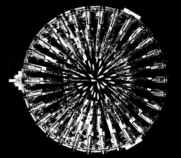
Figure 1: MEFOS general arm display around the one degree field and viewed from above.

Figure 2: Arm tip showing the two spectroscopic fibres (SF) and the associated image fibre bundle (IF).

With this procedure, the objects on which the spectral fibre will be positioned can be seen in advance - contrarily to blind positioning. It is to our knowledge the only such instrument. By analysing the position of the object on the image, in combination with the fixed displacement between the image bundle fibre and the spectral fibre within an arm, a precise offset is determined and the arm sent to the optimal object position. This offset takes care of all imprecision due to the telescope, the instrument and inaccurate coordinates. The poor pointing of the telescope, and the fact that the corrector and the instrument are frequently dismounted, would make blind positioning extremely dangerous. The final positioning accuracy, as measured on stellar sources, is 0.2 arcsec rms.

To avoid any motion between the telescope and the instrument, the guiding is done in the arm environment. A special arm is dedicated for this task. This arm holds a large image conducting optical fibre with a field of view of 1.8 x 2.5 arcmin. To enlarge the field within which a guide star can be selected, this window can be positioned in 3 different (adjacent) positions. The guiding camera is sensitive to V$<19$. Because of this faint magnitude limit, no guide star has to be defined prior to the observations. The guiding fibre can then remain in the outer position at the edge of the field, leaving more space to the positioning of the arms.

In the present stage, the spectral fibres, $135\hbox{$\mu$m}$ in diameter and 21 m long, are going from the prime focus down to the Cassegrain, where the B&C ESO spectrograph is located. This spectrograph is fitted with a F/3 collimator to match the fibre output beam aperture. It has a set of reflection gratings with dispersion range from 2.3 nm/mm to 23.1 nm/mm, and a Tek 512 x 512 thin CCD.

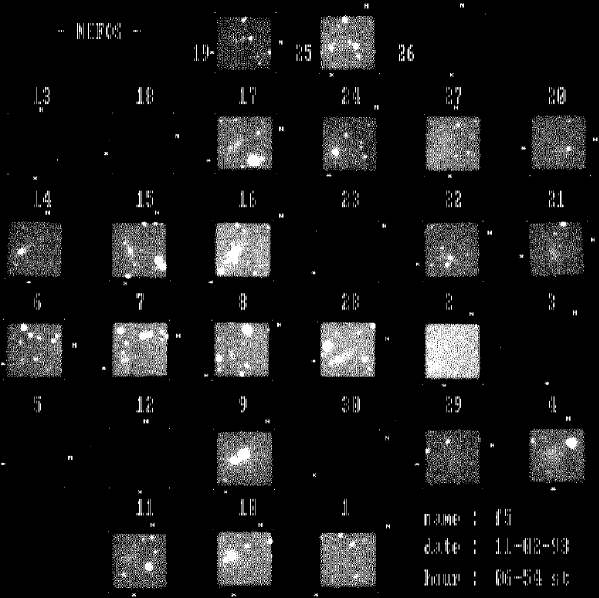
Figure 3: Hardcopy of the monitor screen, showing the sky field recorded by the Peltier cooled CCD of the 30 image fibre bundles after 5 minutes integration. The stars and galaxies are clearly visible.

3 Technical and Scientific Tests on Sky

The first scientific observation was performed in February 1991 with a MEFOS prototype consisting of nine arms only (Bellenger et al. 1991). During this period a galaxy of magnitude B=$18\hbox{$.\!\!^{m}$}6$ was observed with a resolution of R=370. The 1^h exposure resulted in spectrum with a S/N=50 in the red part of the continuum (550 nm).

The first technical run in full configuration at the 3.6m telescope took place in October 1992. As only 2 1/2 of the 5 allocated nights were clear, a second run was necessary for the testing and the commissioning. This was carried out in February 1993 during 5 clear nights. Some problems with the centering of the image fibres on the object coordinates were noted. It appeared that the optical aberrations correction curve was not accurate enough. We had adopted this curve as it was derived from photography at the prime focus. The mounting of this instrument entails different conditions. By moving an image fibre across the MEFOS field in real configuration, the correction curve could be adjusted. The objects are now falling within a few arcseconds of the centre of the image fibre helping for their identification.

In the 7 nights following this run, MEFOS was used on two scientific programmes. The instrument worked well and little time was lost due to technical reasons. Cuby & Mignoli (1994) studied sky subtraction procedures using MEFOS with and without beam switching. They were able to measure redshifts for galaxies with magnitudes as faint as B=22^m from a 90 min exposure (2 x 45 min). A B=$22\hbox{$.\!\!^{m}$}6$ galaxy was observed as well, but the resulting signal to noise ratio of S/N =7 was too low for a reliable redshift measurement.

Since then, MEFOS was used in 84 nights, without a single failure. Since April 1994, MEFOS has been used without any further support from the building team.

4 Observing with MEFOS

In order to compensate the building team of the DAEC for their efforts, 32 nights of guaranteed time were allocated to scientists of this laboratory. From the submitted scientific proposals, four programmes were selected. Each was granted 8 observing nights with MEFOS.

Based on the experience gained in one of these programmes, we describe in the following the preparations before an observing run as well as the typical procedures while observing with MEFOS at the 3.6m telescope. In the next section we will then discuss a number of specific problems that we encountered while reducing the data, and, at the end, a number of examples and some statistics will allow some insight into results that can be expected from multifibre spectroscopy with MEFOS.

The described procedures as well as the obtained data are, of course, strongly related to the selected project. It is therefore important to know some details about the project when discussing the performance of MEFOS. The scientific project “Search in the Galactic Plane toward the Great Attractor” aims at mapping the galaxy distribution in velocity space in the Zone of Avoidance (ZOA) in the general direction of the Cosmic Microwave Background dipole (CMB) and the Great Attractor. Galaxies hidden behind the ZOA are important in derivations of the peculiar motion of the Local Group relative to the CMB , and in explaining the observed streaming (bulk flow) motions, as e.g. in the Great Attractor region. Preliminary scientific results have already been presented (Cayatte et al. 1994, Kraan-Korteweg et al. 1994, 1996a,b). This programme is a continuation of a long-term programme which made use of OPTOPUS, the previous multi-fibre spectrograph of ESO.

4.1 The Scientific Program

A large part of the extragalactic sky is obscured by the Milky Way. To bridge this gap, we have embarked on a search for galaxies behind the Milky Way to the low diameter limit of D=$0\hbox{$.\mkern-4.0mu^{\prime}$}2$ and faint magnitude limit using existing sky surveys (Kraan-Korteweg & Woudt 1994). To date over 10000 previously unknown galaxies were uncovered in the southern Milky Way ($265{{}^{\circ}}\mathrel{\hbox{\hbox to0.0pt{\hbox{\lower 4.0pt\hbox{$\sim$}}\hss}\hbox{$<$}}}\ell\mathrel{\hbox{\hbox to0.0pt{\hbox{\lower 4.0pt\hbox{$\sim$}}\hss}\hbox{$<$}}}335{{}^{\circ}},|b|\mathrel{\hbox{\hbox to0.0pt{\hbox{\lower 4.0pt\hbox{$\sim$}}\hss}\hbox{$<$}}}10{{}^{\circ}}$).

Three observational programmes are ongoing to determine the 3-dimensional distribution of the galaxies detected in the galaxy search: multifibre-spectroscopy in the densest regions, long slit spectroscopy of more isolated galaxies, and HI-observations of fairly large, low surface brightness galaxies. The three approaches are complementary in the depth of the volume they cover and the galaxy population they are optimal for (cf. Kraan-Korteweg et al. 1994, 1995, 1996a).

After using OPTOPUS during 2 observing runs in 1990 and 1992, the multifibre spectroscopy was continued using the guaranteed scientific test time with MEFOS in 1993 (2 1/2 nights), 1994 (4 nights) and 1995 (4 nights).

The magnitudes of the galaxies discovered in the optical search range between $12\hbox{$.\!\!^{m}$}5<B_{J}<20\hbox{$.\!\!^{m}$}5$, with a strong peak $17\hbox{$.\!\!^{m}$}5<B_{J}<19\hbox{$.\!\!^{m}$}5$ (cf. Fig. 1 in Kraan-Korteweg & Woudt, 1994). This range is well suited to the dynamic range of MEFOS. Galaxies in this magnitude interval have an average number density of the order of 100-200 galaxies$/\Box{{}^{\circ}}$, suggesting a more efficient use of OPTOPUS with 50 fibres in a half-degree field. However, the galaxies of this project lie behind the Milky Way. They are heavily obscured: around one magnitude at the border $|b|=\pm 10{{}^{\circ}}$ of our survey, increasing to 5-6 magnitudes towards lower latitudes (close to the Galactic dust equator the galaxies are fully obscured). The average number density for $18^{th}$ magnitude galaxies is therefore considerably lower. In fact, the multifibre capacity of MEFOS with 29 objects per one-degree field in combination with its capability of obtaining good S/N spectra for these faint obscured galaxies of our survey, make it the ideal instrument to trace large-scale structures close to the plane of the Milky Way.

The galaxies of the Zone of Avoidance survey not only are very obscured and often of low surface brightness, but since they are located in the Milky Way, the fields are crowded with foreground stars, many of which are often superimposed on the faint galaxy images. Here, the imaging facility of MEFOS for object identification and optimal centering of the spectral fibre is again a most advantegous property (as for spectroscopy of LSB objects and/or in crowded fields in general).

4.2 Observational Set-Up

4.2.1 Arms to objects allocation

To prepare an observation, it is necessary to have a list of objects with coordinates precessed to the date of observation and known with a precision of the order of one arcsec. Arm-object assignation software is provided which can be obtained by ftp from ESO. This work is optimally done at the home institute before the observing run and does not cost telescope time. The software is also implemented at La Silla, allowing new or optimization of field assignations during the observing run.

The arm assignation software displays the objects of an earlier prepared list on the screen. A circle of one degree (the size of the MEFOS field) can be moved around the screen until optimal centering of the field is attained. The computer then suggests a possible configuration for an arm-object assignation. The software does take the constraints of size and moving capacity of the arms into account, to avoid collisions. The smallest allowed distance between objects depends on the relative arm positions. It lies between 2 and 5.8 arcmin. If the proposed assignation is not optimal from a scientific point of view, it can be modified interactively (within the above named limits). Figure 4 shows an example of an assigned field. The arms are displayed with their true extent.

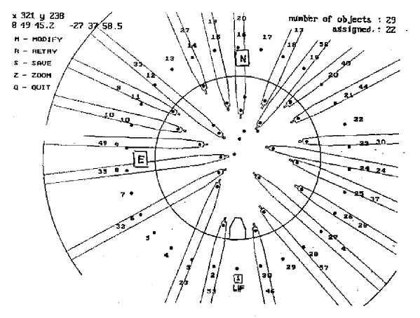
Figure 4: Example of an arm to objects field allocation. The inner circle limits the one degree field. The inner numbers are arm numbers, the outer ones are the object numbers given in the prepared list.

4.2.2 Instrument set-up at the telescope

MEFOS is installed with the corrector at the prime focus. The North-South direction has to be known with a high precision. A set of star fields, equally spaced in right ascension, are used during the set-up for calibration.

The pointing of the telescope is essential when observing with MEFOS. During the set-up, the pointing will be checked in detail. This will lead to a pointing model which is automatically applied during the whole observing run. It is therefore not necessary to recheck the pointing. Any change in the pointing should be avoided, as this will destroy the pointing model. The pointing only has to be rechecked if the system had, for some reason, to be rebooted.

The instrument is focussed by pointing the guiding arm to a star. This fibre has a larger field of view compared to the object image fibres.

4.3 Observational Procedure

4.3.1 Objects acquisition

The telescope is pointed towards the selected field. As soon as the the telescope is locked on the centre of the MEFOS field, the guiding has to be switched on.

There are 3 adjacent guide fields of 1.8x2.3 arcmin each, in which a guide star can be found. The magnitude of the star can be as faint as 19th magnitude. In the exceptional case that no guide star can be found in any of the 3 possible guide field positions, it is better to switch to another target field in order not to lose valuable observing time. An arm-object reassignment to enhance the likelyhood of finding a star in the guiding window can be done at a later point of time. The arms are then sent to their previously assigned object positions, with the image fibre bundles centered on the objects. During the arm positioning, the PC controlling the MEFOS operations, continously displays the movements of the arms. It typically takes about 4 minutes for the arms to reach their final positions. As soon as the arms are in position, a CCD image is taken (see Fig. 3). The images are crucial, because they allow object identification and accurate centering of the spectral fibre. These images are raw and cannot be used for other scientific purposes like photometry. The readout time for the CCD image is 17 sec. The noise is quickly sky dominated. An exposure time for a V=17$.\!\!^{m}$2 star is of the order of 20 sec with 1.7 arcsec seeing. For a B=20^m galaxy, depending on the shape, about 3 min are needed.

We generally exposed as long as 5 or 7 minutes because the objects of our programme are obscured galaxies, often of low surface brightness in fields crowded by foreground stars. The identification of our objects in the 35”x 35” field was therefore often difficult. For brighter objects in less crowded fields the advocated 2 to 3 minutes is adequate.

4.3.2 Object identification

After the images are taken and displayed on the screen, the observer has to identify the object on the respective images for final optimal positioning. This can be done automatically or manually. An internal routine searches for the brightest objects within the images and puts numbered boxes around them. The correct object can then be identified by entering the number of the box into the computer. The optimal position can also be indicated manually by clicking with the cursor on the required position. The latter is a more efficient procedure for centering of very low surface brightness objects. Depending on the number of objects in the field of view and on the surface brightness of the objects, this step takes between 5 and 10 minutes. If the objects are very faint or multiple, it is advisable to make polaroid copies and mark the position where the spectral fibre will be put. It takes about one minute to send the spectroscopic fibres to the recentered objects.

4.3.3 Calibration and scientific exposures

After the identification step, the observing procedure depends on the scientific programme. A flat field with an internal white lamp allows to identify and to check the position of the fibres on the CCD. The exposure time is about 10 sec. The He and Ne lamps are used for the wavelength calibration (note that the Neon lamp has to be requested before the setting). It is recommended to have a filter (BG 28) put in front of the Neon to reduce the intensity of the red Neon lines and avoid saturation. The two lamps can be exposed simultaneously. Based on our experience, an exposure time of about 1 min is reasonable.

Then the scientific exposures can begin. Depending on the programme, magnitude and surface brightness of the objects, a sequence of 30 min exposures follows. With more than two consecutive exposures of one field, another calibration was taken to test the stability of the wavelength calibration.

This whole procedure has to be repeated for every field. The overhead between one scientific exposure of a field to the next field typically takes 20 to 30 min, calibration included. With two observers at the telescope some of these operations can be done simultaneously, saving therewith on ’real’ observing time.

For an exposure time of 2x30 min, 5 to 6 fields per night can be observed depending on the length of the nights. We observed 9 fields in 2 1/2 nights in February 1993, 19 fields in 4 nights in February 1994 and 19 fields in 4 nights in May 1995.

5 Data Reduction

We used the CCD Tek #32 in our observing runs with the grating #15. This resulted in a dispersion of 170Å/mm and a resolution of about 11Å. The wavelength range was chosen to be 3850Å- 6150Å.

The data reduction has been carried out on Sun stations with the IRAF package. The reduction process consists of subtraction of a mean bias, extraction of the spectra, wavelength calibration, fibre transmission correction, sky subtraction, removal of cosmic-ray events and redshift determination. For the last step we used the RVSAO package obtained from the Smithsonian Astrophysical Observatory developed by Doug Mink. With this package, radial velocities can be obtained with the cross-correlation method proposed by Tonry and Davis (1979), and redshifts can also be determined from emission lines if present. In the course of our observing runs, we regularly observed a number of standard velocity stars (1-2 per night) which were subsequently used in the cross-correlation of each object spectrum.

We will not give a detailed description of the various steps of the the reduction process – this will be given in the forthcoming paper on the scientific programme – but rather highlight some specific problems.

5.1 The determination of the spectra position and the wavelength calibration

Efficient extraction of spectra and accurate wavelength calibration are critical in measuring accurate redshifts. This does require deep understanding of the performance of the system such as the illumination of calibration and flat-field sources. In the following we point out some problems that we encountered while reducing the multifibre data.

5.1.1 Extraction and calibration procedure

For each fibre the position of the spectrum on the CCD has to be defined. This is done by measuring the centroid of the profile perpendicular to the dispersion. The curvature in the dispersion direction is corrected by fitting the centroid position for each object as a function of the coordinate along the wavelength axis. The positions of the spectra are determined from a flat field exposure in the same telescope configuration as the objects of the field exposure. No ”cross-talk” between two adjacent spectra has been evidenced, so an extraction window as large as the spectra separation can be chosen. In our case we use an extraction window of 5 pixels for each aperture (adding faint signal in the profile wings reduces the S/N ratio for the object spectrum). Spectra for each aperture in each exposure were then extracted with ”variance” weighting.

The dispersion was determined for each aperture (e.g. each spectrum) from the corresponding aperture on the He-Ne lamp calibration exposures. For the dispersion solution we used 13 emission lines from the He-Ne lamp. We fitted a cubic spline of order 3 to the non-linear component. The residuals were not larger than 0.3Å . By measuring the scatter in the skyline position, we always obtained an uncertainty in the wavelength calibration below 0.5Å (e.g. 30${\,km\ sec^{-1}\,}$).

5.1.2 Flexure and stability

The total flexure between the CCD mounted on the B&C spectrograph (mounted at the Cassegrain focus) and the fiber focus has been checked in both directions. To look for positioning repeatability of the spectra, we have compared two flat field exposures of different telescope pointing. After both the telescope and all arms were moved to other locations, differences between the positions of the spectra for two flat-field exposures were found, though never more than 0.25 pixels (e.g. 7$\mu$m). Flexure with telescope tracking was checked by comparing two flat field exposures taken with the same telescope pointing. The maximum noted flexure in an hour never exceeded 0.25 pixels, i.e. 7$\mu$m.

In the dispersion direction we compared two lamp calibration exposures taken before and after successive field exposures. The 1993 MEFOS run revealed a shift of about 1Å per hour depending on telescope position. This corresponds to a quarter of a pixel, i.e. is of similar order as in the spatial direction. This effect was seen in almost all the fields. It could be due to a continuous drift with time. The February 1994 MEFOS run did not exhibit any such effect.

5.1.3 Positioning and calibrating problems

While reducing the fields of the February 1993 and 1994 runs, we noticed inconsistencies between the positions of the spectra obtained from the flat field as compared to the objects: the difference in position between the flat and the object is roughly constant up to the middle of the CCD frame and then decreases as a function of pixel position in the spatial direction up to -0.5 pixels (e.g. 13$\mu$m). This trend is displayed in Figure 5. Although the mean curves of the different fields are slightly displaced from each other, they all clearly exhibit the same trend. Moreover the mean shift changes as a function of wavelength. It is stronger in the blue part of the image. The problem therefore does not seem related to the mechanical stability and reliability, but rather to the difference in the light path of the lamp used for the flat field exposure and the object exposure. Cuby and Mignoli (1994) noticed displacement problems as well. However, they find a difference between flat-field and sky spectra positions which varies linearly with the centroid of the spectra.

Figure 5: Difference in the position between the flat and the object as a function of pixel position in the spatial direction on the CCD. The different symbols represent six of the fields from the 1993 run.

Because of these difficulties, the MEFOS-user is adviced to check for such systematic effects and not to blindly use the flat fields for defining the spectra positions. To circumvent these problems, we extracted the spectra positions directly from the object spectra. The two exposures per field were summed up if no shift between the positions on the CCD frames could be found. This addition increases the signal to noise ratio in the less sensitive, blue part of the spectra. The errors in the position of the spectra in the faint blue part are of the order of 0.3 pixels (as compared to the FWHM of the spectra profile of about 3 pixels). A large extracting window, on the same order of the spectra separation, will decrease the loss of signal due to the imprecise determination of centroid of the profile.

For certain fibres the spectra were not properly wavelength calibrated. For these spectra the [OI] skyline wavelength position was not close to the actual value of 5577.4Å . So we also checked the alignment of the fibres along the slit by comparing He-Ne lines positions for different apertures; the result is shown in the bottom panel of Fig. 6 : the mean spectral-shift of all the He-Ne lines in the dispersion direction has been plotted versus the aperture position coordinate on the spatial axis. The points seem to be located around a parabola which represents the image of the slit through the spectrograph. In the top panel of Fig. 6 , we have plotted the differences between the measured position of the [OI] skyline and 5577.4Å versus the aperture position coordinate on the spatial axis. The largest displacement of the skyline position occurs for the fibres which are the most misaligned on the slit. As suggested in the previous paragraph, different optical paths for sky and lamp exposure are suspected. Here we observe this effect in the dispersion direction. We cannot wavelength-calibrate the spectra correctly for objects observed with fibres that are located far from the slit center in the spectral direction.

Figure 6: Mean shift of all the He-Ne lines in the dispersion direction as a function of the aperture position in pixels on the other axis (bottom panel). The difference between the measured and the real wavewlength of the [OI] skyline is presented in the top panel.

The optical paths difference could be explained if misaligned fibres have undergone some bending effect or that the plane of the slit (in front of the fibers) is not perfectly perpendicular. This would change the position of the image if the CCD is illuminated by the sky or by a calibration lamp.

To correct the bad wavelength calibration we estimated a mean shift by averaging the [OI] skyline offsets. These were measured from each exposure in a field. We then applied an inverse shift of the corresponding amount to each spectrum taken in the ”misaligned” fibres. The largest discrepancies between measured and actual value was consistently seen for the same fibers in all the 18 observed fields of the 1994 run. The r.m.s error of the mean skyline offset was never larger than 0.17Å . Generally, it was of the order of 0.12Å , corresponding for a wavelength of 5577.4Å to an r.m.s. error of 6${\,km\ sec^{-1}\,}$ in velocity.

5.2 The fibre transmission correction and sky subtraction

We estimated the relative transmission of each fibre from the [OI] 5577.4Å skyline flux to correct the fiber efficiencies. After this correction, we averaged all the sky spectra in a given field. This minimizes the noise of the sky spectrum to be subtracted from the object spectra. With MEFOS, each arm carries its own sky fibre, allowing therewith other sky subtraction methods. Detailed investigations on optimal sky subtraction routines have been performed by Cuby and Mignoli (1994). They find averaging over all sky spectra, after fibre efficiency correction as determined from the skyline flux the best solution. This does of course depend on the programme. For spectrophotometry of galactic or extragalactic objects, for instance, precise flux calibration will be required.

The fibre relative transmission coefficient deduced from the [OI] 5577.4Å skyline flux takes into account the sky variations over the field together with the effective fibre efficiency determination, without the possibility of disentangling the two effects. Generally, sky variation is rather weak below 6000Å  even on a one degree field (see results of Cuby and Mignoli, 1994). The transmission variations observed for some fibres during the night as well as from night to night, could therefore be largely due to a change in fibre efficiency, which can, for instance occur when light injection conditions vary. Nevertheless, the transmission coefficient values obtained from two exposures on the same field show very little scatter. From the statistic on the fibre transmission difference between the two exposures we derived an r.m.s. error on the estimation of this coefficient below 2%.

6 Results

6.1 Objects per field

In 1993 and 1994, 506 objects have been observed on 27 fields. This translates to an average of 19 objects per MEFOS field. This number is considerably lower than the maximum of 29 objects within a one degree circle. On the one hand, this reflects the choice of a field, on the other hand the constraints of the instrument itself. Besides scientific priorities, constraints are given by the arms; i.e. the width of the arm and the minimum allowed distance. The average number of objects that we could observe in crowded fields was of the order of 22 to 24 galaxies. Numbers of 27 to 29 were indeed achieved if the galaxy density reached a hundred or more, as in fields of the cluster Abell 3627 (Kraan-Korteweg et al., 1996a).

6.2 Derived redshifts

Of 473 spectra in 24 reduced fields, redshifts have been obtained for 93% of the objects, among which 84% are of galaxies and 9% are of stars.
The perturbations of the galaxy spectrum by foreground stars (of the 47 spectra contaminated by a superimposed star, only 6 redshifts of galaxies could be obtained) is, of course, a problem inherent to our programme and should not affect observing programmes away from the Galactic Plane. Among the redshifts obtained for galaxies, 77% are reliable (i.e. with a S/N ratio larger than 20 at 5000Å ) with errors in velocities which in the mean are about $60{\,km\ sec^{-1}\,}$. For 22% of the objects, the redshift could be attained from emission lines.

The distribution of the good S/N redshifts are displayed in Fig. 7 for the velocity range of $0<v_{h}<45000{\,km\ sec^{-1}\,}$.

The distribution in Fig. 7 depends strongly on the extragalactic large-scale structures that are being intercepted in the Milky Way. For instance, the strong peak at about $5000{\,km\ sec^{-1}\,}$ mainly stems from 4 MEFOS fields centered on the cluster A3627 at $(\ell,b)\approx(325{{}^{\circ}},-7{{}^{\circ}})$. The velocities from these 4 fields are marked by the dashed histogram. In fact, the velocities from these observations, in combination with the result from our complementary observations at the SAAO and at Parkes, have proven this cluster to be very massive and therefore to be at the bottom of the potential well of the Great Attractor (Kraan-Korteweg et al. 1996a).

Figure 7: Distribution of the 334 redshifts obtained from observations with MEFOS in 1993 and 1994 from good S/N spectra. The dashed histogram is a subsample of 4 fields centered on A3627, a massive cluster close to the core of the Great Attractor.

The mean velocity of the observed sample is $<v_{h}>=16500{\,km\ sec^{-1}\,}$. The peaks at 12000, 18000 and 23000${\,km\ sec^{-1}\,}$ are part of filaments that diagonally cross the Zone of Avoidance. They can be traced to higher latitudes on both sides of the Milky Way and are indicative of extragalactic large-scale structures of considerable size (a few hundred Mpc). For further details see Kraan-Korteweg et al. (1994 & 1996b).

Figure 8: Magnitude distribution of the galaxies for which redshifts have been determined from a 2x30 min exposure with MEFOS. The histogram reflects the magnitude distribution of the galaxy sample rather than a constraint of the instrument MEFOS. This can be seen from the interior dashed histogram which are galaxies for which no redshift could be determined because of low S/N ratio.

Here, it suffices to maintain that MEFOS produces good quality spectra for galaxies as distant as $45000{\,km\ sec^{-1}\,}$ .

6.3 Dependence on magnitude and mean surface brightness

The above results do depend on the properties of the observed galaxies like the magnitude and the mean surface brightness, although the best parameter would be the central surface brightness corresponding to the flux collected at the position of the fiber. One can imagine a very low mean surface brightness galaxy with a relatively bright nucleus, giving a good S/N spectrum.

In Fig. 8 the distribution of the apparent magnitudes B_J of 361 galaxies with redshifts is displayed. The magnitudes are estimates from the IIIaJ film copies of the SRC. Although eye estimates, it has been shown that these magnitudes are accurate to $\sigma=0\hbox{$.\!\!^{m}$}5$ with no deviations from linearity up to the faintest galaxies. (cf. Kraan-Korteweg and Woudt, 1994, Kraan-Korteweg 1996).

The mean magnitude of the observed galaxy sample is $<B_{J}>=17\hbox{$.\!\!^{m}$}8$. If this distribution is compared to the one of the galaxies for which no redshift could be extracted (dashed histogram in Fig. 8), no clear bias is visible toward the faintest objects. Therefore the derivation of a redshift in this magnitude range does not critically depend on magnitude. The distribution shows a strong peak between $17\hbox{$.\!\!^{m}$}5$ and $19\hbox{$.\!\!^{m}$}0$ which does reflect the magnitude distribution of the Galactic Plane survey (cf. Fig. 1 in Kraan-Korteweg & Woudt, 1994).
A slightly stronger dependence has been noted with mean surface brightness $SB_{J}$. The mean surface brightness ranges between $22\hbox{$.\!\!^{m}$}8\leq SB_{J}\leq 24\hbox{$.\!\!^{m}$}5$ with a narrow Gaussian distribution around $<SB_{J}>=23\hbox{$.\!\!^{m}$}5$ ($\sigma=0\hbox{$.\!\!^{m}$}29$), whereas the galaxies for which no redshift could be determined have a mean of $<SB_{J}>=23\hbox{$.\!\!^{m}$}8$ ($23\hbox{$.\!\!^{m}$}3\leq SB_{J}\leq 24\hbox{$.\!\!^{m}$}1$). But a redshift could be derived for the faintest few galaxies as well as for the one with the lowest surface brightness.

A weak correlation between velocity and surface brightness was noted: while the galaxies with $v<30000km/s$ show a stable distribution about the mean, the galaxies with $v>30000{\,km\ sec^{-1}\,}$ reveal a decrease in mean surface brightness with increasing redshift.
In Figure 9, a few characteristic examples of galaxies from our survey and their resulting spectrum from a 2x30 min exposure with MEFOS are shown. They illustrate the quality of the obtained spectra as a function of the properties of the observed galaxies and visualize the above discussed tendencies. Three of the four objects presented in Fig. 9 have a $B_{J}$ magnitude nearly equal to the mean one of the whole sample, but the mean surface brightness spans a large range. The object shown in the lower-left panel is one of the faintest galaxy of our sample, a 20^th-magnitude spiral galaxy with a very low mean surface brightness ($SB_{J}=24\hbox{$.\!\!^{m}$}1$). The CCD images of the galaxies clearly show that the central surface brightness is the most important factor in achieving a high S/N ratio. The velocities of the two objects in the upper panels are of the order of the mean velocity obtained for the sample, but the galaxies in the lower panels are more distant.

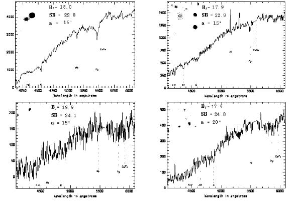
Figure 9: Spectra of four galaxies observed with MEFOS. The 0’.5x0’.5 CCD images is shown above each spectra. Their magnitude B_J, mean surface brightness and diameter are indicated.

¿From the overall analysis of the observed sample, it can be maintained that good signal to noise spectra can be obtained with MEFOS from 2x30 min exposures for galaxies up to a magnitude of $B_{J}\leq 19\hbox{$.\!\!^{m}$}5-20\hbox{$.\!\!^{m}$}0$, the approximate magnitude limit of our survey. For these obscured galaxies behind the Milky Way, we have measured redshifts of galaxies up to $v_{h}<45000{\,km\ sec^{-1}\,}$. Reliable redshifts can be expected for a percentage of over $\mathrel{\hbox{\hbox to0.0pt{\hbox{\lower 4.0pt\hbox{$\sim$}}\hss}\hbox{$>$}}}90\%$. This efficiency does depend on surface brightness and, especially in the case of this programme, is limited by interfering foreground stars, an effect which would be much stronger were it not for the imaging capability of MEFOS.

7 Conclusions

In this paper we present the features of MEFOS, a multi-object fibre positioner coupled to the B&C spectrograph and implemented at the prime focus of the ESO 3.6 m Telescope at La Silla. This instrument is open to the ESO community and was used on the sky for 84 nights, until now. MEFOS is an arm type instrument which is able to position 29 fibres on designed targets and has the same number of sky fibres. Very precise fibres positioning with this instrument is only possible on this generation of telescopes with a vision system that is associated to the arms. MEFOS aim is the observation of moderately crowded fields that need a one degree field for efficient observations.

Several scientific programmes have been conducted with MEFOS. The results obtained for one of them, aiming at measuring redshifts of galaxies found in the Galactic Plane, is given as an example of what can be observed with MEFOS, and what were the encountered problems with the data reduction.