Abstract

We present an analysis of CMB anisotropies induced by global scalar fields in the large $N$ limit. In this limit, the CMB anisotropy spectrum can be determined without cumbersome 3D simulations. We determine the source functions and their unequal time correlation functions and show that they are quite similar to the corresponding functions in the texture model. This leads us to the conclusion that the large $N$ limit provides a ’cheap approximation’ to the texture model of structure formation.

PACS numbers: 98.80.Cq 98.65.Dx

The anisotropies in the cosmic microwave background (CMB) have become an extremely valuable tool for cosmology. There are hopes that the measurements of the CMB anisotropy spectrum might lead to a determination of cosmological parameters like $\Omega_{0},~{}H_{0},~{}\Omega_{B},~{}\Lambda$ to within a few percent. The justification of this hope lies to a big part in the simplicity of the theoretical analysis. Fluctuations in the CMB can be determined almost fully within linear cosmological perturbation theory and are not severely influenced by nonlinear physics.

Presently there are two competing classes of models which lead to a Harrison Zel’dovich spectrum of fluctuations: Perturbations may be induced during an inflationary epoch or they may be due to scaling seeds like, e.g., a self ordering global scalar field or cosmic strings (for a general definition of ’scaling seeds’ see [1]). In the first class, the linear perturbation equations are homogeneous. In the second class they are inhomogeneous, with a source term due to the seed. The evolution of the seed is in general non–linear and complicated and therefore much less accurate predictions have been made so far for models where perturbations are induced by seeds.

In this communication we discuss an especially simple model with seeds where the equation of motion for the seed perturbations can be solved explicitly. We consider a $N-$component real scalar field $\phi$ with $O(N)$ symmetric potential $V$, which at $T=0$ is given by $V=\lambda(\phi^{2}-\eta^{2})^{2}$. At low temperatures, $T\ll\eta$, $\phi$ can be regarded as constrained to an $N-1$ sphere with radius $\eta$. The scalar field then evolves according to the non–linear $\sigma$–model which is entirely scale free. In terms of the dimension-less variable $\beta=\phi/\eta$ we find

$$\Box\beta-(\beta\cdot\Box\beta)\beta=0~{},$$ (1)

with the condition $\beta^{2}=1$. The non–linearity in this equation, $-(\beta\cdot\Box\beta)\beta=(\partial_{\mu}\beta\cdot\partial^{\mu}\beta)\beta$ contains a sum over $N$ components. In the limit $N\rightarrow\infty$, this sum can be replaced by an ensemble average and the resulting linear equation of motion can be solved exactly. One obtains [2]

$$\beta(\vec{k},t)=At^{\frac{3}{2}}\frac{J_{\nu}(kt)}{(kt)^{\nu}}\beta_{in}(\vec{k}).$$ (2)

The index $\nu$ is determined by the background matter model and varies between $\nu=2$ in a radiation dominated background and $\nu=3$ in a matter dominated background. The pre-factor $A$ is chosen to ensure $\beta^{2}=1$,

$$A=\left\{\begin{array}[]{ll}15/16,&\mbox{if }\nu=2,\\ 2835/128,&\mbox{if }\nu=3.\end{array}\right.$$

The components of $\beta_{in}$ are assumed to be independent, Gaussian-distributed random variables with vanishing mean and dispersion $\langle(\beta_{in})_{j}^{2}\rangle=1/N$ for all values of $j$. (Clearly, the variables $(\beta_{in})_{j}$ cannot be completely independent, since they obey the condition $\sum_{j}(\beta_{in})_{j}^{2}=1$.)

Once the scalar field $\beta$ is known, we can calculate its energy–momentum tensor, the induced gravitational field and and its action on matter and radiation within linear cosmological perturbation theory. As has been discussed in [2], the energy density of a four component global scalar field is already quite close to the large $N$ limit and there are thus justified hopes, that this simple model might provide a quite sensible approximation to the texture scenario for structure formation. On the other hand, we know that non–linearities, which lead to the mixing of scales and to the deviations from a Gaussian distribution, are crucial for some qualitative properties of defect models, like decoherence [3, 1]. In the large$-N$ limit, the only non–linearities are the quadratic expressions of the energy momentum tensor, and thus effects like decoherence might be mildened substantially in this model.

This communication is an outline of a longer paper in preparation. We first briefly repeat the basic equations for the determination of the CMB anisotropy spectrum in the presence of seeds, and solve the equations (for given seed functions) in a simplified situation. We then outline the calculation of the relevant correlation functions and present some results. We end with conclusions and an outlook.

The coefficients of the angular power spectrum of CMB anisotropies are related to the 2–point function according to [5]

$$\left.\left<\frac{\delta T}{T}(\vec{n})\frac{\delta T}{T}(\vec{n}^{\prime})\right>\right|_{(\vec{n}\cdot\vec{n}^{\prime}=\cos\varphi)}=\frac{1}{4\pi}\sum_{\ell}(2\ell+1)C_{\ell}P_{\ell}(\cos\theta)~{}.$$ (3)

For pure scalar perturbations, neglecting Silk damping, the $C_{\ell}$’s are given by[1]

$$C_{\ell}=\frac{2}{\pi}\int\frac{\left<\left|\Delta_{\ell}(\vec{k})\right|^{2}\right>}{(2\ell+1)^{2}}k^{2}dk$$ (4)

where

$$\frac{\Delta_{\ell}}{2\ell+1}=\frac{1}{4}\Delta_{gr}(\vec{k},t_{\mbox{\scriptsize dec}})j_{\ell}(kt_{0})-V_{r}(\vec{k},t_{\mbox{\scriptsize dec}})j_{\ell}^{\prime}(kt_{0})+k\int_{t_{d\!e\!c}}^{t_{0}}(\Psi-\Phi)(\vec{k},t^{\prime})j_{\ell}^{\prime}(k(t_{0}-t^{\prime}))dt^{\prime}.$$ (5)

For large $\ell$ this spectrum is corrected by Silk damping, which can be approximated by multiplying $\Delta_{\ell}(k)$ with an exponential damping envelope [4].

We want to consider the situation where fluctuations are induced by seeds. We restrict ourselves to scalar perturbations. The energy momentum tensor of scalar seed perturbations can be parameterized by the following four functions: $f_{\rho}$ the energy density of the seed, $f_{p}$ the pressure of the seed, $f_{v}$ a potential for the energy flux of the seed and $f_{\pi}$ the potential for anisotropic stresses of the seed [6, 7] (see below). The linear cosmological perturbation equations are then of the form

$${\cal D}X_{j}=M_{j}^{i}F_{i}~{},$$ (6)

where ${\cal D}$ is a first order linear differential operator, $X$ is a vector consisting of all, say $m$, gauge invariant perturbation variables of the cosmic fluids (like $\Delta_{gr}$, $V_{r}$, and, e.g. the corresponding variables for the cold dark matter (CDM), …). $F=(f_{\rho},f_{p},f_{v},f_{\pi})$ is the source vector and $M$ is a, in general time dependent, $m\times 4$ matrix.

The general solution to Eq. (6) is of the form

$$X_{j}(t)=\int_{t_{in}}^{t}G_{j}^{i}(t,t^{\prime})F_{i}(t^{\prime})dt^{\prime}~{},$$ (7)

where $G$ is the Green’s function of the differential operator $\cal D$. The Bardeen potentials $\Phi$ and $\Psi$ are algebraic combinations of the fluid variables $X_{j}$ and the source functions $F_{i}$,

$$(\Psi-\Phi)(t)=P^{j}(t)X_{j}(t)+Q^{i}(t)F_{i}(t)~{}.$$ (8)

Inserting this solution in Eq. (5) we obtain

$${\Delta_{\ell}\over 2\ell+1} = \int_{t_{in}}^{t_{dec}}dt\left[{1\over 4}G_{\Delta_{r}}^{i}(t_{dec},t)j_{\ell}(kt_{0})-G_{V_{r}}^{i}(t_{dec},t)j^{\prime}_{\ell}(kt_{0})\right]F_{i}(t)$$ (9)

$$+k\int_{t_{dec}}^{t_{0}}dt\left[\int_{t_{in}}^{t}dt^{\prime}(P^{j}(t)G_{j}^{i}(t,t^{\prime})F_{i}(t^{\prime}))~{}+~{}Q^{i}(t)F_{i}(t)\right]~{}.$$

The expectation value in Eq. (4) thus consists of time integrals of unequal time correlations of the source functions, which are of the generic form

$${\langle|\Delta_{\ell}|^{2}\rangle\over(2\ell+1)^{2}} = \int^{t_{dec}}_{t_{in}}dt\int^{t_{dec}}_{t_{in}}dt^{\prime}\langle F_{i}(t)F_{j}(t^{\prime})\rangle A_{\ell}^{ij}(t,t^{\prime})~{}+~{}$$ (10)

$$~{}+~{}\int_{t_{dec}}^{t_{0}}dt\int_{t_{dec}}^{t_{0}}dt^{\prime}\int_{t_{in}}^{t}dt^{\prime\prime}\int_{t_{in}}^{t^{\prime}}dt^{\prime\prime\prime}\langle F_{i}(t^{\prime\prime})F_{j}(t^{\prime\prime\prime})\rangle B_{\ell}^{ij}(t,t^{\prime},t^{\prime\prime},t^{\prime\prime\prime})~{}+~{}$$

$$~{}+~{}\int_{t_{dec}}^{t_{0}}dt^{\prime}\int_{t_{dec}}^{t_{0}}dt\int_{t_{in}}^{t}dt^{\prime\prime}\langle F_{i}(t^{\prime})F_{j}(t^{\prime\prime})\rangle C_{\ell}^{ij}(t,t^{\prime},t^{\prime\prime})~{}+~{}$$

$$~{}+~{}\int^{t_{dec}}_{t_{in}}dt^{\prime}\int_{t_{dec}}^{t_{0}}dt\int_{t_{in}}^{t}dt^{\prime\prime}\langle F_{i}(t^{\prime})F_{j}(t^{\prime\prime})\rangle D_{\ell}^{ij}(t,t^{\prime},t^{\prime\prime})~{}+~{}$$

$$~{}+~{}\int_{t_{dec}}^{t_{0}}dt\int_{t_{dec}}^{t_{0}}dt^{\prime}\langle F_{i}(t)F_{j}(t^{\prime})\rangle E_{\ell}^{ij}(t,t^{\prime})~{}+~{}$$

$$~{}+~{}\int_{t_{dec}}^{t_{0}}dt\int^{t_{dec}}_{t_{in}}dt^{\prime}\langle F_{i}(t)F_{j}(t^{\prime})\rangle H_{\ell}^{ij}(t,t^{\prime})~{}.$$

To calculate the $C_{\ell}$’s we need therefore need to know the unequal time correlations of the seed functions $F_{i}$ and the Green’s functions for the cosmological model specified. In general this is a quite formidable task. Here we shall just discuss a toy model. A somewhat more complicated example is given in [3].

We consider a pure radiation universe with vanishing spatial curvature. In this case, the linear perturbation equations are given by [7]

$$\Phi = \frac{1}{x^{2}+6}\left(x^{2}\Phi_{S}+\frac{3}{2}\Delta_{gr}+6\frac{V_{r}}{x}\right)$$ (11)

$$\Psi = -\Phi-2\epsilon f_{\pi}$$ (12)

$$\Delta_{gr}^{\prime} = -\frac{4}{3}V_{r}$$ (13)

$$V_{r}^{\prime} = \Psi-\Phi+\frac{1}{4}\Delta_{gr}$$ (14)

where $x=kt$ and a prime denotes a derivative w.r.t $x$. The energy momentum tensor of the source enters via the combinations $f_{\pi}$ and $\Phi_{S}=\epsilon(f_{\rho}/k^{2}+3f_{v}/(kx))$. These equations can be combined to a second order differential-equation for $\Delta_{gr}$ alone,

$$\Delta_{gr}^{\prime\prime}+\frac{12}{x^{2}+6}\frac{\Delta_{gr}^{\prime}}{x}+\frac{1}{3}\frac{x^{2}-6}{x^{2}+6}\Delta_{gr}=\frac{8}{3}\left(\epsilon f_{\pi}+\frac{x^{2}}{x^{2}+6}\Phi_{S}\right)~{},$$ (15)

with homogeneous solutions

$$D_{1}(x)=\cos\left(\frac{x}{\sqrt{3}}\right)-2\frac{\sqrt{3}}{x}\sin\left(\frac{x}{\sqrt{3}}\right)~{},~{}~{}D_{2}(x)=-\sin\left(\frac{x}{\sqrt{3}}\right)-2\frac{\sqrt{3}}{x}\cos\left(\frac{x}{\sqrt{3}}\right)~{},$$

leading to the Greens function

$$G(x,x^{\prime})={\sqrt{3}x^{\prime}\over x(6+x^{\prime 2})}\left[(12+xx^{\prime})\sin({x-x^{\prime}\over\sqrt{3}})+2\sqrt{3}(-x+x^{\prime})\cos({x-x^{\prime}\over\sqrt{3}})\right]~{}.$$ (16)

On super-horizon scales ($x\ll 1$) the solutions of the homogeneous equations consist of one constant and one decaying, $\propto 1/x$, mode, while for $x\gg 1$ we obtain two oscillating modes. The general solution with source term $S(x)$ and initial condition $\Delta_{gr}(0)=V_{r}(0)=0$ is

$$\Delta_{gr}(x) = \int_{0}^{x}G^{1}(x,x^{\prime})S(x^{\prime})dx^{\prime}$$ (17)

$$V_{r}(x) = \int_{0}^{x}G^{2}(x,x^{\prime})S(x^{\prime})dx^{\prime}~{}~{}~{}\mbox{ where}$$ (18)

$$G^{1}=G G^{2}=-{3\over 4}{dG\over dx}~{}.$$ and (19)

Together with Eq. (11) and (12) it is now straight forward to determine the integral kernels A,B,C,D,E and H and thus, for given source correlation functions, the $C_{\ell}$’s.

Let us therefore discuss the source correlation functions of scalar field sources in the large $N$ limit. The seed functions are given by [7]:

$$f_{\rho}=F_{1} = \frac{1}{2}\left[\dot{\beta}^{2}+(\nabla\beta)^{2}\right]$$ (20)

$$f_{p}=F_{2} = \frac{1}{2}\left[\dot{\beta}^{2}-\frac{1}{3}(\nabla\beta)^{2}\right]$$ (21)

$$f_{v}=F_{3} = \Delta^{-1}\left[\dot{\beta}\cdot\beta_{,j}\right]^{,j}$$ (22)

$$f_{\pi}=F_{4} = \frac{3}{2}\Delta^{-2}\left[\beta_{,i}\cdot\beta_{,j}-\frac{1}{3}\delta_{ij}(\nabla\beta)^{2}\right]^{,ij}$$ (23)

Using the fact that the initial fields are uncorrelated and Gaussian distributed,

$$\left<\beta_{i}(\vec{k})\beta_{j}(\vec{p})\right>=\frac{1}{N}\delta_{ij}\delta(\vec{k}+\vec{p})$$ (24)

and using the exact solution Eq. (2) we find the power spectra and the unequal time correlation functions of the seed variables $F_{i}$. Below we give explicit expressions for the power spectra of $f_{\rho}~{},f_{v}$ and $f_{\pi}$ and, as an example, the unequal time correlation function for $f_{v}$. These integrals can be evaluated numerically, examples of which are shown in Figs. 1 and 2. We define $\vec{x}=t\vec{k}$ and we set

$$\chi(x)\equiv\frac{J_{\nu}(x)}{x^{\nu}}~{},~{}~{}~{}\varphi(x)\equiv{3\over 2}\chi(x)-\frac{J_{\nu+1}(x)}{x^{\nu-1}}~{}.$$ (25)

Using these abbreviations we obtain the somewhat cumbersome expressions

$$\left<f_{\rho}(\vec{k},t)\cdot f_{\rho}(\vec{k}^{\prime},t)\right>=$$ (26)

$$\frac{A^{2}}{t}\frac{\delta(\vec{k}+\vec{k}^{\prime})}{2N}\int d^{3}\!y\left\{\varphi(y)^{2}\varphi(|\vec{y}-\vec{x}|)^{2}+\left[\vec{y}(\vec{x}-\vec{y})\right]^{2}\chi(y)^{2}\chi(|\vec{y}-\vec{x}|)^{2}\right.~{},$$

$$\left.-2\vec{y}(\vec{x}-\vec{y})\varphi(y)\varphi(|\vec{y}-\vec{x}|)\chi(y)\chi(|\vec{y}-\vec{x}|)\right\}$$

$$\left<f_{v}(\vec{k},t)\cdot f_{v}(\vec{k}^{\prime},t)\right>=$$ (27)

$$A^{2}t\frac{\delta(\vec{k}+\vec{k}^{\prime})}{N}\int d^{3}\!y\frac{\vec{x}(\vec{x}-\vec{y})}{x^{4}}\varphi(y)\chi(|\vec{y}-\vec{x}|)$$

$$\left[\vec{x}(\vec{x}-\vec{y})\varphi(y)\chi(|\vec{x}-\vec{y}|)+\vec{x}\vec{y}\varphi(|\vec{x}-\vec{y}|)\chi(y)\right]~{},$$

$$\left<f_{\pi}(\vec{k},t)\cdot f_{\pi}(\vec{k}^{\prime},t)\right>=$$ (28)

$$A^{2}t^{3}\frac{9\delta(\vec{k}+\vec{k}^{\prime})}{2N}\int d^{3}\!y\frac{\left[(\vec{x}\vec{y})(x^{2}-\vec{x}\vec{y})+\frac{1}{3}x^{2}(y^{2}-\vec{x}\vec{y})\right]^{2}}{x^{8}}\chi(y)^{2}\chi(|\vec{x}-\vec{y}|)^{2}~{},$$

$$\left<f_{v}(\vec{k},t)\cdot f_{v}(-\vec{k}^{\prime},t^{\prime})\right>=$$ (29)

$$\frac{A^{2}t}{N}\frac{r^{2}}{x^{4}}\delta(\vec{k}-\vec{k}^{\prime})\int d^{3}y\left\{\left[x^{2}-\vec{x}\vec{y}\right]^{2}\varphi(y)\chi(|\vec{x}-\vec{y}|)\varphi(yr)\chi(|\vec{x}-\vec{y}|r)\right.$$

$$+\left.\left[(x^{2}-\vec{x}\vec{y})(\vec{x}\vec{y})\right]\varphi(y)\chi(|\vec{x}-\vec{y}|)\varphi(|\vec{x}-\vec{y}|r)\chi(yr)\right\}~{},$$

where we have set $r=t^{\prime}/t$ in the last equation. The behavior of these functions on very large and very small scales can be obtained analytically. On super horizon scales, $x\rightarrow 0$, the power spectra for $f_{\rho}~{},~{}f_{p}$ and $f_{v}$ behave like white noise. Numerically we have found

$$\left<|f_{\rho}|^{2}\right> {\rightarrow}_{x\rightarrow 0} {1\over Nt}\cdot\left\{\begin{array}[]{rc}9.36\cdot 10^{-2}&\nu=2\\ 10.31\cdot 10^{-2}&\nu=3\end{array}\right.$$ (32)

$$\left<|f_{p}|^{2}\right> {\rightarrow}_{x\rightarrow 0} {1\over Nt}\cdot\left\{\begin{array}[]{rc}1.066\cdot 10^{-2}&\nu=2\\ 0.805\cdot 10^{-2}&\nu=3\end{array}\right.$$ (35)

$$\left<|f_{v}|^{2}\right> {\rightarrow}_{x\rightarrow 0} {t\over N}\cdot\left\{\begin{array}[]{rc}0.8687\cdot 10^{-2}&\nu=2\\ 0.4694\cdot 10^{-2}&\nu=3\end{array}\right.$$ (38)

From general arguments [3, 1], we would have expected also $f_{\pi}$ to behave like white noise on super–horizon scales. However, from Eq. (28) we find that $f_{\pi}$ diverges at small $x$ like $1/x^{2}$. Even though we do not quite understand this result, it does not lead to divergent Bardeen potentials, if we allow for anisotropic stresses in the matter (like e.g. from a component of massless neutrinos). In this case it can be shown [1] that compensation arranges the anisotropic stresses in the fluid, $p\Pi$, such that $f_{\pi}+p\Pi\propto x^{2}f_{\pi}$. Therefore, also the anisotropic stresses contribute a white noise component to the Bardeen potentials on super-horizon scales, namely:

$$x^{4}\left<|f_{\pi}|^{2}\right>{\rightarrow}_{x\rightarrow 0}{t^{3}\over N}\cdot\left\{\begin{array}[]{rc}5.169\cdot 10^{-2}&\nu=2\\ 6.539\cdot 10^{-2}&\nu=3\end{array}\right.$$ (40)

In the limit $x\rightarrow\infty$ the source functions decay like

$$\left<|f_{\rho}|^{2}\right>~{},~{}~{}\left<|f_{p}|^{2}\right> {\rightarrow}_{x\rightarrow\infty} {x^{1-2\nu}\over Nt}$$ (41)

$$\left<|f_{v}|^{2}\right> {\rightarrow}_{x\rightarrow\infty} {x^{-1-2\nu}t\over N}$$ (42)

$$\left<|f_{\pi}|^{2}\right> {\rightarrow}_{x\rightarrow\infty} {x^{-3-2\nu}t^{3}\over N}$$ (43)

In Fig. 1 we plot $t<|f_{\rho}|^{2}>(x)$ as obtained from Eq. (26), and compare it to the corresponding function found by 3D simulations of the texture model.

The normalized unequal time correlation functions are defined by

$$C_{i}(k,t,t^{\prime})={\langle f_{i}(k,t)f^{*}_{i}(k,t^{\prime})\rangle\over\sqrt{\langle|f_{i}(k,t)|^{2}\rangle\langle|f_{i}(k,t^{\prime})|^{2}\rangle}}$$ (45)

In the large $N$ limit, the correlation functions decay like power laws. For $r\equiv t^{\prime}/t$ we find in the limit $r\gg 1~{},~{}kt^{\prime}\gg 1$ the behavior $C_{i}\propto r^{-\gamma_{i}}$, with

$$\gamma_{\rho}=3/2~{},~{}~{}\gamma_{p}=3/2~{},~{}~{}\gamma_{v}=3/2~{},~{}~{}\gamma_{\pi}=5/2~{}.$$ (46)

It is not quite clear to us, whether this behavior is reproduced in the texture model. Due to the arguments given at the beginning, it may well be that $N=4$ and $N\rightarrow\infty$ show a different decoherence behavior. Originally (taking into account the numerical accuracy of about 10% of the 3D simulations) we approximated the decoherence in the texture model with an exponential decay law. However, comparing the unequal time correlation functions for $\dot{\beta}^{2}$ shown in Figs. 2 and 3 for the large $N$ limit and a 3D simulation of the texture model respectively, we realize, that they agree extremely well in the numerically most reliable, central region, and the seemingly stochastic higher order oscillations also found in the texture model might actually be real (see Fig. 4), leading to power law decoherence.

Using these source functions, we have determined the CMB anisotropy spectrum induced by the large $N$ limit of a self ordering scalar field for a spatially flat cosmological model with CDM, radiation and baryons. Since decoherence is so weak for large $N$, we used the approximation of perfect coherence, $C_{i}\equiv 1$. This simplification has been used so far for all ’analytic approximations’ of $O(N)$ models and, e.g., in the case of textures, $N=4$, it seems to agree reasonably with numerical simulations [8]. This will certainly be even more so in the large $N$ limit. The influence of decoherence on the CMB power spectrum is discussed in [3].

We have shown that the large $N$ limit of global scalar fields provides a model of seeded structure formation where CMB anisotropies can be determined without cumbersome numerical simulations and thus with much higher accuracy and large dynamical range at relatively modest costs. Determining the correlation functions of the seed variables just requires numerical convolution of Bessel functions multiplied with powers. Once the seed correlation functions are known, perturbations in matter and radiation can be calculated by solving a system of linear perturbation equations, very similar to the homogeneous case of inflationary perturbations.

We believe that the large $N$ limit has many features in common with the texture model of structure formation and thus provides a “cheap approximation” to this model. The most obvious difference between the analytic limit and the texture model is the decoherence behavior. In the large $N$ limit, the field evolution is linear and non–linearities, which are responsible for decoherence, enter only via the quadratic expressions of the energy momentum tensor. We thus expect decoherence to be somewhat weaker in the large $N$ limit.

In a forthcoming paper, we plan to work out the large $N$ limit in more detail, and to study the dependence of the resulting CMB anisotropy spectrum of cosmological parameters. We also want to investigate more fully the comparison of the large $N$ source functions with the source functions found in 3D simulations of the texture model. The limit discussed here provides an very useful toy model for structure formation with scaling seeds for which decoherence is not important.

Figure 1: The source function $f_{\rho}$: In the large $N$ limit (full line), the approximation used to calculate the $C_{\ell}$’s in Fig. 5 (dashed line) and from a 3 dimensional numerical computation (dot-dashed line) for the texture model ($N=4$).

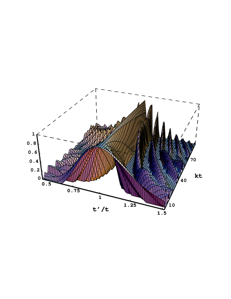
Figure 2: The unequal time correlation function for $\dot{\beta}^{2}=f_{\rho}+3f_{p}$ at fixed $t$ as function of $t^{\prime}$ and $k$ in the large $N$ limit. Negative values are set to zero.

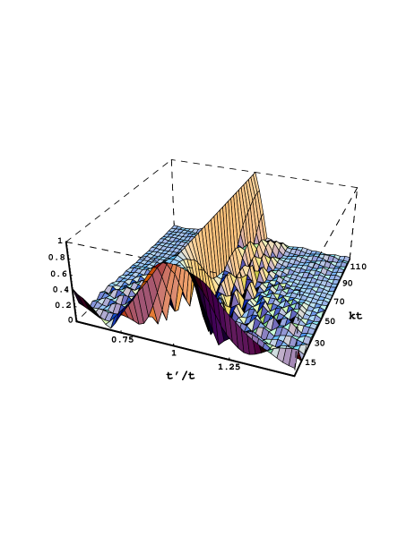
Figure 3: The same as Fig. 2 for the texture model. The similarity is obvious. The high order oscillations which are very pronounced in the large $N$ limit are washed out or absent in the texture model. Whether this is a real feature or just numerical inaccuracy or both is not yet clear.

Figure 4: A cut through Fig. 2 (solid line) and Fig. 3 (dashed line) at $kt=3.9$. The central peaks are in very good agreement. Secondary peaks do not agree and the decay law for the texture model is difficult to predict from this data.

Figure 5: The CMB anisotropy spectrum, obtained by using polynomial fits for the source functions as shown in Fig. 1. Only scalar perturbations are included. The Sachs Wolfe part is indicated by the dotted line, the dashed line represents the acoustic contributions. Silk damping is not included.

References

[1]R. Durrer, M. Sakellariadou and M. Kunz, in preparation (1996).
[2]N. Turok and D. Spergel,
Phys. Rev. Lett.66, 3093 (1991).
[3]J. Magueijo, A. Albrecht, P. Ferreira and D. Coulson,
preprint, archived under astro-ph/9605047 (1996).
[4]W. Hu and N. Sugiyama, “Small scale cosmological perturbations:
an analytic approach”, astro-ph/9510117 (1996).
[5]T. Padmanabhan, Structure Formation in the
Universe, Cambridge University Press (1993).
[6]R. Durrer, Phys. Rev.D42, 2533 (1990).
[7]R. Durrer,
Fund. of Cosmic Physics15, 209, (1994).
[8]N. Turok, Preprint, archived under astro-ph/9600687.