The Stellar Dynamics of $\omega$ Centauri

Abstract

The stellar dynamics of $\omega$ Centauri  are inferred from the radial velocities of 469 stars measured with CORAVEL (Mayor et al. (1997)). Rather than fit the data to a family of models, we generate estimates of all dynamical functions nonparametrically, by direct operation on the data. The cluster is assumed to be oblate and edge-on but mass is not assumed to follow light. The mean motions are consistent with axisymmetry but the rotation is not cylindrical. The peak rotational velocity is $7.9$ km s^-1 at $\sim 11$ pc from the center. The apparent rotation of $\omega$ Centauri  is attributable in part to its proper motion. We reconstruct the stellar velocity ellipsoid as a function of position, assuming isotropy in the meridional plane. We find no significant evidence for a difference between the velocity dispersions parallel and perpendicular to the meridional plane. The mass distribution inferred from the kinematics is slightly more extended than, though not strongly inconsistent with, the luminosity distribution. We also derive the two-integral distribution function $f(E,L_{z})$ implied by the velocity data.

Rutgers Astrophysics Preprint Series No. 205

1 Introduction

Since the mid-1960’s, the standard method for analyzing globular cluster data has been a “model-building” approach (King (1966); Gunn & Griffin (1979)). One begins by postulating a functional form for the phase-space density $f$ and the gravitational potential $\Phi$; often the two are linked via Poisson’s equation, i.e. the stars described by $f$ are assumed to contain all of the mass that contributes to $\Phi$. This $f$ is then projected into observable space and its predictions compared with the data. If the discrepancies are significant, the model is rejected and another one is tried. If no combination of functions $\{f,\Phi\}$ from the adopted family can be found that reproduce the data, one typically adds extra degrees of freedom until the fit is satisfactory. For instance, $f$ may be allowed to depend on a larger number of orbital integrals (Lupton, Gunn & Griffin (1987)) or the range of possible potentials may be increased by postulating additional populations of unseen stars (Da Costa & Freeman (1976)).

This approach has enjoyed considerable popularity, in part because it is computationally straightforward but also because (as King (1981) has emphasized) globular cluster data are generally well fit by the standard models. But one never knows which of the assumptions underlying the models are adhered to by the real system and which are not. For instance, a deviation between the surface density profile of a globular cluster and the profile predicted by an isotropic model is sometimes taken as evidence that the real cluster is anisotropic. But it is equally possible that the adopted form for $f(E)$ is simply in error, since by adjusting the dependence of $f$ on $E$ one can reproduce any density profile without anisotropy. Even including the additional constraint of a measured velocity dispersion profile does not greatly improve matters since it is always possible to trade off the mass distribution with the velocity anisotropy in such a way as to leave the observed dispersions unchanged (Dejonghe & Merritt (1992)). Conclusions drawn from the model-building studies are hence very difficult to interpret; they are valid only to the extent that the assumed functional forms for $f$ and $\Phi$ are correct.

These arguments suggest that it might be profitable to interpret kinematical data from globular clusters in an entirely different manner, placing much stronger demands on the data and making fewer ad hoc assumptions about $f$ and $\Phi$. Ideally, the unknown functions should be generated nonparametrically from the data. Such an approach has rarely been tried in the past because of the inherent instability of the deprojection process. But techniques for dealing with ill-conditioned inverse problems are now well developed (e.g. Wahba (1990); Scott (1992); Green & Silverman (1994)), and the only thing standing in the way of a fully nonparametric recovery of $f$ and $\Phi$ is the limited size of most kinematical data sets.

As we show here, the $469$ stellar velocities measured by CORAVEL in $\omega$ Centauri  (Mayor et al. (1997), Paper I) permit the dynamical inverse problem for this system to be solved with relatively few ad hoc assumptions. $\omega$ Centauri  is a particularly good candidate for such a study since the two-body relaxation time $t_{R}$ is of order $10^{9}$ years even in its core, and $t_{R}$ exceeds a Hubble time at the half-light radius (e.g. Meylan et al. (1995)). Thus there is little justification for assuming that the dynamical state of $\omega$ Centauri  is well described by a model derived from the theory of stellar encounters. Instead, we expect the structure of this cluster to reflect in large measure the details of its formation process, about which very little is known. The inverse-problem approach is also well suited to $\omega$ Centauri  since the CORAVEL data extend, more or less uniformly, over the entire image of the cluster (see Figure 1).

Our analysis will proceed by discrete steps, each of which takes us deeper into the dynamics though at the price of a progressively larger set of assumptions. As a first step we recover the rotational velocity field, assuming only that $\omega$ Centauri  is axisymmetric and edge-on. (The assumption that we lie in the equatorial plane of $\omega$ Centauri  is made throughout this paper, partly for reasons of mathematical convenience, but also because $\omega$ Centauri  is among the flattest of globular clusters and hence it is unlikely that we are viewing it from a direction far out of the equatorial plane.) We next recover the two components $\sigma_{\varpi}$ and $\sigma_{\phi}$ of the stellar velocity ellipsoid, after imposing dynamical equilibrium and assuming isotropy in the meridional plane, i.e. $\sigma_{\varpi}=\sigma_{z}$. The latter assumption is the least restrictive one we can make which still allows us to uniquely recover the internal velocity dispersions from the observed ones. The two-dimensional gravitational potential and the mass density then follow without additional assumptions; we emphasize that these are bona-fide dynamical estimates and are independent of any assumptions about the mass-to-light ratio or the stellar mass function. Finally, we recover $f$ by assuming that the phase space density depends only on the orbital energy $E$ and angular momentum $L_{z}$ – consistent with our previous assumption that $\sigma_{\varpi}=\sigma_{z}$, but slightly more restrictive in the sense that even three-integral $f$’s can be isotropic in the meridional plane. At no point do we write down ad hoc forms for any of the unknown functions; the only restriction we impose is smoothness, enforced via penalty functions. Details of the technique may be found below and in Merritt (1996).

One advantage of analyzing the data in this way is that the conclusions drawn at every step are much easier to interpret than if $f$ and $\Phi$ were written down at the outset. For instance, the dependence of the mean streaming velocity $\overline{v}_{\phi}$ on position in the meridional plane follows immediately from the velocity data without any assumptions other than symmetry, and the uncertainties in our recovery of this function are due almost entirely to finite-sample fluctuations (which we estimate via the bootstrap) – there are no biases like those that would result from the adoption of a rigid functional form for $\overline{v}_{\phi}$ or $f$. In the same way, our conclusions about the degree of velocity anisotropy in $\omega$ Centauri  are based on direct reconstruction of the velocity ellipsoid, and not merely on deviations of the density profile from the predictions of an ad hoc isotropic model.

By proceeding in this step-by-step way, we also preserve the important distinction between the “knowability” of different dynamical quantities. For instance, the phase-space density $f$ is related to the data by what is effectively a high-order differentiation, which means that recovery of $f$ from kinematical data will always be extremely ill-conditioned (Miller (1963)). It is therefore proper to save the determination of $f$ until the last, after quantities that are more directly related to the data – like the rotational velocity field – have been derived. This distinction between well-determined and poorly-determined quantities is lost in the model-building approach, which begins by specifying $f$ and then treats all quantities that are derived from it on an equal footing.

We find that $\omega$ Centauri  can be well described as an “isotropic oblate rotator,” i.e. a system in which the velocity residuals about the mean motions are approximately isotropic. Our conclusion is stronger than one derived from the tensor virial theorem alone (Meylan & Mayor (1986)), since we are able to make statements about the detailed dependence of the velocity ellipsoid on position. We find in addition that the mass distribution in $\omega$ Centauri  is consistent with the luminosity distribution of the bright stars, and that the mass density normalization is consistent with that predicted by the virial theorem under the assumption that mass follows light. Hence there is no compelling reason to postulate a population of unseen objects in this cluster. Finally, we show that the velocity data are fully consistent with a two-integral stellar distribution function $f(E,L_{z})$.

In §2 we review the CORAVEL data, which are described more fully in Paper I, and briefly describe the penalized likelihood formalism that is used in the reconstruction of the dynamical quantities. The stellar density profile is derived in §3; the rotational velocity field in §4; and the velocity dispersions in §5. Dynamical estimates of the gravitational potential and the mass distribution are presented in §6, and the stellar distribution function is derived in §7. §8 sums up and discusses prospects for future work.

2 Data and Method

The data on which this study is based are presented in Paper I. The photoelectric spectrometer CORAVEL (Mayor (1985)) was used to obtain 1701 radial velocity measurements of 483 bright stars, mostly giants and subgiants, of which 469 were later determined to be members. The typical measurement uncertainty is $\mathrel{\mathchoice{\lower 3.6pt\vbox{\halign{$\mathsurround=0pt\displaystyle\hfil#\hfil$\cr<\crcr\sim\crcr}}}{\lower 3.6pt\vbox{\halign{$\mathsurround=0pt\textstyle\hfil#\hfil$\cr<\crcr\sim\crcr}}}{\lower 3.6pt\vbox{\halign{$\mathsurround=0pt\scriptstyle\hfil#\hfil$\cr<\crcr\sim\crcr}}}{\lower 3.6pt\vbox{\halign{$\mathsurround=0pt\scriptscriptstyle\hfil#\hfil$\cr<\crcr\sim\crcr}}}}1.0$ km s^-1. The positions of the member stars are shown in Figure 1. Previous analyses of various subsets of these data have been presented by Meylan & Mayor (1986), Meylan (1987) and Meylan et al. (1995).

We adopt Cartesian coordinates $(X,Z)$ on the plane of the sky; $Z$ is coincident with the isophotal minor axis of $\omega$ Centauri, as defined below, and $X$ increases westward. The coordinate parallel to the line of sight is then $Y$. We take minutes of arc as our units for $X$ and $Z$. Adopting a heliocentric distance to $\omega$ Centauri  of 5.2 kpc (Meylan (1987)), we find $1^{\prime}=1.51$pc. The canonical “core radius” of $\omega$ Centauri  is $\sim 3^{\prime}\approx 4$ pc (Peterson & King (1975)) (although we show below that the brightness profile of $\omega$ Centauri  is consistent with a luminosity density that increases monotonically toward the center). The tidal radius $r_{t}$ is roughly $50^{\prime}\approx 75$ pc (Peterson & King (1975)). For comparison, the velocity data in Paper I extend to about $1/2r_{t}$, or $\sim 25^{\prime}$ (Figure 1).

We assume throughout most of this study that $\omega$ Centauri  is axisymmetric. Cylindrical coordinates in the meridional plane are $(\varpi,z)$; the $z$ axis is parallel to the $Z$ axis, i.e. coincident with the isophotal minor axis.

Our treatment of the data will follow the nonparametric approach developed in an earlier series of papers (Merritt 1993b , 1996; Merritt & Tremblay (1994)). One seeks a smooth function – call it $g$ – such that the projection of $g$ into observable space is consistent with the data. For instance, $g$ might be the rotational velocity field in the meridional plane, to be determined from a set of measured positions and radial velocities. The standard technique for solving such inverse problems is to vary $g$ so as to minimize a functional like

$$-\log{\cal L}_{p}=\sum_{\rm data}\left[g_{p}-{\bf A}g\over\epsilon\right]^{2}+\alpha P(g),$$ (1)

the “penalized log likelihood” (Thompson & Tapia (1990)). Here ${\bf A}$ represents the projection operator that brings $g$ into observable space; $g_{p}$ is the observed quantity; $\epsilon$ is a measurement error; and $P$ is a function that assigns a large penalty to noisy solutions. The penalty function is needed since direct deprojection of the data is generally ill-conditioned, leading to physically useless solutions (King (1981)). In the implementations presented here, $P$ will depend on $g$ via its mean square second derivatives, a fairly standard choice (e.g. Wahba & Wendelberger (1980)). The degree of smoothness of the solution is then controlled by adjusting $\alpha$. One generally chooses $\alpha$ to be as small as possible consistent with smoothness so as to avoid biasing the solution.

Implicit in this approach is the assumption that the observable quantities $g_{p}$ contain sufficient information to uniquely constrain the unknown functions $g$. The requisite proofs for the axisymmetric inverse problem are presented in Merritt (1996).

3 Luminosity Density Profile

The first inverse problem to be solved is the derivation of the spatial luminosity density in $\omega$ Centauri, $\nu(\varpi,z)$, as a function of position in the meridional plane, given measurements of the surface brightness $\Sigma(X,Z)$ on the plane of the sky. Ideally we would adopt for $\Sigma$ the density of stars that comprise our kinematical sample, computed via a penalized-likelihood scheme (Merritt & Tremblay (1994)). However the velocity sample was not specifically chosen to be magnitude-limited (see Paper I), nor is it as large as one would like for the nonparametric reconstruction of $\nu$. Instead we follow the practice of Meylan (1987) and use surface brightness determinations from a number of other sources. These include centered aperture photometry (Gascoigne & Burr (1956); Da Costa (1979)) and drift scan measurements (Da Costa (1979)) in the central regions, and star counts (King et al. (1968)) in the outer regions. The normalized surface brightness measurements and their estimated errors are presented in Table 1 of Meylan (1987) at 44 distinct radii $R_{i}$. The studies from which these measurements were taken generally ignored the noncircular shape of $\omega$ Centauri, and so the radii tabulated by Meylan (1987) and used here should be viewed as approximate averages over position angle.

$\omega$ Centauri  is however significantly flattened. Geyer, Hopp & Nelles (1983) measured the isophotal ellipticity $\epsilon=1-b/a$ as a function of radius between $1.4^{\prime}$ and $28^{\prime}$ via photographic photometry. They found a mean ellipticity of $0.121$; however $\epsilon$ varies significantly with radius, from $\epsilon\approx 0$ within $2^{\prime}$ to $\epsilon\approx 0.25$ at $10^{\prime}$, becoming rounder again at large radii. The position angle of the principal axis was not found to vary significantly with radius. Geyer et al. do not quote a value for this angle, but White & Shawl (1987) derive an orientation of 6^∘ east-from-north for the isophotal minor axis, and this value appears to be consistent with Figure 1 from Geyer et al. We will adopt the White & Shawl orientation in what follows.

Ideally, one would carry out a full deprojection of the surface brightness data $\Sigma_{i}$, measured at some set of points $\{X_{i},Z_{i}\}$, to obtain an estimate of the space density $\nu(\varpi,z)$. This inverse problem has a formally unique solution for any axisymmetric system that is viewed edge-on, even if its cross-section is not elliptical (Rybicki (1986); Gerhard & Binney (1996)). However no two-dimensional surface brightness data for $\omega$ Centauri  have been published. Instead, we will assume that the density of stars in $\omega$ Centauri  is stratified on similar, concentric oblate spheroids of axis ratio $b/a=0.879$, the average value found by Geyer et al. (1983) — consistent with our assumption that the equatorial plane is parallel to the line of sight.

The binned surface brightness measurements from Table 1 of Meylan (1987) are plotted in Figure 2a. The solid line in that figure is an estimate of the surface brightness profile, defined as the function $\hat{\Sigma}(R)$ that minimizes the quantity

$$-\log{\cal L}_{p}=\sum_{i}\epsilon_{i}^{-2}\left[\log\Sigma_{i}-\log\Sigma(R_{i})\right]^{2}+\alpha\int\left[{d^{2}(\log\Sigma)\over d(\log R)^{2}}\right]^{2}d\log R.$$ (2)

Here $\epsilon_{i}$ is the estimated uncertainty in the surface brightness measurement $\log\Sigma_{i}$ at $R_{i}$. The value of $\alpha$ used to derive the profile of Figure 2a was selected via the generalized cross-validation technique (Wahba (1990), ch. 4); this value minimizes the estimated, integrated square error in $\hat{\Sigma}(R)$.

The estimate of $\nu(r)$ may be defined as the Abel inversion of the estimate $\hat{\Sigma}(R)$:

$$\hat{\nu}(r)=-{1\over\pi}\int_{r}^{\infty}{d\hat{\Sigma}\over dR}{dR\over\sqrt{R^{2}-r^{2}}}.$$ (3)

Here $r$ is also an azimuthally-averaged mean radius. But deprojection has the property of amplifying the noise in the data, and we expect that the optimal value of $\alpha$ to be applied to the surface brightness data when deriving $\nu$ will be larger than the optimal value for estimating $\Sigma$ itself (e.g. Scott (1992), p. 132). Unfortunately, there is no generally-accepted criterion for selecting $\alpha$ in cases like this (Wahba (1990), p. 105). To produce the estimate of $\nu(r)$ shown in Figure 2b, we used a value of $\alpha$ roughly three times the optimal value for estimation of $\Sigma(R)$. The 95% confidence bands in that figure were derived via the bootstrap (Wahba (1990), p. 71), with a pointwise correction for bias (as in Scott (1992), p. 259).

The stellar density profile $\nu(r)$ is evidently very well determined by these data at all radii outside of $\sim 1^{\prime}$. (For comparison, Peterson & King (1975) find $\sim 3^{\prime}$ for the $\omega$ Centauri  core radius.) However at smaller radii the density profile is poorly determined, due primarily to the amplification of uncertainties resulting from the deprojection. The profile of Figure 2b actually has a power-law cusp, $\nu\sim r^{-1}$, inside of $0.5^{\prime}$; however the confidence bands are consistent with a wide range of slopes in this region, including even a profile that declines toward the center.

Henceforth we take as our estimate of the stellar number density $\nu(\varpi,z)=\hat{\nu}(\xi)$, with $\xi^{2}=(1-\epsilon)\left[\varpi^{2}+z^{2}/(1-\epsilon)^{2}\right]$ and $\hat{\nu}$ the function of Figure 2b. Almost all of the stars with measured velocities lie outside of the region where the uncertainties in $\nu$ are significant; furthermore, the uncertainties in most of the quantities derived below will be affected much more by limitations in the kinematical sample than by errors in $\nu$. Hence we will ignore uncertainties in $\nu$ in what follows.

4 Rotational Velocity Field

Next we wish to find the dependence of the mean azimuthal velocity $\overline{v}_{\phi}$ on position in the meridional plane. As a first step, we investigate the variation of the mean line-of-sight velocity $\overline{V}_{Y}(X,Z)$ over the image of $\omega$ Centauri. An estimate of $\overline{V}_{Y}$ can be defined as the function $\hat{\overline{V}}_{Y}$ that minimizes

$$-\log{\cal L}_{p} = \sum_{i}\epsilon_{i}^{-2}\left[V_{i}-\overline{V}_{Y}(X_{i},Z_{i})\right]^{2}$$ (4)

$$+ \alpha\int\int\left[\left({d^{2}\overline{V}_{Y}\over dX^{2}}\right)^{2}+2\left({d^{2}\overline{V}_{Y}\over dXdZ}\right)^{2}+\left({d^{2}\overline{V}_{Y}\over dZ^{2}}\right)^{2}\right]dXdZ.$$

Here $\epsilon_{i}$ is the estimated uncertainty in the stellar velocity $V_{i}$ measured at point $(X_{i},Z_{i})$. The function $\hat{\overline{V}}_{Y}$ that minimizes (4) is a so-called “thin-plate smoothing spline” (Wahba (1990), p. 30). Figure 3a shows the result; the smoothing parameter $\alpha$ was again chosen via generalized cross-validation. The rotational velocity field is approximately symmetric but shows what appears to be a systematic twist at large radii.

Here we note a correction that must be made to the measured velocities before proceeding further. $\omega$ Centauri  has a substantial proper motion. Feast, Thackeray & Wesselink (1961) note that the translation of a solid object produces an apparent rotation, since the projection of the space velocity along the line of sight is different at different points in the image. This “perspective rotation” results in a radial velocity increment

$$V_{pr}={X\over D}V_{X}+{Z\over D}V_{Z}$$ (5)

where $V_{X}$ and $V_{Z}$ are the components of the cluster space velocity parallel to the $X$ and $Z$ axes and $D$ is the distance to the cluster. Curves of constant $V_{pr}$ are straight lines of slope $-V_{X}/V_{Z}$, and the apparent “rotation axis” is oriented at an angle $\theta_{pr}=\tan^{-1}(-V_{X}/V_{Z})$ measured clockwise from the $Z$-axis. As a result of the perspective rotation, the cluster appears to rotate as a solid body, with the rotational velocity increasing linearly with radius.

The proper motion of $\omega$ Centauri  has been determined by Murray, Jones & Candy (1965). Corrected for differential Galactic rotation (Cudworth 1994), the components of the proper motion parallel to our $X$ and $Z$ axes are

$$\mu_{X}=0.26\pm 0.06\ {\rm arcsec}/{\rm century},\ \ \mu_{Z}=-0.74\pm 0.05\ {\rm arcsec}/{\rm century}.$$ (6)

Using our adopted distance of 5.2 kpc and assuming an error in this number of $\pm$ 10%, we find

$$V_{X}=64.1\pm 16\ {\rm km\ s}^{-1},\ \ \ \ V_{Z}=-183.0\pm 22\ {\rm km\ s}^{-1}.$$ (7)

The resulting change in the radial velocity at point $(X,Z)$ is

$$\left(0.0187\pm 0.005\ X^{\prime}-0.053\pm 0.006\ Z^{\prime}\right){\rm km\ s}^{-1}$$ (8)

with $X^{\prime}$ and $Z^{\prime}$ measured in minutes of arc from the cluster center. The amplitude of the effect is small but not negligible, exceeding 1 km s^-1 near the edge of our kinematical sample. The spurious “rotation axis” is oriented at 19 degrees west-from-north, or about 25 degrees in a clockwise direction from the isophotal minor axis. At points near the $X$ axis, the sign of the induced radial velocity is opposite to that of the true, line-of-sight rotational velocity. Thus the perspective rotation would be expected to induce a slight twist at large radii in the contours of constant mean radial velocity — and in just the direction observed in Figure 3a.

Figure 4a shows the corrected rotational velocity field, computed by minimizing (4) after removing the contribution of the perspective rotation to the measured velocities. The contours are now substantially more symmetric at large radii. The rotational velocity along the isophotal major axis, shown in Figure 4c, has a peak value of about 7 km s^-1 at a radius of $7^{\prime}\approx 11$ pc; this profile is reasonably symmetric about the cluster minor axis.

If $\omega$ Centauri  were exactly axisymmetric, the kinematic minor axis would coincide with the isophotal minor axis. Figure 4a shows that this is approximately true, although there still appears to be a separation of a few degrees between the axis of maximal apparent rotation and the isophotal major axis (the $X$-axis in Figure 4). The discrepancy is probably not significant given the relatively small number of velocities that determine our estimate of the rotational velocity field, and given the likely error in White & Shawl’s (1987) determination of the minor axis. Furthermore the proper motion adopted here might be in error, leading to an incorrect adjustment for the perspective rotation. In any case, we will continue to use the White & Shawl estimate of the minor axis orientation in what follows.

Our next task is to recover $\overline{v}_{\phi}(\varpi,z)$, the mean rotational velocity in the meridional plane. This inverse problem has a formally unique solution if $\omega$ Centauri  is axially symmetric and edge-on (Merrifield (1991)). However because $\overline{v}_{\phi}$ is related to the data via a deprojection, it will be intrinsically less well determined than $\overline{V}_{Y}$.

We seek the function $\hat{\overline{v}}_{\phi}(\varpi,z)$ that minimizes

$$-\log{\cal L}_{p}=\sum_{i}\epsilon_{i}^{-2}\left(V_{i}-{\cal L}_{i}{\overline{v}_{\phi}}\right)^{2}+\alpha\int\int\left[\left({\partial^{2}{\overline{v}}_{\phi}\over\partial\varpi^{2}}\right)^{2}+2\left({\partial^{2}{\overline{v}}_{\phi}\over\partial\varpi\partial z}\right)^{2}+\left({\partial^{2}{\overline{v}}_{\phi}\over\partial z^{2}}\right)^{2}\right]d\varpi dz,$$ (9)

where ${\cal L}$ is the line-of-sight projection operator

$${\cal L}_{i}{\overline{v}_{\phi}}=2X_{i}\Sigma(X_{i},Z_{i})^{-1}\int_{X_{i}}^{\infty}\nu(\varpi,Z_{i}){\overline{v}}_{\phi}(\varpi,Z_{i}){d\varpi\over\sqrt{\varpi^{2}-X_{i}^{2}}}.$$ (10)

Equation (10) assumes that the cluster is axially symmetric, and that the observer lies in the equatorial plane. We can decrease the noise in the estimate by assuming in addition that the rotational velocity field is symmetric about the equatorial plane, an assumption that makes dynamical sense and that is consistent with the appearance of the contours in Figure 4. One way to enforce this constraint is to reflect all of the data into one quadrant of the $(X,Z)$ plane, with appropriate changes in the sign of $V_{i}$. This procedure was found to give reasonable results, except that the estimate $\hat{\overline{v}}_{\phi}$ so produced had a discontinuous gradient along the $\varpi$ and $z$ axes. Physically more reasonable results were obtained by changing only the signs of the $X_{i}$, and requiring (via a set of linear constraints) that the solution be symmetric about $z=0$ and zero along the $z$ axis. The penalty function was then able to enforce nearly-zero $z$-derivatives on the equatorial plane, as desired.

The corresponding, constrained optimization problem was solved via quadratic programming (Merritt (1996)). Various values were tried for the smoothing parameter; Figure 5 shows the result for one choice of $\alpha$ judged nearly optimal. The contours of constant $\hat{\overline{v}}_{\phi}$ are remarkably similar in shape to those of the parametric model postulated by Meylan & Mayor (1986), at least in the region near the center where the solution is strongly constrained by the data. As noted by them, the rotational velocity field is clearly not cylindrical; instead, $\overline{v}_{\phi}$ has a peak value of $\sim 8$ km s^-1 at about $7^{\prime}$ from the center in the equatorial plane, and falls off both with increasing $\varpi$ and $z$. In the region inside the peak, the rotation is approximately solid-body.

One would like to estimate the uncertainties associated with the solution presented in Figure 5. The error in $\hat{\overline{v}}_{\phi}$ can be broken into two parts: the “variance,” i.e. the mean square fluctuation resulting from the finite sample size and measurement errors; and the “bias,” the systematic deviation of the solution from the true $\overline{v}_{\phi}$ (e.g. Müller (1988), p. 29). The variance is possible to estimate via the bootstrap, by generating a large number of pseudo data sets from the smooth solution and observing how greatly the estimates of $\overline{v}_{\phi}$ fluctuate from sample to sample. The bias is a tougher nut to crack. While the techniques used here are (unlike parametric methods) unbiased in the limit of large sample sizes, for finite samples the smoothing will introduce a systematic deviation of the solution from the true $\overline{v}_{\phi}$. The situation is complicated still more by the fact that the amplitude of the variance depends (inversely) on the amount of smoothing, and hence on the bias. Thus a too-large choice for $\alpha$ will artificially reduce the variance that would otherwise be expected from a sample of a given size. (Exactly the same is true for a histogram – the $\sqrt{N}$ uncertainty associated with any bin depends on the bin width, i.e. on the degree of smoothing.)

We nevertheless constructed formal confidence bands on our estimate of $\overline{v}_{\phi}$ according to the following scheme (Wahba (1990), p. 71). We emphasize that intervals constructed in this way are confidence intervals for the estimate $\hat{\overline{v}}_{\phi}$ and not for the true function $\overline{v}_{\phi}$, and do not reflect the error due to the bias. We expect the latter to be greatest at large radii, where the data constrain the solution the least.

1. Compute a smooth estimate of $\overline{v}_{\phi}$; in our case, this estimate is the function plotted in Figure 5.

2. Project this estimate into observable space and record the predicted, mean velocity $\hat{\overline{V}}_{i}$ at the positions $(X_{i},Z_{i})$ of the observed stars.

3. Generate a large number $N$ of pseudo data sets $\tilde{V}_{i}=\hat{\overline{V}}_{i}+\tilde{\epsilon}_{i}$, where $\tilde{\epsilon}_{i}$ is a random number from the normal distribution ${\cal N}(0,\hat{\sigma}^{2}_{i})$, and $\hat{\sigma}^{2}_{i}$ is an estimate of the variance of the measured velocities about their mean value at $(X_{i},Z_{i})$. This variance was set equal to the square of the estimated velocity dispersion displayed in Figure 4b. (Measurement errors in the $V_{i}$ are of order 1 km s^-1 and are negligible compared to the intrinsic velocity dispersion.)

4. For each of these pseudo data sets, compute a new estimate of $\overline{v}_{\phi}$ and record the values at each point on the solution grid.

5. The $\delta$ confidence intervals at any point on the grid are given by the $\delta/2\ N$th and $(1-\delta/2)\ N$th values from the distribution of estimates $\hat{\overline{v}}_{\phi}$ at that point.

6. Since the pseudo data are generated from the smoothed estimate $\hat{\overline{v}}_{\phi}$, which is biased, the estimates generated from the pseudo data will be “doubly” biased. One can compute the bias between the original estimate and the bootstrap estimates and then subtract it from the computed confidence bands (e.g. Scott (1992), p. 259). This (slightly ad hoc) procedure yields confidence bands that are correctly situated with respect to the original estimate, rather than with respect to the average of the bootstrap estimates.

Figure 6 gives 95% confidence intervals so constructed on $\hat{\overline{v}}_{\phi}$, along two lines in the meridional plane: as a function of $\varpi$ at $z=0$, and as a function of $z$ at the value of $\varpi$ corresponding to peak rotation in the equatorial plane. The confidence intervals on $\hat{\overline{v}}_{\phi}$ are wide, partly a consequence of the fact that relatively little of the motion in $\omega$ Centauri  is ordered. The peak rotational velocity is $7.9_{-2.5}^{+2.4}$ km s^-1 $(95\%)$. For comparison, Meylan & Mayor (1986), using an ad hoc parametric form for $\overline{v}_{\phi}$, derived a peak value of $\sim 8$ km s^-1 at $\sim 7^{\prime}$, in excellent agreement with our result. Outside $\sim 15^{\prime}$, the confidence bands shown in Figure 6 suggest that the form of the rotational velocity field is only weakly constrained by these data.

We would like to compare our inferred rotational velocity field in $\omega$ Centauri  to the predictions of a theoretical model. However it is not clear that any relevant models exist. Because of the long relaxation time in $\omega$ Centauri, the rotation probably still reflects to a large extent the state of the cluster shortly after its formation. Our estimate of $\hat{\overline{v}}_{\phi}(\varpi,z)$ might therefore be most useful as a constraint on cluster formation models.

A simpler question is whether $\omega$ Centauri  can be described as an “isotropic oblate rotator”; that is, whether the distribution of velocity residuals about the mean motion are approximately the same in all directions. We will answer this question in the affirmative below, by showing that there is no evidence for a significant difference between the velocity dispersions parallel and perpendicular to the meridional plane. Hence $\omega$ Centauri  can reasonably be described as “rotationally flattened.” Meylan & Mayor (1986) reached a similar conclusion after noting a strong correlation of the local rotational velocity with the isophotal flattening.

5 Velocity Dispersions

We now wish to dig deeper into the dynamics and reconstruct the dependence of the velocity dispersions on position in the meridional plane. We again start by investigating the variation in the plane of the sky. We seek the function $\hat{\overline{V_{Y}^{2}}}(X,Z)$ that minimizes

$$-\log{\cal L}_{p} = \sum_{i}\epsilon_{i}^{-4}\left[V_{i}^{2}-\overline{V_{Y}^{2}}(X_{i},Z_{i})\right]^{2}$$ (11)

$$+ \alpha\int\int\left[\left({d^{2}\overline{V_{Y}^{2}}\over dX^{2}}\right)^{2}+2\left({d^{2}\overline{V_{Y}^{2}}\over dXdZ}\right)^{2}+\left({d^{2}\overline{V_{Y}^{2}}\over dZ^{2}}\right)^{2}\right]dXdZ;$$

then $\hat{\sigma}_{Y}^{2}=\hat{\overline{V_{Y}^{2}}}-{\hat{\overline{V}}_{Y}}^{2}$. The result is shown in Figures 3b and 4b, before and after removal of the perspective rotation. The contours of constant $\hat{\sigma}_{Y}$ are reasonably symmetric, at least near the center; however there is no clear indication of an elongation of the contours in the $X$-direction, parallel to the isophotal major axis. The velocity dispersion along the major axis (Figure 4d) falls from a maximum of $\sim 17$ km s^-1 at the center to $\sim 8$ km s^-1 at $15^{\prime}$.

Meylan et al. (1995, Figure 1) present a circularly-symmetrized velocity dispersion profile derived from the same data used here. They note that the velocity dispersion rises sharply very near the center of $\omega$ Centauri, from $\sim 17$ km s^-1 at $2^{\prime}$ to $\sim 22$ km s^-1 within $1^{\prime}$. This central value is derived from only 16 stars and has a formal ($1\sigma$) uncertainty of $\pm 3.9$ km s^-1; thus the increase near the center may not be significant. We can mimic the effect of a fine radial grid like the one used in Meylan et al. (1995) by reducing the value of the smoothing parameter $\alpha$. We find that our estimate of the central dispersion rises as $\alpha$ is reduced, and we can easily reproduce the Meylan et al. value for $\sigma_{Y}(0)$ if $\alpha$ is chosen to be sufficiently small. However the velocity dispersion profile so produced is very noisy and almost certainly undersmoothed; the high central dispersion has the appearance of a finite-sample fluctuation. We conclude that there is no secure case to be made from the current data for a sharply-rising velocity dispersion within the inner minute of arc.

The line-of-sight velocity dispersions contain contributions from both $\sigma_{\varpi}$ and $\overline{v_{\phi}^{2}}$; $\sigma_{z}$ does not contribute due to our assumption that the observer sits in the equatorial plane. If we assume in addition that $\sigma_{\varpi}=\sigma_{z}\equiv\sigma(\varpi,z)$, i.e. that the velocity ellipsoid is circular in the meridional plane, it becomes possible to infer both $\sigma(\varpi,z)$ and $\sigma_{\phi}(\varpi,z)$ independently from $\overline{V_{Y}^{2}}(X,Z)$ (Merritt (1996)). The assumption of isotropy in the meridional plane is physically restrictive and one would like to avoid making it. However, allowing radial anisotropy adds two unknown functions to be determined from the data: $\sigma_{z}(\varpi,z)$ and $\overline{v_{\varpi}v_{z}}(\varpi,z)$, which together with $\sigma_{\varpi}$ and $\sigma_{\phi}$ define the 3-D shape and orientation of the velocity ellipsoid. The dynamical inverse problem under this less-restrictive set of assumptions has not been formulated but one would certainly need much more data than are currently available in $\omega$ Centauri  in order to find a unique solution. This issue is discussed at greater length in §8.

Following the scheme in Merritt (1996), we search for the functions $\hat{\sigma}^{2}$ and $\hat{\overline{v^{2}_{\phi}}}$ that minimize

$$-\log{\cal L}_{p} = \sum_{i}\epsilon_{i}^{-4}\left[{V}_{i}^{2}-{\cal L}_{i}\left\{\sigma^{2},\overline{v^{2}_{\phi}}\right\}\right]^{2}$$ (12)

$$+ \alpha\int\int\left[\left({\partial^{2}\sigma^{2}\over\partial\varpi^{2}}\right)^{2}+2\left({\partial^{2}\sigma^{2}\over\partial\varpi\partial z}\right)^{2}+\left({\partial^{2}\sigma^{2}\over\partial z^{2}}\right)^{2}\right]d\varpi dz$$

$$+ \alpha\int\int\left[\left({\partial^{2}\overline{v^{2}_{\phi}}\over\partial\varpi^{2}}\right)^{2}+2\left({\partial^{2}\overline{v^{2}_{\phi}}\over\partial\varpi\partial z}\right)^{2}+\left({\partial^{2}\overline{v^{2}_{\phi}}\over\partial z^{2}}\right)^{2}\right]d\varpi dz$$

subject to the constraints

$${\partial\nu\over\partial\varpi}{\partial\sigma^{2}\over\partial z}-{\partial\nu\over\partial z}{\partial\sigma^{2}\over\partial\varpi}+{\nu\over\varpi}{\partial\over\partial z}\left(\sigma^{2}-\overline{v^{2}_{\phi}}\right)=0$$ (13)

which are satisfied for any axisymmetric system with $\sigma_{\varpi}=\sigma_{z}\equiv\sigma$. The projection operator ${\cal L}_{i}$ becomes

$${\cal L}_{i}\left\{\sigma^{2},\overline{v^{2}_{\phi}}\right\}=2\Sigma(X_{i},Z_{i})^{-1}\int_{X_{i}}^{\infty}\nu(\varpi,Z_{i})\left[\left(1-{X_{i}^{2}\over\varpi^{2}}\right)\sigma^{2}(\varpi,Z_{i})+{X_{i}^{2}\over\varpi^{2}}\overline{v^{2}_{\phi}}(\varpi,Z_{i})\right]{d\varpi\over\sqrt{\varpi^{2}-X_{i}^{2}}},$$ (14)

and $\hat{\sigma}_{\phi}^{2}=\hat{\overline{v_{\phi}^{2}}}-\hat{\overline{v}}_{\phi}^{2}$. This is again a quadratic programming problem. The results are shown in Figure 7. The vertical gradients of $\hat{\sigma}$ and $\hat{\sigma}_{\phi}$ were forced to be zero along the $\varpi-$axis. There are obvious differences between the contour shapes for $\hat{\sigma}$ and $\hat{\sigma}_{\phi}$, though both functions are reasonably symmetric.

We would again like to know which of the details of Figure 7 are securely implied by the data and which are due to finite-sample fluctuations. Perhaps the most interesting question here is the value of the anisotropy parameter $\gamma=1-\sigma_{\phi}^{2}/\sigma^{2}$, the degree to which the azimuthal and meridional dispersions differ. Figures 8 and 9 give estimates of $\sigma$, $\sigma_{\phi}$ and $\gamma$ on the major and minor axes, along with 95% bootstrap confidence bands. Although $\hat{\sigma}_{\phi}$ is less than $\hat{\sigma}$ at most radii, the confidence bands are wide and there is no clear indication of anisotropy anywhere in the meridional plane. Near the center, $\sigma_{\phi}$ could be as small as 60% of $\sigma$ or as large as 1.4$\sigma$ (95%). The formal 95% confidence interval on $\sigma(0,0)$ is $17^{+2.1}_{-2.6}$ km s^-1.

The simplest interpretation of these results is that $\omega$ Centauri  is an “isotropic oblate rotator,” i.e. that the velocity residuals about the mean motion are isotropically distributed everywhere. However we emphasize the uncertainties associated with this interpretation. We have ruled out radial anisotropies by fiat, and even under this restrictive assumption, the confidence bands on $\hat{\sigma}$ and $\hat{\sigma}_{\phi}$ are quite wide. Clearly, a somewhat larger kinematical sample than ours would be needed to place reasonably strong constraints on the degree of anisotropy in $\omega$ Centauri.

Meylan (1987) noted that anisotropic models from the Michie-King family could be made to fit the surface brightness data for $\omega$ Centauri  only if the velocity ellipsoid was allowed to become significantly elongated outside of $\sim 10^{\prime}$. Meylan’s result highlights the limited range of models from the Michie-King (or any similar) family. In the absence of a priori information about the likely functional form of $f(E,L)$, the surface brightness profile of a stellar system does not contain any useful information about the degree of velocity anisotropy. Particularly in clusters like $\omega$ Centauri, where the collisional relaxation time is long, conclusions derived from comparison with collisional models should probably not be given much weight.

6 Mass Distribution

Having obtained estimates of the first and second velocity moments of the stellar distribution function, we can now construct dynamical estimates of the gravitational potential $\Phi(\varpi,z)$ and the mass density $\rho(\varpi,z)$. The former follows most directly from the Jeans equation relating the vertical gradients in the stellar pressure to the vertical force:

$$\nu{\partial\Phi\over\partial z}=-{\partial(\nu\sigma^{2})\over\partial z},$$ (15)

or

$$\hat{\Phi}(\varpi,z)=\int_{z}^{\infty}\hat{\sigma}^{2}(\varpi,z){\partial\log\hat{\nu}\over\partial z}dz-\hat{\sigma}^{2}(\varpi,z).$$ (16)

We have again made use of our assumption that $\sigma_{\varpi}=\sigma_{z}\equiv\sigma$. The mass density follows from Poisson’s equation,

$$\hat{\rho}(\varpi,z)={1\over 4\pi G}\left[{1\over\varpi}{\partial\over\partial\varpi}\left(\varpi{\partial\hat{\Phi}\over\partial\varpi}\right)+{\partial^{2}\hat{\Phi}\over\partial z^{2}}\right].$$ (17)

Estimates of $\Phi$ and $\rho$ so derived are bona-fide dynamical estimates; they are independent of any assumptions about the relative distributions of mass and light, the stellar mass function, etc. However these estimates are dependent on our neglect of anisotropy in the meridional plane, a point that we return to below.

Figure 10 gives the bias-corrected estimates of $\Phi$ and $\rho$. Also shown in Figure 10 are the potential and mass distribution that $\omega$ Centauri  would have if $\rho$ were proportional to $\nu$, i.e. if mass followed light. The total mass of $\omega$ Centauri  under the latter assumption follows immediately from the virial theorem (Appendix; Meylan & Mayor (1986)): it is $1.45\times 10^{4}\langle V_{Y}^{2}\rangle M_{\odot}\approx 2.86\times 10^{6}M_{\odot}$, with $\langle V_{Y}^{2}\rangle$ the mean square line-of-sight velocity expressed in ${\rm km}^{2}/{\rm s}^{2}$. The dynamically-inferred potential is slightly more elongated at large radii, $r\mathrel{\mathchoice{\lower 3.6pt\vbox{\halign{$\mathsurround=0pt\displaystyle\hfil#\hfil$\cr>\crcr\sim\crcr}}}{\lower 3.6pt\vbox{\halign{$\mathsurround=0pt\textstyle\hfil#\hfil$\cr>\crcr\sim\crcr}}}{\lower 3.6pt\vbox{\halign{$\mathsurround=0pt\scriptstyle\hfil#\hfil$\cr>\crcr\sim\crcr}}}{\lower 3.6pt\vbox{\halign{$\mathsurround=0pt\scriptscriptstyle\hfil#\hfil$\cr>\crcr\sim\crcr}}}}5^{\prime}$, than the “potential” generated by the light. The differences between $\hat{\rho}(\varpi,z)$ and $\hat{\nu}(\varpi,z)$ are somewhat greater, due in part to the fact that $\hat{\rho}$ is a second derivative of $\hat{\Phi}$. The dependence of both functions on radius along the major axis and their confidence bands are shown in Figure 11. The dynamically inferred mass distribution is less centrally concentrated than the light distribution. However this difference is hardly significant given the width of the confidence bands on $\hat{\rho}$. Furthermore, we would expect the smoothing to reduce the degree of central concentration in the inferred mass, and our “bias correction” probably does not account fully for this systematic error. Thus we are inclined to interpret Figure 11 conservatively, i.e. to conclude that there is no evidence for a significant difference between the mass and light distributions in $\omega$ Centauri.

In any case, our formal, 95% confidence interval on the central mass density of $\omega$ Centauri  is $2110^{+530}_{-510}M_{\odot}{\rm pc}^{-3}$. This is consistent with an estimate based on the “core-fitting” formula, $\rho(0)\approx 9\sigma_{Y}^{2}(0)/4\pi GR_{c}^{2}$ (King (1966)). Adopting $R_{c}=3.0^{\prime}=4.6$ pc and $\sigma_{Y}=17$ km s^-1, we find $\rho(0)=2270M_{\odot}{\rm pc}^{-3}$. This agreement is to be expected since the assumptions underlying the core-fitting formula – velocity anisotropy and a constant $M/L$ – are consistent with our analysis of the $\omega$ Centauri  data.

Although we have failed to falsify the mass-follows-light model for $\omega$ Centauri, we stress that very different mass distributions are certain to be consistent with our limited data. By far the greatest uncertainty in estimates of $\Phi$ and $\rho$ for hot stellar systems results from lack of knowledge about the radial elongation of the velocity ellipsoid. In a spherical system, allowing $\sigma_{r}/\sigma_{\phi}$ to have any physically permissible value leads to order-of-magnitude uncertainties in the total mass or the central density as derived from the velocity dispersion profile (Dejonghe & Merritt (1992)). The same is likely to be true in axisymmetric systems, with the role of the radial anisotropy played by the elongation of the velocity ellipsoid in the meridional plane. If the velocity ellipsoid became radially elongated at large radii, for instance, the inferred mass density profile would be less centrally concentrated than what we found assuming $\sigma_{\varpi}=\sigma_{z}$. Possible routes for overcoming this indeterminacy are discussed in §8.

7 Distribution Function

Our final step is to estimate the formally unique, two-integral distribution function $f(E,L_{z})$ that generates the inferred stellar number density $\hat{\nu}(\varpi,z)$ and rotational velocity field $\hat{\overline{v}}_{\phi}(\varpi,z)$ in the inferred potential $\hat{\Phi}(\varpi,z)$. We are justified in expressing $f$ as a function of only two integrals since any $f(E,L_{z})$ implies a velocity ellipsoid that is isotropic in the meridional plane, consistent with our assumption that $\sigma_{\varpi}=\sigma_{z}$. However there also exist three-integral $f^{\prime}s$ with this property and so the distribution function that we derive here is not strictly unique even given our restrictive assumption about the kinematics. Our goal is simply to show that a non-negative, two-integral $f$ exists that is consistent with our estimates of $\nu$, $\overline{v}_{\phi}$ and $\Phi$. The precise functional form of $f(E,L_{z})$ is of less interest, for two reasons. First, we have already derived the lowest-order moments of $f$, i.e. $\nu,\overline{v}_{\phi},\sigma$ and $\sigma_{\phi}$. Thus $f$ itself tells us relatively little that we do not already know. Second, like the mass density $\rho$, $f$ is related to the data via a high-order differentiation and hence its derivation is extremely ill-conditioned. We expect that many different expressions for $f(E,L_{z})$ – obtained with different smoothing parameters, or different penalty functions, etc. – will be almost equivalent in terms of their ability to reproduce the input functions $\hat{\nu}$ and $\hat{\overline{v}}_{\phi}$ and in fact we found this to be the case.

Figure 12 nevertheless shows estimates of the even and odd parts of $f$:

$$f(E,L_{z})=f_{+}(E,L_{z})+f_{-}(E,L_{z}),\ \ \ \ f_{\pm}(E,L_{z})\equiv{1\over 2}\left[f(E,L_{z})\pm f(E,-L_{z})\right],$$ (18)

the former derived from $\hat{\nu}$ and the latter from $\hat{\overline{v}}_{\phi}$ (Merritt (1996)). These estimates were constrained to be everywhere positive. The positivity constraint did not preclude the inferred $f^{\prime}s$ from reproducing the input functions with high accuracy, and we infer from this that $\omega$ Centauri  can in fact be well described by a two-integral $f$.

8 Conclusions and Directions for Future Work

Our principle conclusions are summarized here.

1. The rotational velocity field in $\omega$ Centauri  is consistent with axisymmetry, once a correction is made for “perspective rotation” resulting from the cluster’s proper motion. The rotation is strongly non-cylindrical, with a peak rotation speed of $7.9^{+2.4}_{-2.5}$ km s^-1 (95%) at a distance of $\sim 11$ pc from the cluster center in the equatorial plane. The rotation is approximately solid-body at small radii; at large radii, the available data do not strongly constrain the form of the rotational velocity field.

2. By assuming that the residual velocities are isotropic in the meridional plane, $\sigma_{\varpi}=\sigma_{z}\equiv\sigma$, we derived the dependence of the two independent velocity dispersions $\sigma$ and $\sigma_{\phi}$ on position in the meridional plane. The central velocity dispersion parallel to the meridional plane is $\sigma(0,0)=17^{+2.1}_{-2.6}$ km s^-1. There is no evidence for significant anisotropy anywhere in $\omega$ Centauri. Thus, this cluster can reasonably be described as an “isotropic oblate rotator.”

3. The gravitational potential and mass distribution in $\omega$ Centauri  are consistent with the predictions of a model in which the mass is distributed in the same way as the bright stars. The central mass density is $2110^{+530}_{-510}M_{\odot}{\rm pc}^{-3}$. However this result may be strongly dependent on our assumption that the velocity ellipsoid is isotropic in the meridional plane.

4. We derive a two-integral distribution function $f(E,L_{z})$ for the stars in $\omega$ Centauri  and show that it is fully consistent with our data.

Our method is based on the smallest set of assumptions that permit formally unique estimates of the first and second moments of the stellar velocity distribution in an edge-on, axisymmetric cluster, given observed values of these moments on the plane of the sky. The deprojection of the line-of-sight velocity dispersions can be carried out only if the velocity dispersions in the meridional plane are reducible to a single function of position $\sigma(\varpi,z)$, rather than the three functions $\{\sigma_{\varpi},\sigma_{z},\overline{v_{\varpi}v_{z}}\}$ that characterize a fully general axisymmetric system. While there are many possible choices for the relation between these three functions, setting $\overline{v_{\varpi}v_{z}}=0$ and $\sigma_{\varpi}=\sigma_{z}$ as we do is the only choice consistent with a general two-integral distribution function $f(E,L_{z})$. Nevertheless, some of our results – particularly the form of the mass distribution – might be strongly dependent on our neglect of velocity anisotropy in the meridional plane. Future work on $\omega$ Centauri  should therefore be directed toward obtaining enough kinematical data to independently constrain the functions $\sigma_{\varpi}$, $\sigma_{z}$ and $\overline{v_{\varpi}v_{z}}$.

One route would be to measure velocity dispersions parallel to the plane of the sky from internal proper motions. Proper motion velocity dispersions have in fact been measured in a few globular clusters (e.g. M13, Cudworth & Monet (1979); M3, Cudworth (1979)). In a spherical system, such data allow one to infer the velocity anisotropy as a function of radius (Leonard & Merritt (1989)), and this technique has been used to constrain the mass distribution in M13 (Leonard, Richer & Fahlman (1992)). The corresponding existence proof has yet to be carried out for axisymmetric systems, but we note that proper motion velocity dispersions would contribute two new functions of two variables $\{\sigma_{X}(X,Z),\sigma_{Z}(X,Z)\}$, which might provide just enough information to uniquely constrain the two unknown functions $\sigma_{z}(\varpi,z)$ and $\overline{v_{\varpi}v_{z}}(\varpi,z)$.

Alternatively, one could try to obtain much larger samples of radial velocities in $\omega$ Centauri, of order $10^{4}$, which would permit the derivation of the full line-of-sight velocity distribution $N(X,Z,V_{Y})$ at a discrete number of positions in the image of the cluster. In fact the radial velocities of approximately $4200$ stars in the core of $\omega$ Centauri  have already been measured using the Rutgers Fabry-Pérot interferometer (Gebhardt et al. (1997)), and line-of-sight velocity distributions for these stars have been presented by Merritt (1997). An observational program directed toward measuring a similar number of radial velocities at larger radii in $\omega$ Centauri  is currently nearing completion (Reijns et al. (1993)). Here again, we lack a rigorous theoretical understanding of precisely what dynamical information are contained in the function $N(X,Z,V_{Y})$. However numerical experiments in the spherical geometry (Merritt 1993a ; Gerhard (1993)) suggest that line-of-sight velocity distributions, like proper motions, contain considerable information about the velocity anisotropy.

The kinematical sample analyzed here is large by the standards of just a few years ago, yet still small enough that the confidence intervals on many quantities of interest are still quite wide. We trust that this situation will be rectified in the very near future.

We thank C. Pryor for comments on the manuscript. This work was supported by NSF grant AST 90-16515 and NASA grant NAG 5-2803 to DM.

APPENDIX

Here we derive an expression for the total mass of Omega Centauri assuming that the mass density is everywhere proportional to luminosity density.

The scalar virial theorem is $2K+W=0$, with $K$ the total kinetic energy and $W$ the potential energy. Since we have assumed that the starlight, and hence the mass, is stratified on similar oblate spheroids, $W$ can be written

$$W=-4\pi^{2}G{\cal S}\left({b\over a}\right){\sqrt{1-e^{2}}\over e}\sin^{-1}e$$ (19)

(Roberts (1962)) where

$${\cal S}=\int_{0}^{\infty}dm^{2}\rho(m^{2})\int_{0}^{m^{2}}\rho(m^{\prime 2})m^{\prime}dm^{\prime 2}.$$ (20)

Here $\rho$ is the mass density, stratified on surfaces of constant $m^{2}=\varpi^{2}+z^{2}/(1-e^{2})$, and $e=\sqrt{1-b^{2}/a^{2}}$. Using our adopted $b/a=0.879$ for Omega Centauri, and writing ${\cal S}=M^{2}{\cal S}^{\prime}$ with $M$ the total mass, this becomes $W=-31.8GM^{2}{\cal S}^{\prime}$. We can evaluate ${\cal S}^{\prime}$ using the number density profile derived in §3; the result is ${\cal S}^{\prime}=1.463\times 10^{-3}$ pc^-1, assuming a distance to Omega Centauri of 5.2 kpc.

The total kinetic energy is $K=2K_{x}+K_{z}$, where (as above) the $z$-axis is perpendicular to the equatorial plane. The tensor virial theorem gives

$$K_{z}=\left({W_{zz}\over W_{xx}}\right)K_{x}$$ (21)

with

$${W_{zz}\over W_{xx}}=2\left({b\over a}\right)^{2}{\left[{a\over b}-{\sin^{-1}e\over e}\right]\over\left[{\sin^{-1}e\over e}-{b\over a}\right]}=0.9010$$ (22)

(Roberts (1962)). Thus $K=2.901K_{x}=1.451M\langle V_{Y}^{2}\rangle$, with $\langle V_{Y}^{2}\rangle$ the (mass weighted) mean square line-of-sight velocity of the stars. Equating $2K$ and $|W|$ then gives

$$M=1.445\times 10^{4}\langle V_{Y}^{2}\rangle M_{\odot},$$ (23)

where $\langle V_{Y}^{2}\rangle$ is measured in km s^-1. This estimate of the mass is independent of any assumptions about the internal kinematics, though it is strongly dependent on the assumption that mass follows light.

Positions of stars with velocities measured by CORAVEL in $\omega$ Centauri. Distances are measured in minutes of arc from the cluster center. Filled/open circles are stars with radial velocities that are greater/less than the cluster mean. The solid line shows the orientation of the photometric minor axis as determined by White & Shawl (1987); this is the $Z$ axis in what follows. The plotted ellipse has a mean radius equal to the $\omega$ Centauri  core radius as determined by Peterson & King (1975), and an eccentricity equal to the average value for $\omega$ Centauri, $\epsilon=0.121$, as determined by Geyer et al. (1983).

Surface brightness (a) and space density (b) profiles for $\omega$ Centauri. The data in (a) are from Table 1 of Meylan (1987); the solid line is the solution to the optimization problem defined by Eq. (2). The dashed lines in (b) are 95% confidence bands on the estimate of $\nu(r)$. Both profiles are normalized to unit total number.

(a) The line-of-sight, rotational velocity field of $\omega$ Centauri, obtained as the solution to the optimization problem (4). The $Z$-axis is parallel to the isophotal minor axis and east is toward the left; distances are measured in arc minutes. Dots indicate positions of stars in the kinematical sample. Contours are labelled in km s^-1, measured with respect to the cluster mean; dashed contours indicate negative velocities. (b) The line-of-sight velocity dispersion field of $\omega$ Centauri, obtained as the solution to the optimization problem (12). Plotted are contours of the velocity dispersion about the local mean shown in (a); velocity errors have also been removed in quadrature. (c) Heavy line: line-of-sight rotational velocity along the major axis of $\omega$ Centauri, in km s^-1; thin line: antisymmetrized profile. (d) Heavy line: line-of-sight velocity dispersion along the major axis of $\omega$ Centauri; thin line: symmetrized profile.

Like Fig. 3, except that the perspective rotation due to the proper motion of $\omega$ Centauri  has been removed from the measured velocities.

Estimate of the mean azimuthal velocity $\overline{v}_{\phi}$ in the meridional plane of $\omega$ Centauri, obtained as the solution to the optimization problem (9). Distances are in arc minutes and contours are labelled in km s^-1.

(a) Mean azimuthal velocity in the equatorial plane. b) Mean azimuthal velocity in the meridional plane as a function of $z$ at $\varpi=7^{\prime}$. Dotted lines are 95% confidence bands, computed via the bootstrap. Distances are expressed in minutes of arc.

Estimates of the meridional (a) and azimuthal (b) velocity dispersions, $\sigma$ and $\sigma_{\phi}$, in the meridional plane, obtained as solutions to the constrained optimization problem defined by equations (12) and (13). Distances are expressed in minutes of arc and contours are labelled in km s^-1.

Estimates of the velocity dispersion profiles along the major (a) and minor (b) axes in the meridional plane. Thick lines: $\sigma$; thin lines: $\sigma_{\phi}$. Dotted lines are 95% confidence bands computed via the bootstrap. Distances are expressed in minutes of arc.

Estimates of the velocity anisotropy $1-\sigma_{\phi}^{2}/\sigma^{2}$ along the major (a) and minor (b) axes in the meridional plane. Dotted lines are 95% confidence bands computed via the bootstrap. Distances are expressed in minutes of arc.

Estimates of the gravitational potential (a) and the mass density (b) derived from the Jeans and Poisson equations. Thin lines are the corresponding functions derived under the assumption that mass follows light in $\omega$ Centauri. Distances are expressed in minutes of arc.

Dependence of $\Phi$ and $\rho$ on distance along the major axis in $\omega$ Centauri. Solid lines are the dynamically-derived estimates, with 95% confidence bands (dashed). Thin lines are the corresponding functions derived under the assumption that mass follows light in $\omega$ Centauri. Units of $\rho$ are $M_{\odot}pc^{-3}$; the potential is expressed in units such that the total mass of $\omega$ Centauri  is unity. Distances are expressed in minutes of arc.

Two-integral distribution functions for $\omega$ Centauri. (a) $f_{+}(E,L_{Z})$; (b) $f_{-}(E,L_{z})$. Heavy lines are the curves of maximum $L_{z}$ as a function of $E$. Contours are separated by $0.27$ in $\log_{10}f$. $E$ and $L_{z}$ are expressed in units such that the total mass of $\omega$ Centauri  is unity.

Figure 1:

Figure 2:

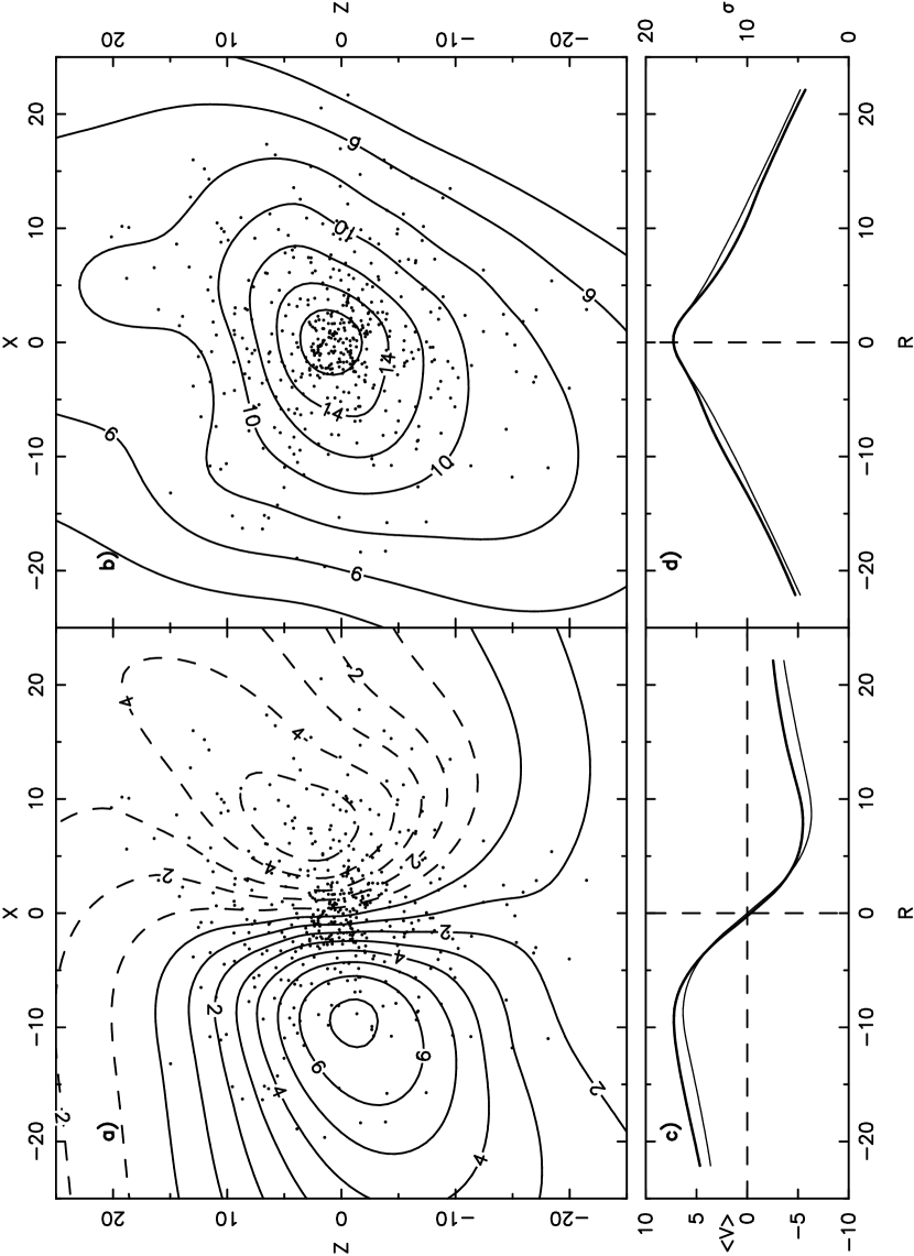
Figure 3:

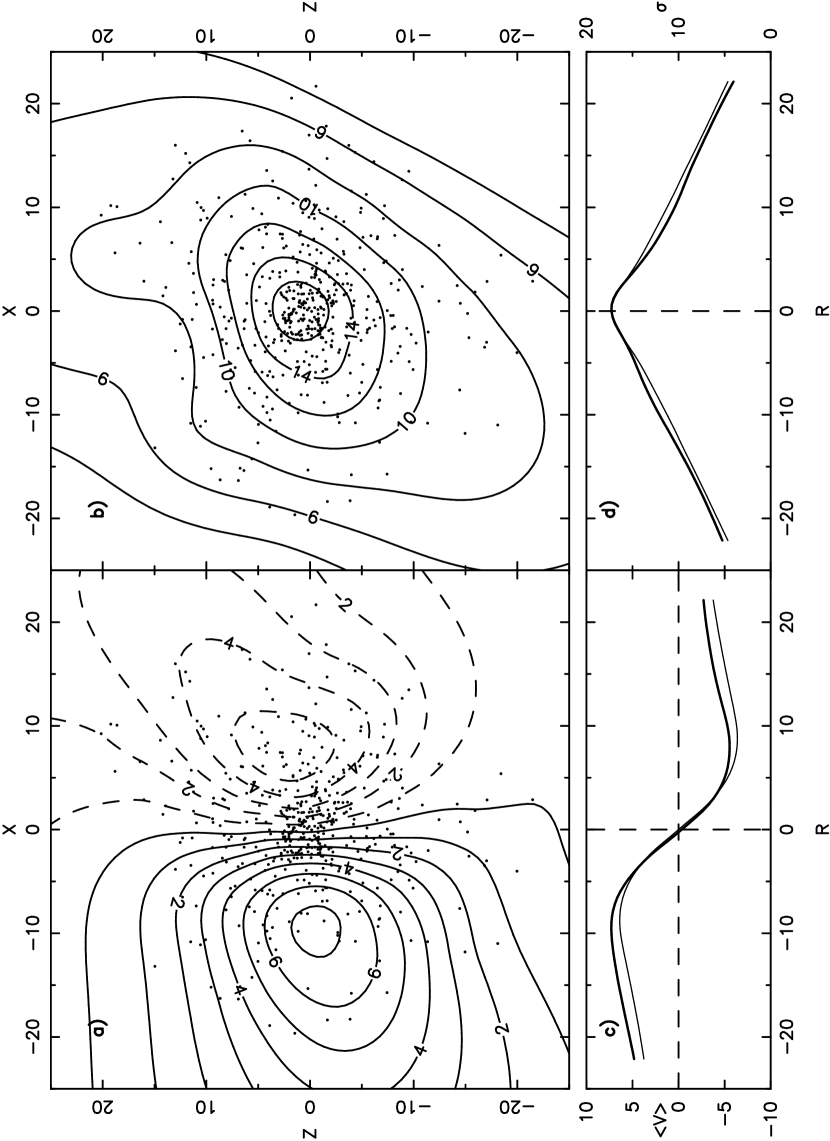
Figure 4:

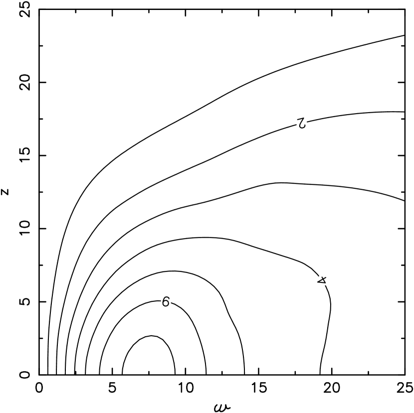
Figure 5:

Figure 6:

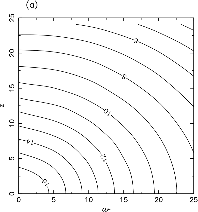
Figure 7:

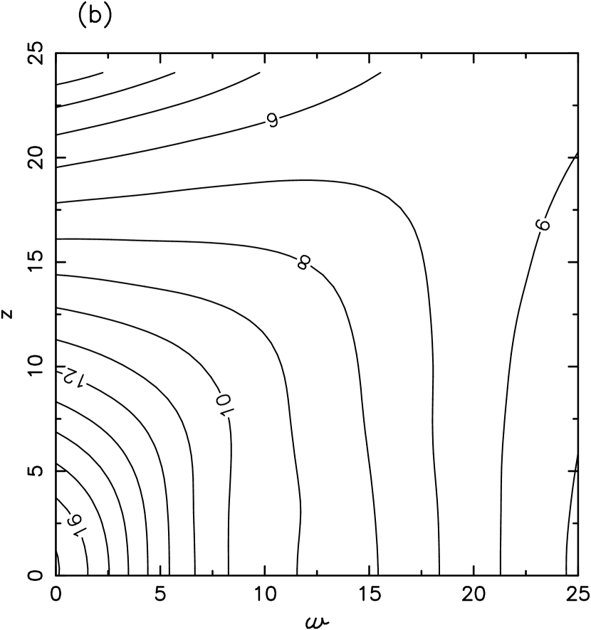
Figure 7:

Figure 8:

Figure 9:

Figure 10:

Figure 10:

Figure 11:

Figure 12:

Figure 12:

References

- Cudworth (1979) Cudworth, K. 1979, AJ, 84, 1312
- Cudworth (1994) Cudworth, K. 1994, private communication
- Cudworth & Monet (1979) Cudworth, K. M. & Monet, D. G. 1979, AJ, 84, 744
- Da Costa (1979) Da Costa, G. S. 1979, AJ, 84, 505
- Da Costa & Freeman (1976) Da Costa, G. S. & Freeman, K. C. 1976, ApJ, 206, 128
- Dejonghe & Merritt (1992) Dejonghe, H. & Merritt, D. 1992, ApJ, 391, 531
- Feast, Thackeray & Wesselink (1961) Feast, M. W., Thackeray, A. D. & Wesselink, A. J. 1961, MNRAS, 122, 433
- Gascoigne & Burr (1956) Gascoigne, S. C. B. & Burr, E. J. 1956, MNRAS, 116, 570
- Gebhardt et al. (1997) Gebhardt, K., Pryor, C., Williams, T. & Hesser, J. 1997, in preparation
- Gerhard (1993) Gerhard, O. E. 1993, MNRAS, 265, 213
- Gerhard & Binney (1996) Gerhard, O. E. & Binney, J. J. 1996, MNRAS, in press
- Geyer, Hopp & Nelles (1983) Geyer, E. H., Hopp, U. & Nelles, B. 1983, A&A, 125, 359
- Green & Silverman (1994) Green, P. J. & Silverman, B. W. 1994, Nonparametric Regression and Generalized Linear Models (Chapman & Hall, London)
- Gunn & Griffin (1979) Gunn, J. E. & Griffin, R. F. 1979, ApJ, 84, 752
- King (1966) King, I. R. 1966, AJ, 71, 64
- King (1981) King, I. R. 1981, QJRAS, 22, 227
- King et al. (1968) King, I. R., Hedemann, E., Hodge, S. M. & White, R. E. 1968, AJ, 73, 456
- Leonard & Merritt (1989) Leonard, P. J. T. & Merritt, D. 1989, ApJ, 339, 195
- Leonard, Richer & Fahlman (1992) Leonard, P. J. T., Richer, H. B. & Fahlman, G. G. 1992, AJ, 104, 2104
- Lupton, Gunn & Griffin (1987) Lupton, R., Gunn, J. E. & Griffin, R. F. 1987, AJ, 93, 1106
- Mayor (1985) Mayor, M. 1985, in IAU Colloq. 88, Stellar Radial Velocities, ed. A. G. Davis Philip, 35
- Mayor et al. (1997) Mayor, M., Udry, S., Meylan, G., Andersen, J., Nordström, B., Imbert, M., Maurice, E., Prévot, L., Ardeberg, A. & Lindgren, H. 1997, AJ, submitted (Paper I)
- Merrifield (1991) Merrifield, M. R. 1991, AJ, 102, 1335.
- (24) Merritt, D. 1993a, ApJ, 413, 79
- (25) Merritt, D. 1993b, in Structure, Dynamics and Chemical Evolution of Elliptical Galaxies, ed. I. J. Danziger, W. W. Zeilinger & K. Kjär (ESO: Munich), 275
- Merritt (1996) Merritt, D. 1996, AJ, 112, 1085
- Merritt (1997) Merritt, D. 1997, AJ, in press
- Merritt & Tremblay (1994) Merritt, D. & Tremblay, B. 1994, AJ, 108, 514
- Meylan (1987) Meylan, G. 1987, A&A, 184, 144
- Meylan & Mayor (1986) Meylan, G. & Mayor, M. 1986, A&A, 166, 122
- Meylan et al. (1995) Meylan, G., Mayor, M., Duquennoy, A. & Dubath, P. 1995, A&A, 303, 761
- Miller (1963) Miller, R. H. 1963, ApJ, 138, 849
- Müller (1988) Müller, H.-G. 1988, Nonparametric Regression Analysis of Longitudinal Data (Springer, Berlin)
- Murray, Jones & Candy (1965) Murray, C. A., Jones, D. H. P. & Candy, M. P. 1965, Royal Observatory Bulletins, 100, E81
- Peterson & King (1975) Peterson, C. J. & King, I. R. 1975, AJ, 80, 427
- Reijns et al. (1993) Reijns, R., Le Poole, R., de Zeeuw, T., Seitzer, P. & Freeman, K. 1992, ASP Conf. Ser. Vol. 50, Structure and Dynamics of Globular Clusters, ed. S. G. Djorgovski & G. Meylan, 79
- Roberts (1962) Roberts, P. H. 1962, ApJ, 136, 1108
- Rybicki (1986) Rybicki, G. B. 1986, in Structure and Dynamics of Elliptical Galaxies, IAU Sym. 127, ed. P. T. de Zeeuw (Kluwer: Dordrecht), 397
- Scott (1992) Scott, D. W. 1992, Multivariate Density Estimation (Wiley, New York)
- Thompson & Tapia (1990) Thompson, J. R. & Tapia, R. A. 1990, Nonparametric Function Estimation, Modeling, and Simulation (SIAM, Philadelphia), 102
- Wahba (1990) Wahba, G. 1990, Spline Models for Observational Data (SIAM, Philadelphia)
- Wahba & Wendelberger (1980) Wahba, G. & Wendelberger, J. 1980, Monthly Weather Review, 108, 1122
- White & Shawl (1987) White, R. E. & Shawl, S. J. 1987, ApJ, 317, 246