High Velocity Rain: The Terminal Velocity Model of Galactic Infall

Abstract

A model is proposed for determining the distances to falling interstellar clouds in the galactic halo by measuring the cloud velocity and column density and assuming a model for the vertical density distribution of the Galactic interstellar medium. It is shown that falling clouds with $N(H~{}I)~{}^{<}_{\sim}10^{19}~{}{\rm cm^{-2}}$ may be decelerated to a terminal velocity which increases with increasing height above the Galactic plane. This terminal velocity model correctly predicts the distance to high velocity cloud Complex M and several other interstellar structures of previously determined distance. It is demonstrated how interstellar absorption spectra alone may be used to predict the distances of the clouds producing the absorption.

If the distance, velocities, and column densities of enough interstellar clouds are known independently, the procedure can be reversed, and the terminal velocity model can be used to estimate the vertical density structure (both the mean density and the porosity) of the interstellar medium. Using the data of Danly and assuming a drag coefficient of $C_{D}\cong 1$, the derived density distribution is consistent with the expected density distribution of the warm ionized medium, characterized by Reynolds. There is also evidence that for $z~{}^{>}_{\sim}~{}0.4~{}{\rm kpc}$ one or more of the following occurs: (1) the neutral fraction of the cloud decreases to $\sim$ $31\pm 14\%$, (2) the density drops off faster than characterized by Reynolds, or (3) there is a systematic decrease in $C_{D}$ with increasing $z$. Current data do not place strong constraints on the porosity of the interstellar medium.

1 The “Hydrological Cycle” of the Interstellar Medium

“What goes up, must come down.” This is equally true for the interstellar medium of the Galaxy as for the Earth, assuming that the material in question does not have escape velocity. Due to the energy input in the midplane of the Galactic interstellar medium (ISM) from supernovae (SN) and stellar winds, we know that matter goes up (c.f, Spitzer 1990; McKee 1993). But how does it come down? In this paper, it is demonstrated that there is potentially important dynamical information contained in gaseous Galactic infall. Understanding the whole cycle is important since, barring merger events, the global density and pressure structure of the ISM is what determines the global star formation and is therefore important in understanding the evolution of the Galaxy.

First, what goes up? The mechanical energy input to the ISM is dominated by stellar winds and supernovae. In the 1970’s it was realized that if this energy were converted into thermal energy much of the volume of the ISM would be converted into hot, $T=10^{6}~{}K$ gas (Cox & Smith 1974; McKee & Ostriker 1977). Since this gas is buoyant and possibly overpressured, it will move away from the Galactic midplane (Shapiro & Field 1976; Norman & Ikeuchi 1989; McLow & McCray 1988 ). However, these flows are subject to several classes of instabilities (c.f., Field 1965; McLow & McCray 1988; Balbus 1988; Ferrara & Einaudi 1992) Therefore, it is reasonable that outflows, no matter how they occur in detail, are likely to form denser, colder lumps.

In the “galactic fountain” model, these lumps are identified with observed clouds of neutral hydrogen in the gaseous halo of the Galaxy, clouds which on average are moving with negative velocities toward the Galactic plane. Most notable in this regard are the so-called “High Velocity Clouds” (HVCs) with $|v|>70~{}{\rm km~{}s^{-1}}$. These clouds, first discovered by Muller, Oort, & Raimond (1963), have eluded all but one attempt to measure their distances (Danly, Albert, & Kuntz 1993), and are generally assumed to be located at greater than a few kiloparsecs. The origin of these clouds and their lower velocity companions is the subject of much debate and speculation (c.f., Ferrara & Field 1994, Wolfire et al. 1995). Regardless of their origin, one can ask the following question: given the existence of these neutral clouds, what are their dynamics? In particular, this paper address the observational puzzle raised by Danly (1989) whose ultraviolet absorption line study indicates that clouds appear to decelerate rather than accelerate as they approach the Galactic disk.

Previous works on this subject fall into two classes, which although illustrative, are incomplete in one important respect. The first class of models attempted to treat the global characteristics of this infall (Bregman 1980; Kaelble, de Boer, & Grewing 1985; Wakker 1990; Li & Ikeuchi 1992). Since the sizes of the falling clouds are significantly smaller than the Galaxy, the clouds were unresolved and it was assumed that the clouds fell ballistically. This assumption allowed cloud trajectories to be calculated for a large population of clouds, and the resulting distribution of velocities with respect to direction on the sky were calculated for comparison with the observational data. As will be shown, the ballistic approximation is likely to be inappropriate.

The second class of models calculates the full hydrodynamical evolution of individual clouds (Tenorio-Tagle et al. 1987; Comeron & Torra 1992; Lepine & Duvert 1994; Rand & Stone 1996). These models demonstrated how the impact of a high-velocity cloud of neutral hydrogen onto the H I disk could produce large-scale structures of H I and serve as a catalyst for star-formation. However, these models only considered high column density clouds, and neglected to take into account the fact that the Galaxy (or at least the local solar neighborhood) is now known to have an extended layer of ionized hydrogen, extending upward with a scale height of 1 kpc and comprising 25% of the total surface mass density of the interstellar gas (Reynolds 1993).

This paper discusses some simple considerations on the nature of Galactic infall and shows how the study of its dynamics has the potential to greatly improve our knowledge of the structure of the ISM. It is argued that drag forces on falling interstellar clouds are sufficient to lock many clouds to a terminal velocity which depends on the cloud height and column density. Measurement of a cloud velocity and column density may then be converted to $z$-height. Preliminary versions of this work have been presented as conference proceedings (Benjamin 1996a,b). In §2, the basic model is presented and it is argued that many clouds may be falling at a terminal velocity. §3 presents some potential applications of this concept to observational data. Finally §4 lists the principal results and implications of this work and notes the similarities between the proposed model and a more familiar but analagous process, namely the dynamics of terrestrial rain.

2 The Dynamics of Infall

Neutral hydrogen clouds above the Galactic plane must be surrounded by an external (ionized) gaseous medium, or they would disperse on a short timescale (Spitzer 1956). What is the effect of this gaseous medium on a cloud’s dynamics? Since neutral clouds are less buoyant than their surroundings, they will fall. For simplicity, it is assumed the cloud is restricted to move in the $z$ direction. Assuming a simple $v^{2}$ dependence for the drag force, the equation of motion is

$$m_{c}\frac{dv_{c}}{dt}=\frac{1}{2}C_{D}\rho_{h}(z)[v_{c}-v_{h}(z)]^{2}A_{c}-m_{c}g(z)~{}.$$ (1)

The mass, surface area, and velocity of the cloud are $m_{c}$, $A_{c}$, and $v_{c}$; the halo gas density, velocity, and gravitational acceleration at height $z$ above the Galactic plane are $\rho_{h}(z)$, $v_{h}(z)$, and $g(z)$. The drag coefficient, $C_{D}$, indicates the efficiency of momentum transfer to the cloud, the accompanying factor of $1/2$ is conventionally (but unfortunately not always) included. The first term in the right hand side represents the decelerating force of ram pressure; the second is the accelerating force of gravity. If these two forces are in balance, $dv/dt=0$ and the cloud has reached “terminal velocity”, $v_{T}$. Ballistic calculations mentioned in the previous section ignored the deceleration term. Hydrodynamical calculation of high velocity clouds hitting the disk underestimated the deceleration by underestimating $\rho_{h}(z)$ or used a high $m_{c}/A_{c}$.

It is assumed here that (1) the cloud can maintain itself as a discrete entity, and (2) the above equation provides a first approximation to its motion. The first point is at issue because before the cloud approaches terminal velocity it is subject to Rayleigh-Taylor instabilities, and it is always subject to Kelvin-Helmholtz instabilities. Recent numerical simulations (MacLow et al. 1994; Jones, Ryu, & Tregillis 1997) have demonstrated how inclusion of even weak magnetic fields may inhibit these instabilities. The second point is at issue because although it clear that the drag force must increase with velocity, it is not known what functional form will best characterize the drag. Equation (1) assumes that is the pressure difference from the front to back of the cloud, i.e. the ram pressure, which is responsible for the deceleration. The retarding force is thus proportional to $v^{2}$ with constant of proportionality $C_{D}$. In actuality, the process of deceleration is probably more complicated and depends upon the viscosity of the ISM, the deformation of the cloud, and the flow pattern around the cloud. This issue is best resolved through numerical simulations. The most recent simulations of Jones et al (1997) indicate that the global deceleration of a cloud is proportional to $v^{2}$, and $C_{D}\cong 1$, although it was necessary to modify this drag coefficient to take into accout the lateral expansion of the cloud and the presence of magnetic fields.

2.1 The Terms and Their Uncertainties

We now discuss each of the terms in equation (1), the values used for this paper and their uncertainties:

$g(z)$: The gravitational acceleration is taken from Wolfire et al. (1995) and Spergel (1994). This is shown in Figure 1, and can be fit to within 15% by $g(z)=9.5\times 10^{-9}\tanh(z/400~{}pc)$. At some large height, the assumption of purely vertical trajectory will break down, the value of this depends on the initial conditions for the cloud, e.g., whether it starts out initially co-rotating with the disk below, etc.

$m_{c}$: The mass of the cloud may either increase or decrease over time. Which occurs and to what degree depends upon the particular environmental conditions and assumed input physics. The cloud can gain mass by “sweeping up” either ambient halo gas or other slower moving clouds as it falls. On the other hand, Kelvin-Helmholtz and possibly Rayleigh-Taylor instabilities will act to strip the cloud of mass and could potentially disrupt the cloud entirely (Klein, McKee, & Colella 1994; Jones, Kang, & Tregillis 1994). Inclusion of modest magnetic fields will ameliorate this effect (MacLow et al. 1994; Jones, Ryu, & Tregillis 1997). Without detailed simulations, it is hard to know what the net effect is on the cloud mass and motion. Here a constant mass is assumed.

$A_{c}$: It is assumed that the cloud is flattened in the direction of motion. The cloud mass is $m_{c}=\mu A_{c}\int n_{c}(z)~{}dz=\mu A_{c}N_{c}$, where $n_{c}(z)$ is the cloud particle density, $N_{c}$ is the column density, and $\mu$ is the mean mass per particle. The surface area term in the equation of motion may then be divided out. The geometry of the cloud, i.e. whether it is rod-like (high $m_{c}/A_{c}$) or sheet-like (low $m_{c}/A_{c}$), will affect the amount of drag. By making this assumption, the effects of the geometry, and the associated uncertainties, have been subsumed into the drag coefficient, $C_{D}$.

$C_{D}$: The uncertainty in this coefficient will need to be addressed by numerical simulations. For a perfectly streamlined cloud, $C_{D}=0$; for perfect momentum transfer, $C_{D}=2$. $C_{D}$ can exceed 2 if the flow pattern yields an underpressurized region behind the cloud. This work uses $C_{D}=1$ as a starting guess (Jones, Ryu, & Tregillis 1997). But $C_{D}$ may depend on several factors: the mass and velocity of the cloud, the halo density and temperature, the relative importance of magnetic fields, radiative cooling, etc. And it may depend upon the history of the cloud, i.e. the drag coefficient will change over time as the cloud deforms and tries to adjust to its motion through the background. Comparison of indvidual cloud morphologies (Odenwald 1988; Wakker & Schwarz 1991) to simulations of cloud-halo interactions will provide independent constraints on the relevant input physics and the proper value of the $C_{D}$.

$n_{h}(z)$: The density structure of the gaseous halo is the great unknown. If the halo were uniform, isothermal, static, and dominated by thermal pressure, a simple application of the equation of hydrostatic equilibrium would yield the density structure (Spitzer 1956; Wolfire et al. 1995). However, this situation is far from being the case, with nonthermal pressure being more important than thermal pressure sources at least up to a few ${\rm kpc}$ (Boulares & Cox 1990). With many of the theoretical issues relating to the density structure of the interstellar medium still outstanding, it is probably far safer to stick to using the observationally determined density structure. Three different density distributions are considered and shown in Figure 1:

(A) The mean density of the warm ionized layer of H II using the parameterization of Reynolds (1993): $n_{h}(z)=0.025~{}e^{-z/910~{}pc}~{}cm^{-3}$.

(B) The “Reynold’s layer” plus the mean H I density of Dickey & Lockman (1990), which consists of three components: two Gaussians of central densities $0.395$ and $0.107~{}cm^{-3}$ and FWHM of $212$ and $530~{}pc$, and an exponential with central density $0.064~{}cm^{-3}$ and scale height of $403~{}pc$.

(C) The above two plus an isothermal “hot” halo with $T=10^{6}~{}K$ as prescribed by Wolfire et al. (1995), $n_{h}(z)=1.1\times 10^{-3}(1+(z_{{\rm kpc}}^{2}/19.6))^{-1.35}~{}cm^{-3}$.

The third component, unlike the first two is not an observationally derived quantity, but is constructed by assuming the presence of a hydrostatic isothermal $T=10^{6}~{}K$, halo, and determining the midplane density by matching the X-ray emission data of Garmire et al. (1992). The only independent information on the halo gas density above $\sim 3~{}{\rm kpc}$ is by studying neutral cloud morphologies and dynamics. For instance, the diffuse $H\alpha$ observations of a neutral Magellanic Stream cloud by Weiner & Williams (1996) together with assumptions on the nature of the cloud-halo interaction indicate a gas density for the halo of $n_{h}=10^{-4}~{}cm^{-3}$ at $z>>10~{}{\rm kpc}$.

$v_{h}(z)$: It is assumed that the velocity of the background medium is static with respect to the Local Standard of Rest. This assumption may break down close to the Galactic plane, where SN and stellar wind driven turbulence drive large scale mass motions. It must also break down well above the plane, since it is not possible that the halo corotates with the disk up to infinity. At some height, the halo must lag behind the disk. This tendency is possibly observed by Rand (1997), whose observations of NGC 891 indicate that at a height of $5~{}{\rm kpc}$, the $H\alpha$ rotation curve lags rotation in the plane by approximately $15~{}{\rm km~{}s^{-1}}$.

2.2 The Terminal Velocity Model

In the simplest of all possible galaxies, interstellar clouds would all be falling at their terminal speed,

$$|v_{T}(z)|=\sqrt{\frac{2g(z)N_{H~{}I}}{C_{D}f_{c}n_{h}(z)}}~{},$$ (2)

where the cloud neutral fraction is $f_{c}=N_{H~{}I}/(N_{H~{}I}+N_{H~{}II})$. This factor is introduced since what matters in cloud dynamics is the total column density but observational techniques generally only allow measurment of the neutral column density. In fiducial units, and using the analytical formulation for the density structure of the Reynold’s layer, this is

$$|v_{T}(z)|=26~{}{\rm km~{}s^{-1}}(C_{D}f_{c})^{-1/2}\left(\frac{N_{H~{}I}}{10^{19}~{}cm^{-2}}\right)^{1/2}\left(\frac{g(z)}{g(1~{}{\rm kpc})}\right)^{1/2}\left(\frac{n_{h,o}}{0.025~{}cm^{-3}}\right)^{-1/2}e^{z/2H}$$ (3)

.

Since typical halo cloud speeds are similar to the value of $|v_{T}|$, the effects of drag can not be automatically dismissed. The appendix shows the typical time and distances necessary for a cloud with constant gravitational acceleration to converge to terminal velocity in both a uniform and a porous interstellar medium. Since halo density and gravitational acceleration change as a function of position, the terminal speed is position dependent. $|v_{T}(z)|$ is defined as the local terminal speed; this is plotted for clouds of varying column density and different halo density structures in Figure 2.

Do clouds reach a terminal speed? To answer this question, equation (1) is used to calculate the trajectories of clouds with $N_{H~{}I}=10^{18}~{}{\rm cm^{-2}}$ , $10^{19}~{}{\rm cm^{-2}}$ , and $10^{20}~{}{\rm cm^{-2}}$ dropped at rest from heights of $z_{i}=1,5,~{}{\rm and}~{}8~{}{\rm kpc}$. The trajectories, together with the ballistic trajectories and the local terminal velocity curves, are shown in Figure 3 for density structure of the warm ionized medium only. The points note the location after $n$ ($n=1,2,..$) free-fall times, $t_{ff}=\sqrt{2z_{i}/g(z_{i})}$. The highest velocity that can be achieved by a falling cloud is the escape velocity, $v_{esc}\approx 500~{}{\rm km~{}s^{-1}}$ (Binney & Tremaine 1987).

For clouds of column density $N(H~{}I)=10^{20}~{}{\rm cm^{-2}}$, the cloud is significantly decelerated from a ballistic trajectory, but its velocity never closely resembles the terminal velocity. On the other hand, these clouds are relatively rare. For reference, the total H I column density through the H I disk is $6\times 10^{20}~{}{\rm cm^{-2}}$ (Dickey & Lockman 1990). Clouds with $N(H~{}I)=10^{19}~{}{\rm cm^{-2}}$ are much more significantly decelerated, and within 1 kpc of the disk, their velocities tend to be within 50% of the local terminal velocity. Most usefully, clouds with $N(H~{}I)=10^{18}~{}{\rm cm^{-2}}$ will rapidly lock on to the local terminal velocity. These clouds spend a proportionally longer period of their lifetime at or near terminal velocity rather than in the ballistic phase. The rest of this paper will use the shorthand description “low”, “medium” and “high” column density for clouds of $N(H~{}I)=10^{18}~{}{\rm cm^{-2}},10^{19}~{}{\rm cm^{-2}},~{}{\rm and}~{}10^{20}~{}{\rm cm^{-2}}$, respectively.

These calculations indicate that the assumption of terminal velocity is reasonable starting point for predicting the cloud velocities for clouds with $N(HI)~{}^{<}_{\sim}10^{19}~{}{\rm cm^{-2}}$, with increasing accuracy for decreasing cloud column density.

3 The Terminal Velocity Model: Tests and Applications

The terminal velocity model allows a distance prediction for every interstellar cloud with a negative vertical velocity and measured column density. Although the range of applicability of the model must ultimately be tested by observational studies, it is clear that there exist certain fundamental limits on this method. First, given the existence of postive velocity clouds, it is clear that equation (1) must be modified to include additional sources of momentum. It is reasonable to assume that the same momentum sources will also affect some subset of downward travelling clouds. Second, as shown above, clouds will have some sort of dynamical history, and this history may affect the space velocity. At one extreme, the space motion of a high column density cloud in low density enviroments, such as a cloud in the Magellanic Stream, will largely retain a “dynamical memory” of its origin. At the other extreme, a cloud which forms in situ in the halo may slowly grow in column density, always adjusting its velocity to match the local terminal velocity, thus retaining no “memory” of its previous motion.

There are three primary ways in which this model may be applied to observations:

1) Assume $C_{D}$ and $n_{h}(z)$. Measurement of $N_{H~{}I}$ and $v$ allows determination of the distance, $z$.

2) Assume $C_{D}$. Measurement of $N_{H~{}I}$, $v$, and $z$ allows determination of the density structure of the halo, $n_{h}(z)$.

3) Assume $n_{h}(z)$. Measurement of $N_{H~{}I}$, $v$, and $z$ allows an empircal calculation of the drag coefficient, $C_{D}$.

It seems likely that the first application will be the most useful, § 3.1 shows how the model may be invaluable for interpreting UV and optical absorption line data. The second application in § 3.2 will require a large and systematic effort of UV and optical absorption line studies to independently obtain cloud distances, and could provide an invaluable probe for the mean density and porosity of the interstellar medium. The third application, also discussed in § 3.2 will probably only become necessary if theoretical considerations are not able to sufficiently limit the range of variation of $C_{D}$.

3.1 How to Predict Cloud Distances

3.1.1 Tests

Figure 4 shows negative velocity clouds with $|b|>30$ and $|z|^{>}_{\sim}200~{}pc$ for which distance limits have been obtained. Data are taken from Kuntz and Danly (1996), Danly et al. (1992), Albert et al (1993), de Boer et al. (1994), Benjamin et al. (1996), Wesselius & Fejes (1973), and Benjamin, Hiltgen, & Sneden (1997). Also included is a line indicating the negative velocity extent of UV absorption as a function of star height from Danly (1989). This last study was able to put onto a more quantitative footing the already empirically recognized fact that the higher the cloud velocity, the more distant it is likely to be (c.f., Welsh, Craig, & Roberts 1996; de Boer et al. 1994). This figure shows, despite a paucity of accurate distances, a trend of velocity increasing with $z$. Here, the model is compared against clouds of known distance, namely Complex M (Danly, Albert, & Kuntz 1993), the “IV Arch”(Kuntz & Danly 1996), the Ursa Major IVC (Benjamin et al. 1996), and several clouds observed by Albert et al (1993). The clouds chosen have $|b|>50$, in order to minimize the effects of galactic rotation, and the values of velocity and column density used in equation (2) are corrected for projection effects assuming $v_{z}=v|csc~{}b|$ and $N_{z}=N_{H~{}I}|sin~{}b|$. The observed cloud parameters and their references are shown in Table 1, along with a comparison between the distance predictions and the observed distance limits. In all cases, it is assumed that $C_{D}=1$ and $f_{c}=1$, except for the IV Arch, where independent information indicates that $f_{c}\cong 0.44$ (see discussion in the next section). Predictions are shown for density models A and B.

Allowing for uncertainties in the stellar distances (typically $25\%$), the model successfully predicts the distances for eight of ten clouds, including the HVC Complex M, assuming the warm ionized medium is principally responsible for their deceleration. For clouds at sufficiently high $z$, these distances predictions probably tend to be overestimates since the ambient pressure is lower, and the expected neutral fraction of clouds is expected to be $f_{c}<1$ (Songaila, Cowie, & Weaver 1988; Ferrara & Field 1994). Accounting for this will have the effect of reducing the predicted distance by $\Delta z\cong H\ln(f_{c}^{-1})$, where $H=910~{}pc$ for the warm ionized density distribution.

The case of the Ursa Major cloud deserves special comment. The model correctly predicts this distance to this high column density molecular cloud, assuming that both the H I and H II layer contribute to its deceleration. Since this cloud has sufficiently high column density that it should be travelling faster than much of the H I that makes up the high latitude H I layer, it is not surprising that it should feel the decelerating force of the H I layer. Since the other H I clouds are presumably also falling, the ram pressure due to the H I layer will be reduced because the relative velocity of the high column density cloud of interest and the “typical” H I cloud. If $R=N_{c}/N_{l}$ is the ratio of the column density of the heavy cloud to the column density of the “typical” cloud making up the H I layer, and $n_{H~{}I}$ and $n_{H~{}II}$ are the mean densities of the H I and H II layer, then the terminal velocity of the heavy cloud, $v_{c}$ is

$$v_{c}=v_{l}\left[\frac{n_{H~{}I}+\sqrt{Rn_{H~{}II}^{2}+(R-1)n_{H~{}I}n_{H~{}II}}}{n_{H~{}I}+n_{H~{}II}}\right]$$ (4)

where $v_{l}=\sqrt{2N_{l}g/(C_{D}n_{H~{}II})}$ is the terminal velocity of the “typical” H I layer cloud in the H II layer. Solving for the velocity difference between the cloud and H I layer that allows a match between the terminal velocity model and the observed distance yields $v_{l}=23~{}{\rm km~{}s^{-1}}$, which corresponds to a cloud column density of $N_{l}=10^{18.9}~{}{\rm cm^{-2}}$.

3.1.2 Predictions

The line of sight toward HD 93521 ($z=1.5\pm 0.4~{}{\rm kpc}$, $b=62.2$) is one of the best studied halo lines of sight, and contains an unusually large number of absorption components. It therefore provides a good test case for predicting cloud distances. Here, the terminal velocity model is used to predict the distances to the clouds observed in UV absorption line data of Spitzer & Fitzpatrick (1993). The measured velocities, column densities, and predicted distances are in Table 2. The $N(H~{}I)$ column density is estimated by taking advantage of the fact that S II is a very good tracer for H I, i.e. the ratio N(S II)/N(H I) is relatively constant, $N(H~{}I)_{s}=10^{4.76}N(S~{}II)$ (c.f., Spitzer & Fitzpatrick 1993). The advantage of this assumption is that a single self-contained measurement may be used to determine cloud distance; both the cloud column density and velocity may be obtained from a single spectrum. Other ions (including the optically detectable ${\rm Ca^{+}}$ or ${\rm Ti^{+}}$) could also be used provided a similar “correction factor”, which allows conversion of $N_{ion}$ to $N(H~{}I)$. For many ions, however, it has been demonstrated that this “correction factor” (which depends on depletion and ionization effects) is velocity dependent, so care must be taken (c.f., Jenkins 1987).

The cloud neutral fraction, $f_{c}$, is determined by comparison of the ratio of column densities of two ions to photoionization models of the cloud. For the data of Spitzer & Fitzpatrick (1993) the ratio $N(S~{}III)/N(S~{}II)$ is used. Theoretical values for this ratio are calculated using version 84.12a of the photoionization code CLOUDY (Ferland 1993) to model the cloud as a plane-parallel, constant density slab photoionized by the predominantly stellar ionizing spectrum of Bregman & Harrington (1986) or the X-ray emission spectrum of Benjamin & Shapiro (1996). (Note that given the cloud’s deceleration, the constant density assumption is unlikely to be valid. The effect of a non-uniform density on the ionization structure is deferred to future work.) For $-4.5<\Gamma<-2$ and stopping H I column densities $18<logN(H~{}I)_{end}<19.5$, the column density ratio is well fit to within 20% by

$$\log{\frac{N(S~{}III)}{N(S~{}II)}}=0.9\log\Gamma+B-0.25N~{},$$ (5)

where $N=logN(H~{}I)_{end}-18$ and $B=2.90$ for the Bregman & Harrington spectrum and $B=3.25$ for the Benjamin & Shapiro spectrum. For the Bregman & Harrington ionizing spectrum, the ionization parameter required to match the observed values lies in the range $\log~{}\Gamma=-4.25$ to $-3.60$. $f_{c}$ can be estimated by balancing the ionizing photon flux, $\phi$ (H ionizing photons $s^{-1}$ ${\rm cm^{-2}}$), with the total number of recombinations in some column of length, $l$, so that $\phi\cong n_{H}^{2}\alpha l$, where $\alpha\cong 3\times 10^{-13}{\rm cm^{3}}~{}s^{-1}$ is the recombination coefficient. Since the ionization parameter is $\Gamma=\phi/(cn_{H})$, $N(H~{}II)=\Gamma c/\alpha$, and therefore $f_{c}=N_{H~{}I}/(N_{H~{}I}+(c\Gamma/\alpha))$. The resultant values of $f_{c}$ are in Table 2. Use of the X-ray ionizing spectrum of Benjamin & Shapiro (1996) would increase $f_{c}$ by $\sim 0.2$.

One test of the accuracy of the predictions is that the derived cloud distances must not exceed the distance of the star. Within the estimated uncertainties, they satisfy this criterion, with the exception of component 5, which is a marginal detection. High resolution optical spectroscopy of suitable target stars in the vicinity of HD 93521 could be used to test these predictions. Albert (1983) has already reported observations for 32 LMi ($z=150~{}pc$) a star separated from HD 95321 by $3.8^{\circ}$. She detects no absorption at any velocity. This nondetection is consistent with all the distance predictions, with the possible exception of component 7 at $v=-10.2~{}{\rm km~{}s^{-1}}$. However, for the lowest velocity components, small errors in measurement of the velocity can lead to large errors in the derived distance. This fact combined with the likelihood that additional momentum sources will be important close to the galactic plane means this method may not be a reliable way to determine cloud distances below $\sim 200~{}pc$. Nevertheless, this type of analysis can be repeated wherever one has UV and optical absorption line data and holds the promise of significantly improving our knowledge of the structure of the interstellar medium.

3.2 How to Determine the Density Structure of the Halo

If there existed a large population of interstellar clouds with known distances, velocities, column densities, and neutral fractions, the procedure described above could be inverted, and one could use these clouds plus the terminal velocity model to constrain the mean density structure of the gaseous halo, the porosity, and the variation with galactic longitude. As Figure 4 indicates, the number of cloud for which tight distance brackets have been obtained is regretably small. However, one can use the UV absorption study of Danly (1989) to address this question, assuming that the distance to the star is approximately the distance to the cloud producing the most negative velocity absorption. This assumption is more likely to be true in the North Galactic Hemisphere, which appears to be full of infall at a large range of $z$ and $v$ (Danly 1989; Kuntz & Danly 1996) than in the South Galactic Hemisphere, which has less infalling gas.

3.2.1 The Mean Density of the Gaseous Halo

Rearranging the terms in equation (2), the mean density of the halo as a function of $z$ as derived by cloud kinematics is

$$C_{D}f_{c}n^{kin}_{h}(z)=\frac{2N_{H~{}I}g(z)}{v^{2}}$$ (6)

By measuring the column density and velocity of cloud and estimating the gravitational acceleration at the location of the cloud, one can solve for the local ambient density at the location of the cloud, short of uncertainties in the appropriate value of the drag coefficient and ionization fraction. Table 3 lists some of the target stars of Danly (1989), their height above the Galactic plane, $z_{star}$ (which is assumed to equal to $z_{cloud}$), the most negative velocity of absorption, $v_{-}$. The sample has been limited to lines of sight with $|b|>50$ in order to avoid uncertainties associated with galactic rotation and projection effects, and $N(H~{}I)>10^{17.9}~{}{\rm cm^{-2}}$ where the column densities become highly uncertain. For the cases of BD +38 2182 and HD 93521, the data have been updated to be consistent with those in Table 1. The column density $N(H~{}I)$ in the velocity range $v_{-}\pm 5~{}{\rm km~{}s^{-1}}$ density is obtained either by integrating the H I profiles (Danly et al 1992) in the direction of each star or, when no profiles were available, by locating the stars on the H I emission maps of Kuntz & Danly (1996). Uncertainties were not calculated for the derived density, since they were not available for all input parameters.

For each line of sight, the kinetically derived gas density times $C_{D}f_{c}$ is tabulated. The derived density at low $z$ ($z<100~{}pc$) is in good agreement with the midplane density of the warm ionized medium (Weisberg, Rankin, & Boriakoff 1987) although it arises from an independent line of reasoning. Given the expectation that the model should break down at low $z$ due to additional momentum sources and that the clouds producing this absorption lie within the expected confines of the Local Hot Bubble (Cox & Reynolds 1987), this agreement may merely be fortuitous.

For the more distant stars (and presumably more distant clouds) the derived density decreases as a function of $z$, in agreement with expectations. However, the derived density drops off faster than one would expect in the density models considered. This is shown in Table 3, where the ratio of the derived kinematic density to the expected density, $n^{kin}(z)/n_{h}(z)=C_{D}f_{c}$ is tabulated. Figure 5 illustrates this graphically for the warm ionized medium density. For clouds (stars) below 400 pc, $C_{D}f_{c}=0.92\pm 0.09$, where the line of sight towards HD 219688 has been excluded as anomalous, and the uncertainty is the standard deviation of the derived values and does not reflect measurement errors in the input parameters. For stars between 500 pc and and 3300 pc, $C_{D}f_{c}$ decreases to $0.31\pm 0.14$. The data do not allow one to characterize whether there is smooth or abrupt decrease. Above 3300 pc, $C_{D}f_{c}$ increases to values significantly greater than one.

If $C_{D}\cong 1$, one explanation for this trend is that the cloud neutral fractions decline to $f_{c}\approx 0.3$ for $|z|~{}^{>}_{\sim}~{}400~{}{\rm pc}$. This trend is consistent with theoretical expectations (Ferrara & Field 1994), and the value is consistent with the derived neutral fractions obtained by comparison of column densities of S II and S III with photoionization model as described in the previous section. Other possible explanation are a systematic decrease of $C_{D}$ at high $z$, or the mean density droping somewhat faster the exponential model used by Reynolds(1993). Differentiating among these possibilities will require a more thorough observational investigation, plus a better theoretical characterization of how $f_{c}$ and $C_{D}$ might vary with height.

It is important to remember that equation (2) yields the halo density at the location of the cloud, but the $z$ reported is that of the star in which absorption is detected. Therefore the reported value of $n^{kin}(z)$ will be an upper limit on the gas density at $z_{star}$, since the gas density will decrease between $z_{cloud}$ and $z_{star}$. Thus if clouds are confined to a layer with $z_{max}$, $C_{D}f_{c}$ will be larger than its true value if $z_{star}\geq z_{max}$. This provides a viable explanation for the large increase in $C_{D}f_{c}$ for $|z|>3300~{}pc$.

3.2.2 The Porosity of the Halo

Once the effect of column densities is factored out, assuming a model for the mean density of the gaseous halo defines a position-velocity curve. If one assumes that regions of hot, $T\cong 10^{6}~{}K$ gas in the halo are in pressure equilibrium with the warm, $T=10^{4}~{}K$ ionized gas, the density in the hot patches will be $\sim 100$ times lower. Every time a cloud hits one of these patches, it will start to accelerate, introducing scatter and widening the position-velocity curve into a band. This provides an upper limit on the porosity, since observational error, uncertain projection effects, and Galactic rotation will introduce their own scatter into the velocity-distance relationship.

Unfortunately at the current time, the data barely define a good mean value, let alone a scatter. In the appendix, it is shown how the velocity range, $\Delta v$ depends on the linear filling fraction, $f$, and “cell length”, $L$, for ISM with constant mean density. The following is an example of how this may be used to estimate the effect of patchiness on cloud dynamics: Assume that the velocity scatter in the terminal velocity relationship for clouds of column density $N(H~{}I)=10^{18}~{}{\rm cm^{-2}}$ is found to be $\Delta v=10~{}{\rm km~{}s^{-1}}$ at all $z$. Convert $\Delta v$ to $\Delta\tilde{v}(z)$ by dividing by the terminal velocity shown in Figure 2. These values can be converted to a loci of filling factor and cell length using Figure A1. Assuming a filling factor sets the normalized cell length, which can be converted to a physical length by multiplying by the convergence length $z_{T}=v_{T}(z)^{2}/g(z)$. If $f=0.8$, to introduce scatter greater than $\Delta v=10~{}{\rm km~{}s^{-1}}$ would take cell lengths of greater than $L_{cell}\sim~{}1~{}{\rm kpc}$, much larger than the scales over which the terminal velocity will change. However, if $f=0.2$, then cell lengths must only be greater than $L_{cell}\sim 200~{}pc$, a value low enough to be of some interest. Since, in general, the cell lengths are sufficiently large that they approach the scale on which the mean density and gravitational acceleration are changing, a better method to estimate of the scatter around the terminal velocity curve would be to perform Monte Carlo simulations of clouds falling through different assumed density distributions. This is deferred to later work.

It is important to note that the pattern of cloud velocity increasing with height observed by Danly (1989) already indicates that the density of the halo ISM is at some level homogeneous, at least on the scales probed by galactic infall, unless one argues that that the observed correlation is a chance occurence or there is some alternative explanation. Danly’s results set an upper limit on the amount of scatter in the position-velocity curve. This corresponds to $\Delta v~{}^{<}_{\sim}30~{}{\rm km~{}s^{-1}}$. Unfortunately, cell sizes necessary to produce such scatter are sufficiently large ($z>1~{}{\rm kpc}$) as not to provide any interesting limits on the porosity of the interstellar medium.

4 High velocity rain

There is a time-honored connection between the study of neutral halo clouds and understanding of the gaseous halo of the Galaxy. The existence of these clouds discovered by Munch & Zirin (1961) prompted Spitzer (1956) to infer the existence of a large gaseous extent for the Galaxy. Here, studies on the dynamics of the same clouds by Danly (1989) and also by Albert (1983), have prompted this work which is an attempt to characterize the structure of the ambient interstellar gas at high $z$. The density structure derived from cloud kinematical arguments, it is argued, is similar to the density of the warm ionized medium as determined by pulsar dispersion measures, and shows evidence for a decrease in cloud neutral fractions with increasing $|z|$.

The critical factor that differentiates this work from previous characterizations of galactic infall is the identification of the recently discovered extent of the warm ionized medium (Reynolds 1989) as occupying the intercloud regions. The warm ionized medium, comprising 25% of the total surface mass density of the interstellar medium, must have an important effect on the trajectories of neutral clouds. Instead of treating the cloud motions as ballistic in a low density, dragless intercloud medium (c.f., Oort 1954, Field & Saslaw 1965, McKee & Ostriker 1977), the terminal velocity model represents the opposite extreme. Instead of no drag forces, cloud motions are governed entirely by drag forces. Instead of cloud motions being essentially random, they are systematic. Since the motions are systematic, their distances can be predicted and tested. The model correctly predicts the distances of eight of ten interstellar clouds for which data were available.

In characterizing the dynamics of Galactic infall, Danly (1989) referred to falling clouds of low column density as “drizzle” and clouds of high column density as “storms”. The terminal velocity model suggests that this analogy extends to the dynamical level. Much of the physics discussed here applies equally well to the dynamics of raindrops as to falling interstellar clouds (c.f. Foote & du Toit 1969). In both cases, there is a phase change, a loss of buoyancy, and an acceleration up to a terminal velocity in a (presumably) exponential density structure. There are also important differences, most notably that liquid water unlike neutral hydrogen clouds is incompressible. Nevertheless, this has been a useful analogy in developing this work, and questions that arise in comparing the two systems may provide interesting avenues for future exploration.

Appendix A Convergence to Terminal Velocity in a Uniform and Porous Medium

In a uniform density medium with constant gravitational acceleration, a falling cloud will ultimately reach a terminal velocity. It is convenient therefore to have a formulation that indicates how quickly a cloud approaches terminal velocity, a value that can be compared with how quickly the local terminal velocity changes.

Consider the case of a cloud in a uniform density gas with constant $C_{D}$ and $g$, writing equation (1) in dimensionless form where $\tilde{v}=v/v_{T}$, $\tilde{t}=t/t_{T}$, and $\tilde{z}=z/z_{T}$, where $v_{T}$ is a positive definite quantity, and negative velocities indicate motion toward the Galactic plane. The “convergence time”, $t_{T}=v_{T}/g$, and “convergence length”, $z_{T}=v_{T}^{2}/g$ are the typical time and length scales for a cloud to approach the terminal velocity. The equation of motion is

$$\frac{d\tilde{v}}{d\tilde{t}}=\tilde{v}^{2}-1~{}.$$ (A1)

Leaving aside the case of cloud initially moving away from the Galactic plane (in which case gravitational deceleration and drag have the same sign), the solution for equation (A1) breaks into the case in which the cloud is accelerating to the terminal speed from below ($0>\tilde{v}_{o}>-1$) and the case in which the cloud is decelerating to the terminal speed ($-1>\tilde{v}_{o}>-\infty$).

Solving equation (A1) for the velocity as a function of time yields

$$\tilde{v}=\frac{\kappa\pm e^{2\tilde{t}}}{\kappa\mp e^{2\tilde{t}}}~{},$$ (A2)

where

$$\kappa=\pm\frac{\tilde{v}_{o}+1}{\tilde{v}_{o}-1}~{},$$ (A3)

where the upper sign is for the decelerating case, and the lower is for the accelerating case. The position as a function of time is

$$\tilde{z}-\tilde{z_{o}}=\ln(\frac{\kappa\mp 1}{\kappa\mp e^{2\tilde{t}}})+\tilde{t}~{}.$$ (A4)

The relationship between position and velocity for both cases is

$$\tilde{z}-\tilde{z_{o}}=\frac{1}{2}\ln\left[\frac{\tilde{v}^{2}-1}{\tilde{v}_{o}^{2}-1}\right]~{}.$$ (A5)

How quickly does the cloud approches its terminal speed? The time at which the cloud has reached a velocity midway between its original velocity and the terminal velocity is $\tilde{v_{1/2}}=(\tilde{v_{o}}-1)/2$. For both the accelerating and decelerating cases this is

$$\tilde{t}_{1/2}=\frac{1}{2}\ln(\frac{\tilde{v_{o}}-3}{\tilde{v_{o}}-1})=c_{t}~{}.$$ (A6)

For $v_{o}$ between 0 and -2, $c_{t}$ ranges from 0.55 to 0.25. This corresponds to a distance travelled of

$$\tilde{z}_{1/2}=\ln(\frac{1}{2}\sqrt{\frac{\tilde{v_{o}}-3}{\tilde{v_{o}}-1}})=c_{z}~{},$$ (A7)

where $c_{z}$ ranges from 0.14 to 0.43 for $v_{o}$ between 0 and -2. Therefore, the cloud approaches the terminal velocity in approximately one-quarter of a convergence length, $z_{T}$. In dimensional coordinates then the typical lengthscale for the cloud to approach the terminal velocity is

$$l_{v}\cong 65~{}pc(\frac{c_{z}}{0.25})(\frac{N_{H~{}I}}{10^{19}~{}cm^{-2}})(C_{D}f_{c})^{-1}(\frac{n_{H,o}}{0.025~{}cm^{-3}})^{-1}e^{z/H}~{}.$$ (A8)

By comparing this value with the terminal velocity curves in Figure 2, one can see that clouds with $z~{}^{<}_{\sim}1~{}{\rm kpc}$ and $N(H~{}I)~{}^{<}_{\sim}10^{19}~{}{\rm cm^{-2}}$, will tend to converge to the terminal velocity.

How does patchiness of the interstellar medium affect this convergence to a terminal velocity? The patchiness is characterized by two parameters: $f$, the (linear) filling fraction of the dense gas, and $\tilde{L}$, the normalized cell length which contains one filled region and one unfilled region. The density in the occupied zone is $n_{h}/f$; equation (A1) must be modified accordingly.

The cloud velocity oscillates around some mean value with a range which depends upon the value of $f$ and $\tilde{L}$. It is possible to solve for the mean value and range analytically. The cloud alternates between free-fall and deceleration. It eventually reaches a steady-state such that the path lengths, $\Delta\tilde{z}$, of each phase are equal. During the free-fall phase,

$$\Delta\tilde{z}=(1-f)\tilde{L}=\frac{1}{2}(\tilde{v}_{f}^{2}-\tilde{v}_{s}^{2})~{},$$ (A9)

where $\tilde{v}_{f}^{2}$ is the velocity at the fast end of the oscillation and $\tilde{v}_{s}^{2}$ is the slow end. The path length covered during the deceleration is

$$\Delta\tilde{z}=f\tilde{L}=\frac{1}{2}f\ln\left[\frac{\tilde{v}_{f}^{2}-f}{\tilde{v}_{s}^{2}-f}\right]~{}.$$ (A10)

Setting these two pathlengths equal, the upper and lower end of the velocity range are

$$|\tilde{v}_{s}|=\sqrt{2\tilde{L}(1-f)(e^{2\tilde{L}}-1)^{-1}+f}~{},$$ (A11)

and

$$|\tilde{v}_{f}|=\sqrt{2\tilde{L}(1-f)e^{2\tilde{L}}(e^{2\tilde{L}}-1)^{-1}+f}~{}.$$ (A12)

The resulting HWZI, $\Delta\tilde{v}=\frac{1}{2}|\tilde{v}_{f}-\tilde{v}_{s}|$ is plotted in Figure A1. The results separate into two cases, one for cell lengths that are less than the convergence length, $z_{T}$, and one for cell lengths that are greater.

For $\tilde{L}\leq 1$, the length scale of the inhomogeneity is smaller than the distance the cloud needs to travel to reequilibrate its velocity. It then feels a drag force which on average is what the cloud would feel in the uniform density medium, and its average velocity is the same as the uniform density case. However, its velocity will oscillate around this average value where the oscillation depends on the filling factor. At $\tilde{L}=1$, the cloud velocity is on average $<\tilde{v}>=-1$, and lies in the range $<\tilde{v}>\pm\Delta\tilde{v}$, where $\Delta\tilde{v}=\text@frac{1}{2}(1-f)$. As the filling factor increases, $f\rightarrow 1$, and $\Delta\tilde{v}\rightarrow 0$. Similarly, as $\tilde{L}\rightarrow 0$, $\Delta\tilde{v}\rightarrow 0$.

For larger inhomogeneities, $\tilde{L}\geq 1$, the mean speed exceeds $1$. In the filled region, the cloud will have time to approach the local terminal velocity. This value, which is the lower bound on the cloud speed, is $\tilde{v}_{s}=-\sqrt{f}$. When the cloud reaches the unfilled region, it will fall ballistically until $\tilde{v}_{f}=-\sqrt{2\tilde{L}(1-f)+f}$. For large $\tilde{L}$ or small $f$, this means that the upper velocity bound will increase resulting in an increase in both the mean velocity and $\Delta\tilde{v}$. § 3.2 discusses how observational limits on $\Delta\tilde{v}$ can be used to estimate the porosity of the ISM at high $z$.

Figure 1: Input parameters for terminal velocity model. [Top panel] Gravitational acceleration ($cm~{}s^{-2}$) in z direction from Wolfire et al. (1995). The total acceleration is shown with a solid line; the contribution to this total from the disk, bulge, and halo are indicated with dotted lines. The dashed line indicates a fit to the potential, $g(z)=9.5\times 10^{-9}\tanh(z/400~{}pc)$. [Bottom panel] Vertical density structure of the gaseous disk and halo. The mean hydrogen particle densities of neutral H I (Dickey & Lockman 1990), the warm ionized H II (Reynolds 1993), and a possible hot halo (Wolfire et al. 1995) are indicated.

Figure 2: Terminal velocity as a function of height $z$ and total column density $N(H)$, assuming $C_{D}=1$, for Warm H II only [top panel], Warm H II plus H I layer [middle panel], and Warm H II + H I layer + Hot halo [bottom panel]. Curves range from $N(H)=10^{18}~{}{\rm cm^{-2}}$ to $10^{20}~{}{\rm cm^{-2}}$, separated by 0.2 dex. Given a cloud velocity and total column density, this figure can be used to predict the cloud distance for a given halo density model.

Figure 3: Trajectories of clouds dropped at rest from heights of $z_{i}=$ 1 (triangle), 5 (pentagon), 8 (circle) ${\rm kpc}$ in a gaseous halo with density model A. Cases are shown for clouds with $N_{H~{}I}=10^{18}~{}{\rm cm^{-2}}$(dotted) , $10^{19}~{}{\rm cm^{-2}}$(dashed), and $10^{20}~{}{\rm cm^{-2}}$(solid). Ballistic trajectories from each starting point (dot-dash) and the local terminal velocity curves for each column density (with the same line type as above) are indicated. The points note the location after $n$ ($n=1,2,..$) free-fall times.

Figure 4: Velocity-distance relation for infalling halo clouds. $|v~{}{\rm csc}~{}b|$ is plotted for halo clouds with $|z|^{>}_{\sim}200~{}pc$, $v<0$, and $|b|>30^{\circ}$. The dotted curve is a fit to the maximum negative velocity extent of UV absorption lines in Figure 4 of Danly (1989). Note the trend of cloud velocity increasing with $z$.

Figure 5: A comparison of two independent methods to estimate the vertical density structure of the ISM. Pulsar dispersion measures are used to obtain $n^{WIM}(z)$ (Reynolds 1993), while the terminal velocity model is used to obtain $n^{kin}(z)$. The ratio, which is equivalent to deriving $(C_{D}f_{c})$ for a given density model, is plotted as a function of $z$. If it assumed that $C_{D}\approx 1$, the trend is most simply explained by a decrease in the cloud ionization fraction at $z\approx 400~{}pc$, and a top to the cloud layer at about $z\approx 3.3kpc$.

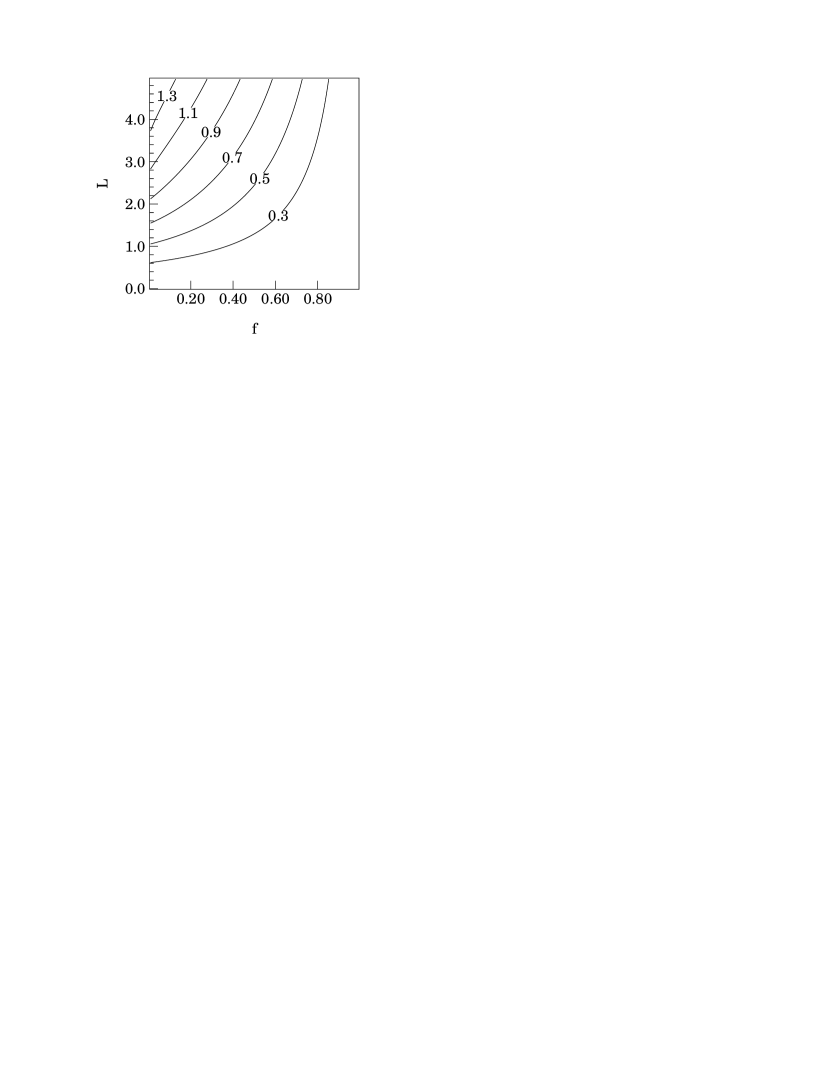
Figure A1: Contours of velocity range, $\Delta\tilde{v}=\frac{1}{2}(|\tilde{v}_{f}-\tilde{v}_{s}|)$ for a cloud in a patchy medium characterized by filling factor, $f$, and cell length, $\tilde{L}$.

Table 1: Terminal Velocity Model Predictions for Clouds of Known Distance

Cloud	b	$v$	$N(HI)$	Predicted $z~{}(kpc)$		Observed $z$
		$km~{}s^{-1}$	$\log~{}cm^{-2}$	A	B	(kpc)
Complex M	62	$-98\pm 1$	$18.6\pm 0.1$	$3.44\pm 0.02$	$3.46\pm 0.02$	$1.5-4.1$
$G259+61-64$	61	-64.2	18.36	3.22	3.24	$<4.90$
$G22+52-43$	52	-42.9	18.91	1.69	1.84	$0.10-0.53:$
$G218-63-30$	-63	-30.3	18.45	1.68	1.84	$0.08-1.60:$
IV Arch	62	$-66.3\pm 0.3$	$18.85\pm 0.03$	$1.56\pm 0.01$	$1.74\pm 0.01$	$0.78-1.5$
$G322+55-29$	55	-28.9	18.76	1.22	1.46	$0.08-0.86$
$G113+50-71$	50	-70.9	19.77	0.96	1.26	$0.06-1.60$
$G68+64-22$	64	-21.5	19.24	0.15	0.51	$0.10-0.79$
UMa IVC	53	$-44.9\pm 0.7$	$20.2\pm 0.2$	$0.10\pm 0.02$	$0.43\pm 0.02$	$0.29\pm 0.08$
$G322+55-20$	55	-20	19.5	0.08	0.41	$0.08-0.86$

Table 2: Terminal Velocity Model Predictions for Absorption Components Seen in HD 93521 ($z=1.5\pm 0.4~{}kpc$; $b=62$)

Component	$v$	$N(SII)$	$N(SIII)$	$N(HI)_{s}$	$f_{c}$	Predicted $z~{}(kpc)$
	$km~{}s^{-1}$	$\log~{}cm^{-2}$	$\log~{}cm^{-2}$	$\log~{}cm^{-2}$		A	B
1	$-66.3\pm 0.3$	$14.09\pm 0.03$	$13.05\pm 0.21$	$18.85\pm 0.03$	0.44	$1.56\pm 0.01$	$1.74\pm 0.01$
2	$-57.8\pm 0.3$	$14.50\pm 0.02$	$13.11\pm 0.22$	$19.26\pm 0.02$	0.76	$1.00\pm 0.01$	$1.30\pm 0.01$
3	$-51.2\pm 0.7$	$14.53\pm 0.03$	$13.71\pm 0.07$	$19.29\pm 0.03$	0.43	$0.39\pm 0.02$	$0.80\pm 0.02$
4	$-38.8\pm 0.5$	$14.02\pm 0.07$	$13.14\pm 0.31$	$18.78\pm 0.07$	0.35	$0.64\pm 0.02$	$1.02\pm 0.02$
5	$-29.1\pm 0.5$	$13.16\pm 0.20$		$17.92\pm 0.20$	1.0	$2.68\pm 0.03$	$2.74\pm 0.03$
6	$-18.2\pm 0.4$	$14.51\pm 0.02$		$19.27\pm 0.02$	1.0	$0.11\pm 0.04$	$0.44\pm 0.04$
7	$-10.2\pm 0.3$	$14.66\pm 0.02$		$19.42\pm 0.02$	1.0	$0.03\pm 0.05$	$0.21\pm 0.05$

Table 3: Kinematically Derived Halo Density and Drag coefficient

Star	b	$z$	$v_{-}$	$N(HI)$	$n^{kin}_{h}(z)C_{D}f_{c}$	$C_{D}f_{c}$
		kpc	$km~{}s^{-1}$	$\log~{}cm^{-2}$	$(cm^{-3})$	A	B
HD 100340	$61$	$5.00$	$-68$	18.25	$5.19\times 10^{-4}$	5.052	5.039
HD 121968	$56$	$4.30$	$-57$	17.93	$2.99\times 10^{-4}$	1.350	1.341
BD $+38~{}2182$	$62$	$4.10$	$-98$	18.60	$5.79\times 10^{-4}$	2.096	2.078
HZ 25	$80$	$3.30$	$-84$	17.94	$2.34\times 10^{-4}$	0.351	0.342
HD 121800	$50$	$1.70$	$-91$	18.92	$8.24\times 10^{-4}$	0.213	0.172
HD 93521	$62$	$1.50$	$-66$	18.85	$1.99\times 10^{-3}$	0.415	0.314
HD 219188	$-50$	$-1.50$	$-48$	18.47	$1.03\times 10^{-3}$	0.215	0.163
HD 97991	$52$	$1.20$	$-49$	18.92	$2.91\times 10^{-3}$	0.435	0.292
HD 91316	$53$	$0.79$	$-56$	18.33	$5.66\times 10^{-4}$	0.054	0.029
HD 220172	$-63$	$-0.56$	$-35$	18.68	$4.18\times 10^{-3}$	0.309	0.122
HD 137569	$52$	$0.50$	$-35$	19.06	$6.69\times 10^{-3}$	0.464	0.159
HD 87015	$51$	$0.27$	$-30$	19.43	$1.63\times 10^{-2}$	0.878	0.151
HD 113001	$81$	$0.26$	$-35$	19.30	$1.80\times 10^{-2}$	0.958	0.159
HD 100600	$69$	$0.23$	$-37$	19.54	$2.20\times 10^{-2}$	1.133	0.164
HD 219688	$-62$	$-0.10$	$-13$	19.73	$1.26\times 10^{0}$	5.627	0.330
HD 138749	$55$	$0.07$	$-28$	19.90	$2.29\times 10^{-2}$	0.989	0.049
HD 120315	$65$	$0.04$	$-11$	19.18	$2.28\times 10^{-2}$	0.953	0.042

References

- (1) Albert, C. E. 1983, ApJ, 272, 509
- (2) Albert, C.E., Blades, J.C., Morgon, D.C., Lockman, F.J, Proulx,M., Ferrarese, L. 1993 ApJS, 88, 81
- (3) Balbus, S. A. 1988, ApJ, 328, 395
- (4) Benjamin, R.A. 1996a, in “The Physics of Galactic Halos” (Conference Proceedings of Workshop in Bad Honef), ed. Dettmar, R.J., in press.
- (5) Benjamin, R.A. 1996b, BAAS 28(3), in press
- (6) Benjamin, R.A., Hiltgen, D.D., & Sneden, C. 1997, AJ, in preparation
- (7) Benjamin, R.A., Venn, K. A., Hiltgen, D. D., & Sneden, C. 1996, ApJ, 464 836
- (8) Benjamin, R.A., & Shapiro, P.R. 1996, ApJS, submitted
- (9) Binney, J., & Tremaine, S. 1987, Galactic Dynamics (Princeton University Press: Princeton) 89
- (10) Boulares, A., & Cox, D.P. 1990, ApJ, 365, 544
- (11) Bregman, J. N. 1980, ApJ, 236, 577
- (12) Bregman, J. N., & Harrington, J. P. 1986, ApJ, 309, 833
- (13) Comeron, F., & Torra, J. 1992, A&A, 261, 94
- (14) Cox, D.P., & Reynolds, R.J. 1987, ARA&A, 25,303
- (15) Cox, D.P., & Smith, B.W. 1974, ApJ, 189, L105
- (16) Danly, L. 1989, ApJ, 342, 785
- (17) Danly, L., Albert, C.E., & Kuntz, K.D. 1993, ApJ, 416, L29
- (18) Danly, L., Lee, P., and Benjamin, R.A. 1997, ApJ, in preparation
- (19) Danly, L., Lockman, F.J., Meade, M.R., and Savage, B.D. 1992, ApJS, 81, 125
- (20) de Boer, K.S., Altan, A.Z., Bomans, D.J., Lilienthal, D., Moehler, S., Van Woerden, H., Wakker, B.P., & Bregman, J.N. 1994, A&A, 286, 925
- (21) Dickey, J.M., & Lockman, F.J. 1990, ARA&A, 28,215
- (22) Ferland, G. J. 1993, University of Kentucky Department of Physics and Astronomy Internal Report
- (23) Ferrara, A., & Einaudi, G. 1992, ApJ, 395, 475
- (24) Ferrara, A., & Field, G.B. 1994, ApJ, 423, 665
- (25) Field, G.B. 1965, ApJ, 142, 351
- (26) Field, G.B., & Saslaw, W.C. 1965, ApJ, 142, 568
- (27) Foote, G.B., & du Toit, P.S. 1969, J. Appl. Meteor., 8, 249
- (28) Garmire, G.P., Nousek, J.A., Apparao, K.M.V., Burrows, D.N., Fink, R.L., & Kraft, R.P. 1992, ApJ, 399, 694
- (29) Jenkins, E. B. 1987, in Interstellar Processes, ed. Hollenbach, D.J. and Thronson, H.A., Jr (Reidel: Dordrecht) 533.
- (30) Jones, T.W., Kang, H, & Tregillis, I.L. 1994, ApJ, 432, 194
- (31) Jones, T.W., Ryu, D. & Tregillis, I.L. 1997, ApJ, in press
- (32) Kaelble, A., de Boer, K.S, Grewing, M. 1985, A&A, 143, 408
- (33) Klein, R.I., McKee, C.F., and Colella, P. 1994, ApJ, 420, 213
- (34) Kuntz, K.D., & Danly, L. 1996, ApJ, 457, 703
- (35) Lepine, J.R.D., & Duvert, G. 1994, A&A, 286, 60
- (36) Li, F., & Ikeuchi, S. 1992, ApJ, 390, 405
- (37) MacLow, M.-M., & McCray, R. 1988, ApJ, 324, 776
- (38) MacLow, M.-M., McKee, C.F., Klein, R.I., Stone, J.M., Norman, M.L. 1994, ApJ, 433, 757
- (39) McKee, C. 1993, in Back to Galaxy: AIP Conference Proceedings, ed. Holt, S.S. & Verter, F. (New York: American Institute of Physics), 499
- (40) McKee, C. & Ostriker, J.P. 1977, ApJ, 218, 148
- (41) Muller, C.A., Oort, J.H., & Raimond, E. 1963, C.R. Acad. Sci Paris 257,1661
- (42) Munch, G., & Zirin, H. 1961, ApJ, 133,11
- (43) Norman, C. A., & Ikeuchi, S. 1989, ApJ, 345, 372
- (44) Odenwald, S.F., 1988, ApJ, 325, 320
- (45) Oort, J.H., 1954, B.A.N. 12, 177
- (46) Rand, R.J. 1997, ApJ, in press
- (47) Rand, R.J., & Stone, J.M. 1996, AJ, 111,190
- (48) Reynolds, R.J. 1993, in Back to the Galaxy: Proceedings of 3rd Annual Astrophysics Conference in Maryland: AIP Conf. Series No. 278 (ed. S.S. Holt & F. Verter) (AIP Press), p 156.
- (49) Reynolds, R.J. 1989, ApJ, 339, L29
- (50) Shapiro, P.R., & Field, G.B. 1976, ApJ, 205, 762
- (51) Songaila, A., Cowie, L.L., & Weaver, H. 1988, ApJ, 329, 580
- (52) Spergel, D.N., 1994, priv. communication to M. Wolfire.
- (53) Spitzer, L., Jr. 1956, ApJ, 124, 20
- (54) Spitzer, L., Jr. 1990, ARA&A, 28, 71
- (55) Spitzer, L., Jr., & Fitzpatrick, E.L. 1993, ApJ, 409, 299
- (56) Snowden, S. L., Hasinger, G., Jahoda, K., Lockman, F. J., McCammon, D. & Sanders, W. T. 1994, ApJ, 430, 601
- (57) Tenorio-Tagle, G., Franco, J., Bodenheimer, P., and Rozyczka, M. 1987, A&A, 179, 219
- (58) Wakker, B. P. 1990, PhD thesis, Groningen
- (59) Wakker, B.P., & Schwarz, U.J. 1991, A&A, 250, 484
- (60) Weiner, B.J., & Williams, T.B. 1996, AJ, 111, 1156
- (61) Weisberg, J.M., Rankin, J.M., & Boriakoff, V. 1987, A&A, 186, 307
- (62) Wesselius, P.R., & Fejes, I. 1973, A&A, 24, 15
- (63) Wolfire, M.G., McKee, C.F., Hollenbach, D., & Tielens, A.G.G.M. 1995, ApJ, 453, 673
- (64)