SUSX-TH-96-020 astro-ph/9612135
Scaling and Small Scale Structure in Cosmic String Networks

Abstract

We examine the scaling properties of an evolving network of strings in Minkowski spacetime and study the evolution of length scales in terms of a 3-scale model proposed by Austin, Copeland and Kibble (ACK). We find good qualitative and some quantitative agreement between the model and our simulations. We also investigate small-scale structure by altering the minimum allowed size for loop production $E_{c}$. Certain quantities depend significantly on this parameter: for example the scaling density can vary by a factor of two or more with increasing $E_{c}$. Small-scale structure as defined by ACK disappears if no restrictions are placed on loop production, and the fractal dimension of the string changes smoothly from 2 to 1 as the resolution scale is decreased. Loops are nearly all produced at the lattice cut-off. We suggest that the lattice cut-off should be interpreted as corresponding to the string width, and that in a real network loops are actually produced with this size. This leads to a radically different string scenario, with particle production rather than gravitational radiation being the dominant mode of energy dissipation. At the very least, a better understanding of the discretisation effects in all simulations of cosmic strings is called for.

^(a)Centre for Theoretical Physics
University of Sussex
Brighton BN1 9QH
UK
^(b)Département de Physique Théorique
Université de Genève
Quai Ernest-Ansermet 24
CH-1211 Genève 4
Switzerland

1 Introduction

Cosmic strings formed during a cosmological phase transition at an energy scale of about $10^{16}$ GeV are sufficiently massive to seed structure formation. However, calculations of the gravitational effects from strings are hampered by uncertainty over the statistics of the evolving network [1, 2].

From lattice simulations of string formation [3], a picture has developed of a string network at formation consisting of a scale-invariant distribution of closed loops together with a percentage of infinite brownian strings crossing the Universe. The subsequent evolution would consist of the growth of the step length of the brownian infinite string network as the strings attempt to straighten out, and energy loss via loop production during reconnection.

Early analytic work identified the key property of scaling where at least the gross properties of the network can be characterised by a length scale, roughly the persistence length or the interstring distance $\xi$, which grows with the horizon [4]. This result was supported by subsequent numerical work [5]. However, further investigation revealed dynamical processes, including loop production, at scales much smaller than $\xi$ [6, 7]. In response, Austin et al developed a model describing the network in terms of three scales [8] (hereafter ACK). These scales are: the usual energy density scale $\xi$, a correlation length $\bar{\xi}$ along the string and a scale $\zeta$ relating to local structure on the string. It seemed likely from the ACK model that $\xi$ and $\bar{\xi}$ would scale with $\zeta$ growing slowly, if at all, until gravitational radiation effects became important when $\zeta/\xi\approx 10^{-4}$ [9]. Progress has also been made using alternative analytical approaches in [10, 11].

Understanding how the network scales is important because it simplifies the process of building a model representing the evolving network. Predictions of the power in the anisotropies in the Microwave Background require the two-time correlation functions for various components of the string energy-momentum tensor evolving over $O(10^{3}-10^{4})$ expansion times. As present simulations cannot achieve this range, constructing a model is necessary. We presented a simple model of the two-time correlation functions in a non-expanding background in [12].

In this paper we present the results of a numerical study of evolving strings in a Minkowski space-time. We demonstrate the scaling behaviour of correlation functions of ${\bf p}$ and ${\bf q}$ vectors (dynamical quantities which are linear combinations of tangent and velocity vectors) along the string. These functions may be used to complement analytical studies [8] and also in existing formalism to predict small-scale anisotropy in the cosmic microwave background [13]. The largest length scale associated with these correlations, $\bar{\xi}$, and the interstring distance $\xi$ are both significantly smaller than the causal horizon which suggests that the effects of the expanding background on the correlation functions are small. Following Coulson et  al  [14], we think of the Minkowski network of strings as modelling more realistic strings, by mapping Minkowski time to conformal time and Minkowski space to comoving coordinates.

As a test for the ACK model, we examine the rate equations for the evolving length scales developed in ACK as they apply to a Minkowski space-time with no gravitational radiation, and compare the results with our simulations. Such a comparison is problematic because there are a number of parameters which are difficult to calculate directly. In particular, the parameter $k$ which controls the behaviour of $\zeta$ is hard to measure. We have showed good quantitative agreement between the ACK model and our simulations for the approach to scaling of $\xi$, and qualitative agreement for $\zeta$.

A major problem is understanding the relationship between small-scale structure along the string and loop production. Bennett and Bouchet [6] provide evidence that strings possess a fractal substructure arising from kink production during reconnection. This “intermediate” fractal, constant at fixed time, spreads over a larger range of scales as the network evolves and by the end of the simulation covers a range between the resolution scale and the persistence length $\bar{\xi}$. Most of the loop production occurs at scales near the resolution scale. Shellard and Allen [6] also observe loop production near the scale of resolution and an “intermediate” fractal in the long string, although they attribute the fractal to the effect of initial conditions and a restrictive dynamical range.

The build up of small-scale structure is allowed by the Austin et  al  analysis: their original guesses for the model parameters yield the increase in small-scale structure observed in the expanding Universe codes. However, it is not well known that their model can also predict that the small-scale structure (as measured by $\zeta$) is absent.

Indeed, we find that if there are no restrictions on loop production, then small-scale structure will disappear: all three length scales defined in ACK will have the same magnitude. We also find that the region of constant fractal dimension, which we observe if we artificially constrain loop production, disappears. This has interesting implications for the energy loss mechanism from cosmic strings.

The standard scenario is that any build up of small-scale structure will only be checked by the back reaction from the string’s own gravitational field, which only becomes effective when $\zeta/\xi$ is small (of order $10^{-4}$) [9]. Loop production will then grow with the horizon, albeit at a scale much smaller than $\xi$. Although much smaller than $\xi$, these loops are vastly bigger than the string width and will be topologically stable, losing energy through gravitational radiation.

If there is no small-scale (as measured by $\zeta$) and loop production occurs at the smallest possible scale - presumably the string width - then energy loss will be dominated by production of GUT quanta [15]. Furthermore, particle production from cuspy regions may occur without any conventional loop production at all. This will obviously allow the string scenario to avoid any gravity wave bounds [1], but the implications for the decay products of the string quanta are less clear. Recent calculations of the flux of high energy decay products from string quanta have been compared with observed fluxes to put an upper bound on the proportion of string energy going into particles [16]. In the standard scenario these bounds can be avoided [17]. However, if energy loss is dominated by particle production such bounds will constrain the GUT physics if the GUT scale string scenario is to survive.

2 Algorithm and Code

In Minkowski space the string equations of motion are

$${\bf X}^{\prime\prime}=\ddot{\bf X},$$ (1)

where $\dot{\bf X}={\partial{\bf X}/\partial\eta}$ and ${\bf X}^{\prime}={\partial{\bf X}/\partial{s}}$; $\eta$ is time and ${s}$ is a space-like parameter along the string. The spatially flat FRW metric is conformal to the Minkowski metric and we regard the Minkowski time as conformal time, in the limit that the expansion of the Universe goes to zero.

${\bf X}={\bf X}({s},\eta)$ is a position three-vector which satisfies the constraints

$${\bf X}^{\prime}\cdot\dot{\bf X}=0,$$ (2)

$${\bf X}^{\prime 2}+\dot{\bf X}^{2}=1.$$ (3)

The first constraint ensures no tangential velocities, and (3) ensures that the energy of a segment of string is proportional to its length when measured in units of $s$.

Using a development of a code written by one of us previously [7, 18], we solve the wave Eq. (1) with the Smith-Vilenkin algorithm [19]. This algorithm uses the exact finite difference solution to (1),

$${\bf X}({s},\eta+\delta)={\bf X}({s}+\delta,\eta)+{\bf X}({s}-\delta,\eta)-{\bf X}({s},\eta-\delta).$$ (4)

If the string points are initially defined on the sites of a cubic lattice $(N\delta)^{3}$, then (4) ensures that they remain on the lattice at time steps of $\delta$. The discretised gauge conditions require that for these initial conditions, string links are restricted to three types: stationary (${|{\bf\dot{X}}|}=0$,  ${|{\bf X^{\prime}}|}=1$), diagonal (${|{\bf\dot{X}}|}=1/\sqrt{2}$,  ${|{\bf X^{\prime}}|}=1/\sqrt{2}$) and cusps (${|{\bf\dot{X}}|}=1$,  ${|{\bf X^{\prime}}|}=0$).

Because the string points lie on the sites of the lattice, identifying crossing events is simple. When two strings cross, they intercommute with a probability which is set to $P_{I}$. For most of this work we set $P_{I}=1$, subject to the condition that reconnection does not create a loop smaller than the threshold $E_{c}$. Loops with energy greater than or equal to a threshold value of $E_{c}$ are allowed to leave the network, while reconnections are forbidden for loops with energy equal to $E_{c}$. Forbidding reconnections allows energy to leave the network fairly efficiently; otherwise it takes much longer for the effect of the initial conditions to wear off. This feature may also model more realistic networks as, in an FRW Universe, small loops will decouple from the expansion and are highly unlikely to reconnect.

An interesting value for $E_{c}$ is the minimum segment length $2\delta$. The loops produced in this case are “cusps”: confined to one lattice site and travelling at the speed of light. The cutoff then becomes a lattice cutoff.

The ability to alter $E_{c}$ allows us a certain amount of control over small-scale structure and related quantities. For example, as $E_{c}$ is increased from $2\delta$ to $8\delta$, the rms velocity of a segment along the string increases from $0.36$ (very close to the matter era value in Bennett and Bouchet) to $0.46$ (close to the radiation era value). This corresponds to a build up of fast-moving small-scale structure.

Initial string configurations are generated using the Vachaspati-Vilenkin algorithm [3], which mimics the breaking of a $U(1)$ symmetry during a cosmological phase transition. In this approach, phases from the minimally discretised $U(1)$ group are placed randomly on the sites of a cubic lattice. Strings (or anti-strings) are identified as passing through a face with a net winding about the manifold. The strings are then joined up within the lattice cells to from a network (any ambiguity if two strings leave and two strings enter a lattice cell is settled randomly). The domains, and consequently the initial network step size $\xi_{0}$, are of constant size. This initial configuration is defined on a cubic lattice with fundamental lattice spacing $\delta$. We can alter the initial correlation length $\xi_{0}$ in terms of $\delta$. If each initial segment length is made up of a large number of individual stationary string links, peculiarities arise in the scaling solution as entire segments can be annihilated into loops of energy $E_{c}$ moving at the speed of light. Consequently we add structure in the form of cusps to break up long straight segments. Cusps are string links confined to one lattice site which move at the speed of light. Figures 1 and 2 show a Vachaspati-Vilenkin string network shortly after formation and after a period of evolution.

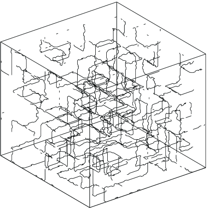
Figure 1: Strings formed with the Vachaspati-Vilenkin algorithm in a $(128\delta)^{3}$ box with $\xi_{0}=8\delta$. This snapshot is taken shortly after formation.

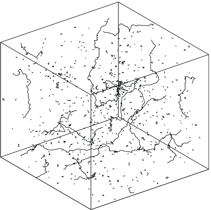
Figure 2: The strings pictured in the previous figure after the evolution period with $E_{c}=4\delta$.

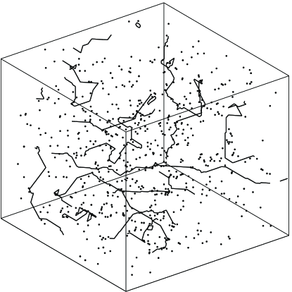
Figure 3: The strings pictured in Figure 1 after the evolution period with $E_{c}=2\delta$. The number of small loops is suppressed.

We have studied simulations on lattices ranging from $(64\delta)^{3}$ to $(1024\delta)^{3}$ . We varied $\xi_{0}$ from $8\delta$ to $64\delta$ and $E_{c}$ from $2\delta$ to $8\delta$. Periodic boundary conditions are imposed throughout. We restrict the evolution time to half the box size, as after this time causal influences have propagated around the box.

An ensemble typically consists of 30-50 runs. Unless otherwise stated, measurements were taken from networks created in a $(128\delta)^{3}$ box with $\xi_{0}=8\delta$.

3 Left and right movers

The most general solution to Eq. (1) for cosmic strings in a Minkowski spacetime is

$${\bf X}({s},\eta)={1\over 2}[{\bf a}({s}-\eta)+{\bf b}({s}+\eta)].$$ (5)

This solution may be considered as made up of “left-moving” (${\bf a}$) and “right-moving” (${\bf b}$) pieces. We will consider the dynamical quatities ${\bf p}$ and ${\bf q}$ defined

$${\bf p}={\bf b^{\prime}}=\dot{\bf X}+{\bf X}^{\prime},$$ (6)

$${\bf q}=-{\bf a^{\prime}}=\dot{\bf X}-{\bf X}^{\prime},$$ (7)

where ${\bf p}^{2}={\bf q}^{2}=1$. The solution (5) may then be represented by a pair of curves for ${\bf p}$ and ${\bf q}$ on a unit (“Kibble-Turok”) sphere. String intercommutation can excise a loop between ${s}_{1}$ and ${s}_{2}$ if

$$\int_{{s}_{1}}^{{s}_{2}}d{s}({\bf p}-{\bf q})=0.$$ (8)

At such an intercommutation event, kinks are created as abrupt changes in the ${\bf p}$ and ${\bf q}$ vectors. Left and right moving kinks travel away from the intercommutation site in opposite directions. Correlations between ${\bf p}$s and ${\bf q}$s along the string are extremely important [8, 13] as they relate to loop production, but cannot easily be calculated a priori. If ${s}={s}_{1}-{s}_{2}$

$$C_{pp}(s,\eta^{\prime})=\langle{{\bf p}(s_{1})\cdot{\bf p}(s_{2})\rangle}|_{\eta=\eta^{\prime}},$$ (9)

$$C_{pq}(s,\eta^{\prime})=\langle{{\bf p}(s_{1})\cdot{\bf q}(s_{2})\rangle}|_{\eta=\eta^{\prime}},$$ (10)

These two correlation functions contain all the information needed as $C_{qq}(s)=C_{pp}(s)$ and $C_{qp}(s)=C_{pq}(-s)$. We find that these functions approximately scale with $\xi$ i.e. they are functions of $s/\xi$ only. We calculated these correlation functions over an ensemble of 50 realisations for various $E_{c}$. The results for the scaling functions for $E_{c}=2\delta$ are plotted in Figure (4). The ensemble averages are fitted well by the simple functions:

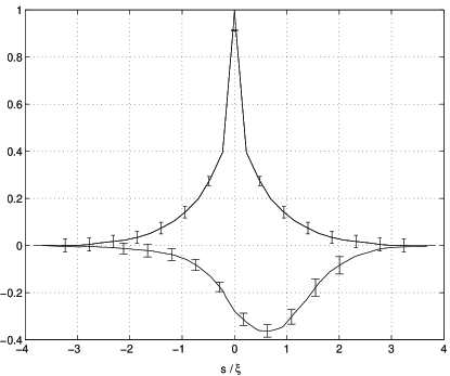
Figure 4: Scaling $C_{pp}$ (upper curve) and $C_{pq}$ correlation functions for $\xi_{0}=8\delta$ and $E_{c}=2\delta$.

$$C_{pp}(|s|/\xi)=(1-\omega)e^{-a|s|/\xi}+\omega e^{-b|s|/\xi},$$ (11)

$$C_{pq}(s/\xi)=de^{-f(s/\xi-e)^{2}}.$$ (12)

The first of these was used in [8] for demonstration purposes, but is in fact a good approximation to our measurements. It is particularly good for the $E_{c}=2\delta$ case. The gaussian form for $C_{pq}$ becomes less good away from the peak as the tail may become exponential. The gaussian fit is however within the ensemble errors.

parameter	$E_{c}=2\delta$	$E_{c}=4\delta$	$E_{c}=8\delta$
$\omega$	0.57 $\pm$ 0.05	0.45 $\pm$ 0.03	0.25 $\pm$ 0.03
$a$	5.4 $\pm$ 1.2	20 $\pm$ 3	-
$b$	0.54 $\pm$ 0.1	0.35 $\pm$ 0.04	0.17 $\pm$ 0.03
$d$	-0.34 $\pm$ 0.02	-0.20 $\pm$ 0.02	-0.08$\pm$ 0.02
$f$	0.55 $\pm$ 0.1	0.30 $\pm$ 0.05	0.03 $\pm$ 0.01
$e$	0.70 $\pm$ 0.1	1.1 $\pm$ 0.1	3.8 $\pm$ 0.2

Table 1: Parameters for model $C_{pp}$ and $C_{pq}$ functions.

The parameters for the model functions are given in Table 1. The parameters $a$ and $b$ pick out two length scales along the string. The effect of increasing $E_{c}$, and therefore small scale structure, is to decrease the small scale $1/a$ and increase the large scale $1/b$, relative to $\xi$. However, for $E_{c}>4\delta$ the small scale set by $1/a$ is no longer constant and $C_{pp}$ and $C_{pq}$ do not truly scale.

The related correlations between the tangent and velocity vectors along the string are shown in Figure 5.

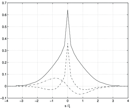
Figure 5: The scaling functions for correlations between the following vectors: tangent-tangent ($-$), velocity-velocity ($-\,-\,$) and tangent-velocity ($-\,\cdot$) for $\xi_{0}=8\delta$ and $E_{c}=2\delta$.

These functions can be calculated as simple sums of (11) and (12) using equations (6) and (7).

4 Length scales and rate equations

Analytic work as so far led to three dynamical length scales characterising the network. Austin, Copeland and Kibble [8] have considered network evolution in terms of the dynamics of left- and right-moving kinks and have defined three length scales used in their analysis which we can calculate using our simulations:

(i) $\xi$, the familiar energy density length scale

(ii) $\bar{\xi}$, a persistence length along the string

(iii) $\zeta$, a measure of the small-scale kinky structure. Their definitions are

$$\xi(\eta) = \sqrt{\mu/\rho_{l}(\eta)},$$ (13)

$$\bar{\xi}(\eta) = \int\limits_{0}^{\infty}ds\langle{{\bf p}(s_{1}).{\bf p}(s_{2})\rangle},$$ (14)

$$= ((1-\omega)/a+\omega/b)\xi,$$ (15)

$$\zeta^{-1}(\eta) = -1/{\partial\over\partial s}\langle{{\bf p}(0).{\bf p}(s)\rangle}|_{s=0},$$ (16)

$$= ((1-\omega)a+\omega b)\xi^{-1},$$ (17)

where $\xi$ and $\bar{\xi}$ are also expressed in terms of the specific correlation function given in (11).

The angular brackets $\langle{\rangle}$ indicate averaging over the long string, which is defined as all string having energy greater than $\xi$, and over an ensemble of realisations.

ACK developed rate equations for the three length scales. From their (expanding universe) analysis it seemed most likely that the network would enter a transient scaling regime, in which $\xi$ and $\bar{\xi}$ scaled but $\zeta$ did not. ($\zeta$ would scale only after gravitational back reaction was taken into account, when ${\zeta/\bar{\xi}}\approx 10^{-4}$) . In order to study this solution, we considered these rate equations and made an approximation suitable to our simulations: we ignore terms involving Hubble expansion or gravitational radiation. Then the rate equations become:

$${\dot{\xi}\over\xi}={c\over 2\bar{\xi}},$$ (18)

$${\dot{\bar{\xi}}\over\bar{\xi}}={-\chi\bar{\xi}\over\omega\xi^{2}}+{I\over 2\bar{\xi}},$$ (19)

$${\dot{\zeta}\over\zeta}={-\chi\zeta\over\xi^{2}}+{kc\over\bar{\xi}}.$$ (20)

In Eq. (18), $c$ characterises loop production. ACK consider it as function of ratios of length scales, although it should tend to a constant in the scaling regime of our simulations. In Eq. (19), $\chi$ is a geometrical factor affecting the frequency of intercommutation between uncorrelated string segments; $\omega$ is a parameter in the correlation function $C_{pp}$ as described by Eq. (11). The function $I$ also relates to loop production. In Eq. (20), $k$ relates to the efficiency of small-scale structure removing itself from the long string network. We change variables to $x=\xi/\eta$, $\bar{x}=\bar{\xi}/\eta$ and $z=\zeta/\eta$ to express the above rate equations:

$${\eta\dot{x}}={cx\over 2\bar{x}}-x,$$ (21)

$${\eta\dot{\bar{x}}}={-\chi\bar{x}^{2}\over\omega x^{2}}+{I\over 2}-\bar{x},$$ (22)

$${\eta\dot{z}}={-\chi z^{2}\over x^{2}}+{kcz\over\bar{x}}-z.$$ (23)

5 The Approach to Scaling

As in ACK we express each length scale as the product of time and a scaling variable so that $\xi=x\eta$, $\bar{\xi}=\bar{x}\eta$ and $\zeta=z\eta$. It has been widely reported [5, 6, 7] that $\xi$ scales.

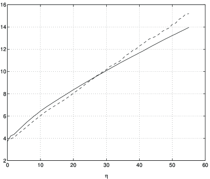
Figure 6: Plot of $\xi$ and $\bar{\xi}$ for a $(128\delta)^{3}$ box with $\xi_{0}=4\delta$ and $E_{c}=2\delta$.

Inspection of Figure 6 indicates the possibility that $\xi$ and $\bar{\xi}$ are not in fact scaling, but growing with a power of $\eta$ less than 1. A correction to the standard scaling scenario is also suggested by a recent analytical calculation [10]. A study of the exponent $n$ in $\eta^{n}$ as the network evolves shows that it is indeed tending towards $1$ throughout the simulations. At late times we find no significant departure from the scaling value $n=1$. For a $(128\delta)^{3}$ box, $n=0.96\pm 0.05$ which may indicate than $\xi$ is still on an approach to scaling. However, as the box size is increased, $n$ becomes ever closer to 1 with $n=1.000\pm 0.003$ for a $(1024\delta)^{3}$ box. The errors on $\bar{\xi}$ are larger, but similar conclusions apply. To extract the scaling values for the two length scales, we fit the data $\xi/\eta$ towards the end of the simulation to $x_{*}+\xi_{*}/\eta$, where $\xi_{*}$ and $x_{*}$ are free. This is motivated in part by the approach to scaling predicted from the ACK model at the end of this section.

The resulting scaling values $x_{*}$ and $\bar{x}_{*}$ are given in Tables 2 and 3. The figures are given with 1-sigma error bars from averaging over an ensemble of realisations.

$\xi_{0}$	$E_{c}=2\delta$	$E_{c}=4\delta$	$E_{c}=8\delta$
$8\delta$	0.174 $\pm$ 0.018	0.130 $\pm$ 0.012	0.089 $\pm$ 0.006
$16\delta$	0.170 $\pm$ 0.010	0.141 $\pm$ 0.010	0.109 $\pm$ 0.004
$32\delta$	0.171 $\pm$ 0.011	0.147 $\pm$ 0.006	0.117 $\pm$ 0.006
$64\delta$	0.173 $\pm$ 0.011	0.144 $\pm$ 0.003	$0.122\pm 0.014$

Table 2: Scaling values for $x=\partial\xi/\partial\eta$.

$\xi_{0}$	$E_{c}=2\delta$	$E_{c}=4\delta$	$E_{c}=8\delta$
$8\delta$	0.19 $\pm$ 0.04	0.13 $\pm$ 0.03	0.070 $\pm$ 0.03
$16\delta$	0.20 $\pm$ 0.04	0.17 $\pm$ 0.03	0.10 $\pm$ 0.03
$32\delta$	0.19 $\pm$ 0.03	0.17 $\pm$ 0.03	0.12 $\pm$ 0.04
$64\delta$	0.25 $\pm$ 0.04	0.21 $\pm$ 0.04	$0.14\pm 0.03$

Table 3: Scaling values for $\bar{x}=\partial\bar{\xi}/\partial\eta$.

The scaling parameter $x_{*}$ is independent of $\xi_{0}$, within ensemble errors. It is however strongly dependent on $E_{c}$ to the extent that, with an increase of $E_{c}$ from $2\delta$ to $8\delta$, the scaling density increases by a factor of 2. The scaling values of $\bar{x}_{*}$ have bigger ensemble errors, and this may hide some dependence on $\xi_{0}$. However, the results so far show that, within the ensemble errors the only dependence is on $E_{c}$.

One of the problems testing the model is the difficulty in calculating the parameters directly. We must use the model to calculate some of the parameters and see whether this gives consistent results. Assuming that $c$, $I$, $\chi$ and $k$ achieve scaling values then the following expressions are stable fixed points.

$$\bar{x}_{*}={c\over 2},$$ (24)

$$x_{*}=\sqrt{{\chi c^{2}\over 2\omega(I-c)}},$$ (25)

$$z_{*}=\left\{\begin{array}[]{ll}(2k-1)x_{*}^{2}/\chi&{\rm if}\>2k-1>0\\ 0&{\rm if}\>2k-1\leq 0.\\ \end{array}\right.$$ (26)

We are able to calculate $c$ directly from the scaling value of $\bar{\xi}_{*}$. The value of $\chi$ can be measured by counting the number of long string intercommutation events over each time step. Following ACK, the probability of a segment of length $\bar{\xi}$ intercommuting in a time step $\delta$ is given by:

$${\chi\bar{\xi}\delta\over\xi^{2}}.$$ (27)

We assume that the number of segments in the volume V is given by $V/(\xi^{2}\bar{\xi})$, thus the number of long string intercommutating events in a volume V over $\delta$ is given by:

$${\chi V\delta\over\xi^{4}}.$$ (28)

Figure 7 shows the number of long string intercommutations as a function of $\xi$ for $E_{c}=2\delta$, together with a slope giving an $\xi^{-4}$ dependence. From the $y$-intercept we can estimate $\chi$ at $0.05\pm 0.015$ for both $E_{c}=2\delta$ and $E_{c}=4\delta$.

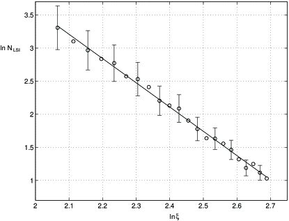
Figure 7: The number of long string intercommutation events ($N_{LSI}$) in the simulation box at each timestep plotted against $\xi$.

We are now able to make a direct test of the rate equations by considering the approach to scaling of $\xi$.

Expanding about the fixed points gives (to first order) a matrix equation equivalent to Eqs. (21)-(23):

$$\eta\dot{y}=My,$$ (29)

where

$$y=\left(\matrix{x-x_{*}\cr\bar{x}-\bar{x}_{*}\cr z-z_{*}\cr}\right),$$ (30)

and

$$M=\left(\matrix{{c\over 2\bar{x}_{*}}-1&{-cx_{*}\over 2\bar{x}_{*}^{2}}&0\cr{2\chi\bar{x}_{*}^{2}\over\omega x_{*}^{3}}&{-2\chi\bar{x}_{*}\over\omega x_{*}^{2}}-1&0\cr{2\chi z_{*}^{2}\over x_{*}^{3}}&{-kcz_{*}\over\bar{x}_{*}^{2}}&{-2\chi z_{*}\over x_{*}^{2}}+{kc\over\bar{x}_{*}}-1\cr}\right).$$ (31)

Using the scaling value for $\bar{x}_{*}$ and $\bar{z}_{*}$ given above M reduces to

$$\left(\matrix{0&{-x_{*}\over\bar{x}_{*}}&0\cr{2\chi\bar{x}_{*}^{2}\over\omega x_{*}^{3}}&{-1-{2\chi\bar{x}_{*}\over\omega x_{*}^{2}}}&0\cr{2\chi z_{*}^{2}\over x_{*}^{3}}&{-kcz_{*}\over\bar{x}_{*}^{2}}&-|2k-1|\cr}\right).$$ (32)

The eigenvalues are then $-1$, ${-2\chi\bar{x}_{*}\over\omega x_{*}^{2}}$ and $-|2k-1|$. Thus we expect in the approach to scaling (for large $\eta$) the time dependences:

$$x(\eta)=C_{1}{x_{*}\over\bar{x}_{*}}\eta^{-1}+C_{2}{\omega x_{*}^{3}\over 2\chi\bar{x}_{*}^{2}}\eta^{\epsilon}+x_{*},$$ (33)

$$\bar{x}(\eta)=C_{1}\eta^{-1}+C_{2}\eta^{\epsilon}+\bar{x}_{*},$$ (34)

$$z(\eta)=C_{3}\eta^{\lambda}+z_{*},$$ (35)

where

$$\epsilon=-2\chi\bar{x}_{*}/\omega x_{*}^{2},$$ (36)

$$\lambda=-|{2k-1}|.$$ (37)

To compare with the simulations, we measured $x=\xi/\eta$. As predicted from (33), we measured a $\eta^{-1}$ dependence for large $\eta$, although this arises partly from $\xi_{0}/\eta$. We subtract the $x_{*}+a\eta^{-1}$ dependence from a plot of $x$, leaving a term proportional to $\eta^{\epsilon}$. The resulting log-log plot for a simulation with $\xi_{0}=4\delta$ and $E_{c}=2\delta$ is shown in Figure (8), and it gives a good single power law fit to $\epsilon={-1.4}$. The ACK model predicts $\epsilon=-1.5\pm 0.2$, from Eq. (36) and our measured values for $\bar{x}_{*}$, $x_{*}$ and $\omega$. Similarly for $E_{c}=4\delta$ we measure $\epsilon=-1.8\pm 0.2$ and the model predicts $\epsilon=-1.7\pm 0.2$. We see no evidence that another scale enters into the approach to scaling.

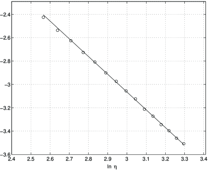
Figure 8: Log plot of the $\eta^{\epsilon}$ term in Eq. (33).

6 Small Scale Structure

Austin et  al characterise small-scale structure using ${\bf p}$ and ${\bf q}$ vectors to define a length scale, as in Eq. (17), from which we get:

$$\zeta^{-1}(\eta)=\langle{{\bf p}(0)\cdot{\bf p^{\prime}}(0)\rangle}.$$ (38)

Figure 9 shows the dependence of $\zeta$ on $E_{c}$. An $E_{c}$ of $2\delta$ allows structure to rapidly leave the network and $\zeta$ to grow. For $E_{c}=8\delta$, structure builds up on the string faster then loop production can remove it and $\zeta$ decays.

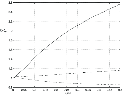
Figure 9: The behaviour of $\zeta$ for $E_{c}=2\delta$ ($-$), $E_{c}=4\delta$ ($--$) and $E_{c}=8\delta$ ($-\cdot$). The plots correspond to different box sizes to ensure that $\xi_{0}/E_{c}\geq 4$.

For $E_{c}=2\delta$ and $E_{c}=4\delta$, $\zeta$ appears to approach a scaling value. For a box of size $(128\delta)^{3}$, the exponent $n$ in $\zeta=\zeta_{*}+z\eta^{n}$ achieves $n=0.98\pm 0.03$ towards the end of the simulation and $z_{*}$ tends towards the values given in Table 4, given for a range of string densities. We note that for both these values of $E_{c}$, $\zeta/\xi\gg 10^{-4}$: much bigger than the ratio required for gravitational radiation to become significant. Indeed, for the smallest value, $\zeta$ scales at the same magnitude as $\xi$. As we increase $E_{c}$ however, we find that $\zeta$ tends towards zero growth. This signifies the build up of small-scale structure which would eventually trigger effective gravitational back-reaction. We would like to encompass the dependence of $\zeta$ on $E_{c}$ in terms of the three-scale model.

$\xi_{0}$	$E_{c}=2\delta$	$E_{c}=4\delta$
$8\delta$	$0.11\pm 0.01$	$0.007\pm 0.002$
$16\delta$	$0.12\pm 0.01$	$0.008\pm 0.002$
$32\delta$	$0.12\pm 0.01$	$0.005\pm 0.001$
$64\delta$	$0.12\pm 0.01$	$0.005\pm 0.002$

Table 4: Scaling values for $z_{*}=\partial\zeta/\partial\eta$.

The ACK model for $\zeta$, Eq. (20), consists of two processes. The first is the effect of long string intercommutation. This will serve to create kinky structure and tends to decrease $\zeta$. The second term involves the effect of small loop production. It is controlled by a parameter $k$ which reflects the extent to which loop production can remove small scale structure. If we assume a scaling regime for $\xi$ and $\bar{\xi}$ we can integrate Eq. (23) to get

$$z(\eta)={(2k-1)\eta^{2k-1}\over{C+\chi\eta^{2k-1}x_{*}^{-2}}},$$ (39)

where $C$ is a constant of integration. The evolution of $\zeta$ is then crucially dependent on $k$. For $k>\frac{1}{2}$, $\zeta$ has a positive gradient and $z$ tends towards the scaling value $z_{*}=(2k-1)x_{*}^{2}/\chi$. For $k<\frac{1}{2}$, $\zeta$ has a negative gradient and tends towards 0. From Figure 9 we see that both cases occur in our simulations, depending on the value of $E_{c}$. The three-scale model is certainly capable of explaining our simulations, if we consider $E_{c}$ as being related to $k$. This should not surprise us, as increasing $E_{c}$ artificially keeps structure on the string that would otherwise leave the network. Unfortunately, we cannot calculate $k$ a priori. We can only assume that the rate equations from the three-scale model are broadly correct and extract a value for $k$ numerically, by using the scaling expression for $z_{*}$. This gives $k=0.59$ ($E_{c}=2\delta$), $k=0.51$ ($E_{c}=4\delta$) and $k<\frac{1}{2}$ ($E_{c}>6\delta$).

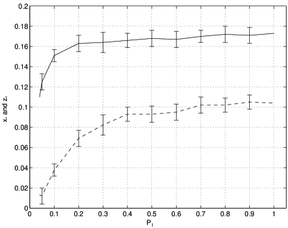
Figure 10: How the scaling values $x_{*}$ and $z_{*}$ vary with the intercommutating probability.

The effect of changing the intercommutating probability on $z_{*}$ is broadly similar to the effect of $x_{*}$ [7]. We compare the two in Figure 10. The value for $z_{*}$ changes slowly until $P_{I}\approx 0.35$ when it falls rapidly. After this point $\zeta$ is probably not scaling.

Another way to characterise small-scale structure along the string is through the relationship

$$E=R^{d},$$ (40)

where $E$ is the average energy between two points separated by a physical distance $R$. The exponent $d$ is scale dependent. On large scales it is shown in [6, 7] that $d$ tends to $2$, as the strings become random walks. On small-scales, the string becomes straight on average, and $d$ tends to 1. One might expect a smooth interpolation between these two regimes, but Bennet and Bouchet [6] note that an “intermediate” fractal $d_{i}$ (i.e. a constant or very slowly varying $d$) exists on scales between the numerical cutoff and below $\xi$. They explain this as the build up of small scale structure on over the scales of constant fractal.

Allen and Shellard [6] observe a similar structure, although they attribute it to artificial initial conditions and lack of dynamical range. We observe that this intermediate fractal exists for energy cut-offs of $8\delta$ and above whereas for $E_{c}=2\delta$ it has disappeared completely leaving a smooth transition from $d=1$ to $d=2$. This is shown in Figure 11, which is plotted for comparison with similar figures in [6]. However, it is not clear that small scale structure always reveals itself through a constant $d_{s}$. As a comparison, we calculated $E/R$ from the tangent-tangent correlation function $\langle{{\bf X^{\prime}}(z)\cdot{\bf X^{\prime}}(0)\rangle}$ with the parameters in Table 1 for $E_{c}=2\delta$. For these model parameters, we find that $\zeta\approx 0.4\xi$: certainly not a small scale. We plot the result in Figure 12 along with the measured quantity. The agreement is good up to scales well in excess of $\xi$. (The discrepancy at larger scales may be due in part to model function underestimating the ${\bf pq}$ correlations at large $\xi$, as the gaussian form of $C_{pq}$ breaks down.) However, for small scales the agreement is good and this indicates a genuine lack of small-scale structure.

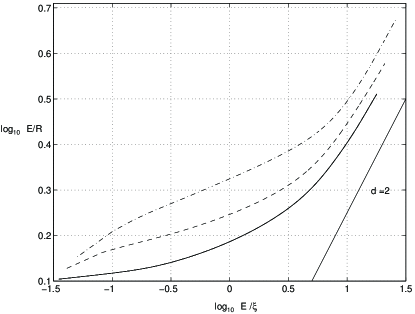
Figure 11: Log plot showing the fractal structure of the long string for energy cutoffs of $E_{c}=2\delta$ (—), $E_{c}=4\delta$ (- -) and $E_{c}=8\delta$ (-$\cdot$).

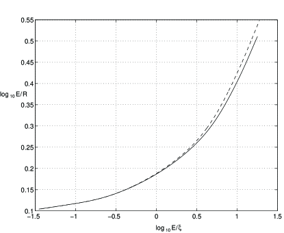
Figure 12: Log plot showing the fractal structure with a cutoff of $E_{c}=2\delta$ (—) together with the same quantity calculated from the model tangent-tangent correlation function.

7 Conclusions

We have demonstrated the scaling behaviour of correlation functions of ${\bf p}$ and ${\bf q}$ vectors, which are essential in analytic studies of string networks.

The parameters of model functions for the ${\bf pp}$ and ${\bf qq}$ correlation functions $C_{pp}$ and $C_{pq}$, depend on how much small-scale structure in present on the string, which is related to the value of the minimum allowed loop energy $E_{c}$. As $E_{c}$ is increased, small-scale structure is allowed to build up and the scaling density can increase by a factor of two more.

We analysed our simulations in terms of the three-scale model proposed by Austin et al, suitably simplified for Minkowski space with no gravitational radiation.

The model for $\xi$ describes well the approach to scaling and predicts the two exponents for this approach that we measure in our simulations. The model for the “small” scale $\zeta$ is qualitatively consistent with our simulations with critical value $k$ determining whether or not $\zeta$ will scale.

For the smallest possible value of $E_{c}$, small-scale structure disappears, as all the scales $\xi$, $\bar{\xi}$ and $\zeta$ of the 3-scale model of ACK have the same order of magnitude. Furthermore, from the fractal analysis along the string for $E_{c}=2\delta$, the transient fractal region disappears, leaving a smooth transition from straight strings on small-scales to the random walk on large scales. Thus the intermediate fractal region seen in the expanding Universe codes seems to be an effect of the limit on the size of loops.

In all cases, loops are predominantly produced at the smallest possible scale $E_{c}$, even when it is set, by the underlying lattice, to $2\delta$. Thus, in common with all other simulations (apart from those of Albrecht and Turok [5]), there is no evidence for scaling in loop production. It is therefore time to ask the question: is this the true physical situation? It is certainly possible that loops are produced with the smallest possible physical scale, which is the string width, and we see from our simulations that every other measure of the network has a single scale of order $\xi$. Thus there is no real conflict with the string scaling hypothesis.

One objection to the use of the Smith-Vilenkin algorithm is its restrictive set of possible values of ${\bf p}$ and ${\bf q}$ for the initial conditions (although the subsequent evolution is exact). As discussed by Albrecht [21], this may exaggerate small loop production. However, expanding Universe codes have no such restrictions and there is no published evidence that loop production happens at any scale other than the loop size cut-off. Furthermore, we have found no evidence that the lattice scale enters the scaling solution. If there is spurious cusp production (for $E_{c}=2\delta$) through a chance configuration of ${\bf p}$ and ${\bf q}$ vectors such that Eq. (8) is true, then one would not expect a stable scaling solution. Albrecht suggests that there may also be spurious loop production through “back-tracking” [21] which occurs when individual discretised links or groups of links point in a direction opposite to that of the whole segment of length $\xi$. In this case, one would expect the lattice scale $\delta$ to affect the evolution: for example, the rate of energy loss from back-tracking would most likely increase with $\xi/\delta$ as the chances for a given link or group of links to back-track in a time $\xi$ increases.

We are confident that our simulations do approach (and for large simulations reach) a stable scaling solution, and from Table 2 we see that the value of the scaling parameter $x_{*}$ is independent of the range of $\xi$ over which the simulation is run. We infer from this that the spurious processes mentioned above do not critically enter the observed dynamics.

The prospect that the loops are produced with such tiny sizes is a radical one. It means that the dominant mode of energy loss of a cosmic string network is particle production and not gravitational radiation as the loops collapse almost immediately. Indeed, it may not be possible to talk about loop production at all: the loop production we observe favours loops formed at cusps, which could annihilate into particles before the loop is formed [15]. Furthermore, gravitational radiation directly from a network without a small scale $\zeta\ll\xi$ is negligible.

Recent calculations [17] on the possible role of GUT quanta decaying into high energy cosmic rays assumes that particle production is subdominant to gravitational radiation as a means of energy loss, and conclude that GUT strings could not be an appreciable source of cosmic rays. In our suggested energy loss scenario, we may come up against an observational bound of high energy cosmic rays. Simple models of GUT quanta decay processes give the upper bound for the proportion of the string energy going into high energy cosmic rays as $O(10^{-3})$ or less [16]. Such calculations may put a significant constraint on GUT models if the GUT scale string scenario is to be viable.

References

- [1] M. Hindmarsh and T.W.B. Kibble Rep. Prog. Phys. 58 477 (1994)
- [2] A. Vilenkin and E.P.S. Shellard, Cosmic Strings and other Topological Defects (Cambridge University Press, Cambridge, 1994)
- [3] T. Vachaspati and A. Vilenkin Phys. Rev. D30, 2036 (1984); T. W. B. Kibble Phys. Lett. 166B, 311 (1986); K. Strobl and M. Hindmarsh to be published in Phys. Rev. E55 (1997); A recent lattice-free calculation has cast some doubt on the presence of infinite string: J. Borrill Phys. Rev. Lett. 76 3255 (1996)
- [4] T.W.B. Kibble Nucl. Phys. B252 277 (1985)
- [5] A. Albrecht and N. Turok Phys. Rev. Lett.54, 1868 (1985); A. Albrecht and N. Turok Phys. Rev. D40, 973 (1989)
- [6] D. P. Bennett, in “Formation and Evolution of Cosmic Strings”, eds. G. Gibbons, S. Hawking and T. Vachaspati, (Cambridge University Press, Cambridge. 1990); F. R. Bouchet ibid.; E. P. S. Shellard and B. Allen ibid.
- [7] M. Sakellariadou and A. Vilenkin Phys. Rev. D42 349 (1990)
- [8] D. Austin, E. J. Copeland and T. W. B. Kibble Phys. Rev. D48 5594 (1993)
- [9] M. Hindmarsh Phys. Lett. 251B 28 (1990) M. Sakellariadou Phys. Rev. D42 354 (1990)
- [10] M. Hindmarsh Phys. Rev. Lett. 77 4495 (1996)
- [11] C. J. A. P. Martins and E. P. S. Shellard Phys. Rev. D54 2535 (1996)
- [12] G. R. Vincent, M. Hindmarsh and M. Sakellariadou, to be published in Phys. Rev. D55, (1997)
- [13] M. Hindmarsh Ap. J. 431 534 (1994)
- [14] D. Coulson, P. Ferreira, P. Graham and N. Turok Nature 368 (1994)
- [15] M. Srednicki and S. Theisen Phys. Rev. B189 397 (1987)
- [16] P. Bhattacharjee and N. C. Rana Phys. Lett. 246B 365 (1990); G. Sigl, K. Jedamzik, D. N. Schramm and V. Berezinsky Phys. Rev. D52 6682 (1995)
- [17] A. J. Gill and T. W. B. Kibble Phys. Rev. D50 3660 (1994)
- [18] M. Sakellariadou and A. Vilenkin Phys. Rev. D37 885 (1988)
- [19] A. G. Smith and A. Vilenkin Phys. Rev. D36 990 (1987)
- [20] D. P. Bennett and F. R. Bouchet Phys. Rev. Lett.60, 257 (1988)
- [21] A. Albrecht, in “Formation and Evolution of Cosmic Strings”, eds. G. Gibbons, S. Hawking and T. Vachaspati, (Cambridge University Press, Cambridge. 1990).