Fabry-Perot Observations of Globular Clusters III: M15

Abstract

We have used an Imaging Fabry-Perot Spectrophotometer with the Sub-arcsecond Imaging Spectrograph on the Canada-France-Hawaii Telescope to measure velocities for 1534 stars in the globular cluster M15 (NGC 7078) with uncertainties between 0.5 and 10 $\rm{km}~{}\rm s^{-1}$. Combined with previous velocity samples, the total number of stars with measured velocities in M15 is 1597. An average seeing of 0.8″ allowed us to obtain velocities for 144 stars within 10″ of the center of M15, including 12 stars within 2″.

The velocity dispersion profile for M15 remains flat at a value of 11 $\rm{km}~{}\rm s^{-1}$ from a radius of 0.4′ into our innermost reliable point at 0.02′ (0.06 pc). Assuming an isotropic velocity dispersion tensor, this profile and the previously-published surface brightness profile can be equally well represented either by a stellar population whose M/L varies with radius from 1.7 in solar units at large radii to 3 in the central region, or by a population with a constant M/L of 1.7 and a central black hole of 1000 ${\rm M}_{\odot}$. A non-parametric mass model that assumes no black hole, no rotation, and isotropy constrains the mass density of M15 to better than 30% at a radius of 0.07 parsecs. The mass-density profile of this model is well represented by a power law with an exponent of –2.2, the value predicted by models of cluster core-collapse. Using the assumption of local thermodynamic equilibrium, we estimate the present-day mass function and infer a significant number of 0.6–0.7 ${\rm M}_{\odot}$ objects in the central few parsecs, 85% of which may be in the form of stellar remnants.

Not only do we detect rotation; we find that the position angle of the projected rotation axis in the central 10″ is 100^∘ different from that of the whole sample. We also detect an increase in the amplitude of the rotation at small radii. Although this increase needs to be confirmed with better-seeing data, it may be the result of a central mass concentration.

1 INTRODUCTION

Imaging Fabry-Perot (FP) spectrophotometers have become powerful tools for studying the dynamics of the central regions of globular clusters. The samples of individual stellar velocities that have been obtained with a FP are some of the largest available for globular clusters (Gebhardt et al. 1994, 1995, hereafter Paper 1 and Paper 2, respectively). In addition, FP observations of the integrated light at the center of a cluster provide a two-dimensional velocity map of that region with unprecedented detail. With the dramatic increase in the quality of the kinematic data available for globular clusters, more powerful analysis techniques become possible. Non-parametric techniques can provide an unbiased estimate of the dynamical state of a cluster (Merritt 1993a,b), such as the rotation and velocity dispersion properties (Paper 1 and 2). Combining the dispersion and surface brightness profiles with the Jeans equation directly yields the mass density profile and the mass function (Gebhardt & Fischer 1994, hereafter GF, Merritt & Tremblay 1994). The distribution of mass determined by this technique can be used to test the predictions of Fokker-Planck and N-body simulations.

As one of the densest nearby objects known, M15 has significant implications for the formation and evolution of dense stellar systems. It has, therefore, been the target of intense observations and theoretical modeling. Images taken with the refurbished Hubble Space Telescope (Guhathakurta et al. 1996) have shown that the luminosity density may rise all of the way into the center and do not support the core with a radius of about 2″ previously proposed by Lauer et al. (1991). Measurements of the dynamical state of M15 have also produced controversy. Is there a central cusp in the dispersion profile (Peterson, Seitzer, & Cudworth 1989), or does the profile remain flat near the center at 11 $\rm{km}~{}\rm s^{-1}$ (Paper 1, Dubath & Meylan 1994, Dull et al. 1996)? Somewhat conflicting amounts of rotation have been measured near the center by Peterson (1993) and Paper 1.

GF derived a non-parametric mass model for M15 using the velocities from Paper 1, but this has not been compared with the results of either Fokker-Planck (Grabhorn et al. 1992, Dull et al. 1996, Einsel & Spurzem 1996) or N-body (Makino & Aarseth 1992, McMillan & Aarseth 1993) evolutionary models. The strongest constraints on the models come from comparing them with the kinematics in the central few arcseconds, since this is where the effects of mass segregation, core collapse, and a possible central massive black hole are the most pronounced. Unfortunately, the uncertainties in and disagreements between the observations in this region have made comparisons difficult.

To improve our knowledge and the significance of the rotation, the value of the dispersion within 2″ of the center of M15 requires observations with higher angular resolution. The tools of crowded-field photometry can be directly applied to the two-dimensional data from a FP, making them easier to interpret for dense stellar systems than slit spectra and yielding the largest possible number of stellar velocities. Using a FP on telescopes and with instruments that provide the best seeing is a promising approach to resolving the mystery of the center of M15. This paper is the first reporting results from our study of globular cluster dynamics using data taken at the Canada-France-Hawaii Telescope (CFHT). These data have better seeing than that in Papers 1 and 2, which were taken at CTIO.

The rest of this paper is organized as follows. Sec. 2 discusses the Fabry-Perot observations and the reductions. Sec. 3 describes measurements of the first and second moments of the velocity distribution. Sec. 4 presents the mass modeling and the mass function estimates. Sec. 5 discusses the results.

2 THE DATA

2.1 Instrumentation

We used an imaging Fabry-Perot spectrophotometer with the Sub-arcsecond Imaging Spectrograph (SIS) at the CFHT on May 20–23, 1994, and May 12–17, 1995. The optical design of SIS is described in Morbey (1992) and Le Fevre et al. (1994). Light is fed to the spectrograph by a tip-tilt mirror which is driven at about 20 Hz using the signal from a quadrant detector at the focal plane in order to compensate for image motion. We placed the Rutgers narrow etalon, which has a spectral resolution of 0.8 Å FWHM at 6500 Å, in the collimated beam. This etalon is fully compatible with the CFHT etalon controller and its coatings are suitable for work at the H$\alpha$ line. The order-selecting filter was in the collimated beam below the etalon and was tilted to eliminate ghost images due to filter reflections. Before being tilted, the filter had a 16Å FWHM centered at 6569Å and a peak transmission of 83%. It was borrowed from the Dominion Astrophysical Observatory.

The SIS+FP setup provides a $3\arcmin\times 3\arcmin$ field of view. The front-side illuminated Loral3 CCD imaged this field, and we binned $2\times 2$ during readout to obtain 1024x1024 pixels at a scale of 0.173″ per pixel. The SIS guide probe is mounted on a 45″ wide arm that runs across the entire field. Fortunately, the probe’s field of view is $4\arcmin\times 3\arcmin$; with the rich star fields of globular clusters, we were able to choose V = 13 – 14 guide stars that resulted in little or no vignetting of our images by the probe. Sampling the position of the star at 40 Hz seemed adequate to follow the image motion seen on a real-time display. Fast guiding produced an approximately 15% improvement in the FWHM of the images. Thus, we were able to reduce the area of star images by about 30%, which significantly increased the number of stars for which we could obtain velocities.

2.2 Observations and Data Reduction

The FP observing and reduction procedures were the same as those described in Paper 1. We took a series of exposures stepped by 0.33 Å across the H$\alpha$ absorption line. Projector flats were obtained in the evening or morning for every wavelength setting of the etalon used that night. Approximately hourly exposures of a deuterium lamp, which provided both H$\alpha$ and D$\alpha$ emission lines, monitored the wavelength zero-point and provided the primary wavelength calibration. This calibration was supplemented by exposures of several neon lines taken throughout the run. A small offset between the focal planes of the guide probe and the SIS collimator resulted in reflections from the etalon being so out of focus that they were not detectable. We thus made no corrections for reflected light.

We obtained 17 15-minute exposures of M15 in 1994 and 15 such exposures in 1995. Frame-to-frame normalizations for non-photometric conditions, determined as described in Paper 1, were as large as a factor of two for the 1994 data. For the 1995 data, the normalizations only varied by 20%. The average FWHM of the stellar images was 0.8″ (the 1995 run) and 1.1″ (1994). The overall throughput of the system (telescope+FP+CCD) was about 15%, and for a V=16 star we were able to obtain a signal-to-noise of 18 in a 15 minute exposure under photometric conditions.

A significant change from our previous reduction procedure was employing HST images directly to assist in the photometry of the crowded central regions of M15. This was made possible by using ALLFRAME (Stetson 1994), which measures positions and brightnesses for all of the stars in a set of images simultaneously. Coordinate transformations with six coefficients map a location in one frame to the corresponding location in another. ALLFRAME makes maximum use of the positional information present in the set of frames, improving the photometry in every frame. Our initial ALLFRAME reduction used HST frames from Guhathakurta et al. (1996) and all of the frames from the 1994 and 1995 CFHT runs. Unfortunately, the line profiles resulting from this photometry were very noisy. We believe that this resulted from faint stars which are isolated in the HST images, but very blended with a brighter neighbor in the CFHT images. The partitioning of light among the crowded stars varied wildly from CFHT frame to CFHT frame. The “sky” level determined in the CFHT frames also tended to be incorrect. These problems are clearly related to the large difference in resolution between the CFHT and HST images.

A different initial list of stars to be reduced or some other change of procedure might have solved these problems. However, what we chose to do was to photometer each CFHT frame individually using ALLSTAR, but holding the positions of the stars fixed at those found from the ALLFRAME reduction. This allowed ALLSTAR to determine, based on a uniform chi-square criterion, whether there was adequate information in an individual frame to determine a star’s magnitude with acceptable precision. The line profiles produced by this procedure were smoother, but crowding probably still introduces some additional uncertainties into our velocities inside a radius of about 0.3′. This is discussed in somewhat more detail below.

We also used the HST photometry to determine which stars in the CFHT frames were sufficiently contamination by light from neighbors that their measured velocity could be affected. The criterion is based on Monte Carlo simulations and is the same as used in Paper 1. Due to the 0.8″ FWHM seeing of the CFHT SIS frames, only eight stars were excluded from the final sample.

2.3 Velocity Zero-Point and Uncertainties

Radial velocities for M15 stars were previously obtained by Peterson et al. (1989, hereafter PSC), who used the echelle spectrograph and intensified Reticon detector on the MMT, and by us (Paper 1). The present study includes 66 stars in common with PSC and 188 in common with Paper 1. Based on this overlap, both the 1994 and 1995 raw velocities are $7.4\pm 0.4$ $\rm{km}~{}\rm s^{-1}$ more negative than those of Paper 1, which were adjusted to the zero-point of PSC.

While a zero-point offset between radial velocities measured with different instruments is not surprising, this is the largest offset that we have seen for FP data. In order to investigate this further, we observed the radial velocity standards HD107328 and HD182572 during the 1995 run. These data were taken and reduced in a fashion very similar to the globular cluster stars. With only one star in the field we could not derive transparency normalizations for the individual frames, but conditions were photometric and the exposure times were only 15 s. Observations of HD107328 with the star near the center of the field on one night and 370 pixels from the center on another yielded velocities of $29.85\pm 0.03$ $\rm{km}~{}\rm s^{-1}$ and $30.35\pm 0.03$ $\rm{km}~{}\rm s^{-1}$, respectively. An observation of HD182572 on a third night with the star near the center of the field produced a velocity of $-106.79\pm 0.05$ $\rm{km}~{}\rm s^{-1}$. The quoted uncertainties are simply the uncertainties in the fitted line centroids, and may be underestimated since we do not include noise from possible transparency fluctuations.

The standard velocity for HD107328 is 36.6 $\rm{km}~{}\rm s^{-1}$ and for HD182572 is $-100.3$ $\rm{km}~{}\rm s^{-1}$ (Latham & Stefanik 1991). The differences between the three raw FP velocities and the standard velocities are $-6.75$, $-6.49$, and $-6.25$ $\rm{km}~{}\rm s^{-1}$. The mean difference is $-6.5$ $\rm{km}~{}\rm s^{-1}$, with an RMS scatter around this mean of 0.25 $\rm{km}~{}\rm s^{-1}$. This zero-point offset is probably caused by some combination of small wavelength, flatfielding, and normalization errors and a difference between the centroid of the stellar H$\alpha$ line measured by our line-fitting program and the tabulated laboratory wavelength of H$\alpha$. The scatter between the three velocity differences is satisfyingly small and argues that, whatever its cause, the velocity offset will not significantly increase the scatter within our cluster sample. The PSC velocity zero-point was based on spectra of the twilight sky, so we consider the agreement between the zero-points derived from the standards and from the M15 stars to be acceptable. We adopt the latter for the remainder of this paper.

Figure 1 plots V_Paper1–V_FP95 vs. V_Paper1. The comparison with PSC is similar and not shown here. Several binary star candidates are apparent in Fig. 1, but discussion of these is deferred to a future paper. The RMS difference measured with a bi-weight estimator, which is insensitive to a few outliers, is 5.0 $\rm{km}~{}\rm s^{-1}$ after correcting the zero-point of the 1995 data. This implies a typical velocity uncertainty of 3.5 $\rm{km}~{}\rm s^{-1}$. Comparing this to the average internal velocity uncertainty calculated from fitting the the H$\alpha$ line profile suggests that we need to add 1 $\rm{km}~{}\rm s^{-1}$ in quadrature to these internal uncertainties. This additional uncertainty could be due to the fits to the line profiles underestimating the uncertainties or to the velocity “jitter” of luminous cluster giants (Gunn & Griffin 1979, Mayor et al. 1983).

There are 461 stars with velocities from both the 1994 and 1995 data and this provides a large, homogeneous sample with which to explore the FP measurement uncertainties. We determined what value, added in quadrature to the internal uncertainties, produced the most uniform distribution of chi-square probabilities. Probabilities smaller than 5% are excluded to remove the effect of real velocity variables. This method was first employed by Duquennoy & Mayor (1991) and the approach that we used to judge uniformity is described in Armandroff et al. (1995). The best additive uncertainty was zero for the entire sample, though values as large as 1.0 $\rm{km}~{}\rm s^{-1}$ are acceptable. About 10% of the stars have probabilities under a few percent, which would be a surprisingly large fraction of real variables. The stars with smaller average measurement uncertainties had more low probabilities, suggesting that the brighter stars should have larger additive uncertainties. Limiting the sample to the 118 stars with approximate $V$ magnitudes (described in the next section) less than 15 produced an additive uncertainty of 1.4 $\rm{km}~{}\rm s^{-1}$.

This bright subsample also has about 10% of the stars with probabilities below a few percent and we noticed that a larger than expected number of these were at small radii. Focusing on the 393 stars outside of a radius of 0.4′, the most uniform probability distribution resulted from an additive uncertainty of 0.4 $\rm{km}~{}\rm s^{-1}$ for stars with any magnitude and from a value of 1.1 $\rm{km}~{}\rm s^{-1}$ for the 91 stars brighter than magnitude 15. This difference very likely reflects the well-known velocity jitter of luminous cluster giants and suggests that much of the additional uncertainty reflected in the comparisons with the Paper 1 and PSC velocities, which are mostly for brighter stars, comes from this source.

For the 68 stars with both 1994 and 1995 velocities inside a radius of 0.4′, the most uniform probability distribution results for an additional uncertainty of 3.2 $\rm{km}~{}\rm s^{-1}$. With this value, there is no evidence for an excess of stars with low probabilities. Most of these stars are brighter than a magnitude of 15.8 because of crowding, but it is still clear that the FP velocities suffer from additional uncertainty at small radii. Errors in the stellar photometry induced by crowding are almost certainly the cause. The line profiles at small radii show more scatter around the fitted profiles than do those at large radii. The PSC stars in this region are probably the brightest and least crowded. Comparing the PSC and 1995 velocities for the 26 stars in this region required an additional uncertainty for the CFHT velocities of only 0.7 $\rm{km}~{}\rm s^{-1}$.

All of the additional uncertainties described above are much smaller than the cluster dispersion and, thus, have little effect on the dynamical analyses. We have thus adopted the simple prescription of adding 1 $\rm{km}~{}\rm s^{-1}$ in quadrature to the uncertainties derived from the line profile fits for the 1994 and 1995 velocities. We have performed our dynamical analyses using an additional uncertainty of 3 $\rm{km}~{}\rm s^{-1}$ instead of 1 $\rm{km}~{}\rm s^{-1}$and find the same results. We have also performed the analyses both including and excluding those stars with small chi-square probabilities and find no difference in the results. The results presented below include these stars.

3 RESULTS

3.1 The Individual Stellar Velocities

We have combined five sets of M15 velocities: the PSC measurements and Fabry-Perot measurements from 1991 (Paper 1), 1992 (Paper 1), 1994 (this paper), and 1995 (this paper). Each star for which there was any ambiguity in the matching among datasets (either in the position or in the velocities) was examined carefully to ascertain the accuracy of its identification. Table 1 presents the mean stellar velocity for every measured M15 star. Col. 1 is the star ID; Cols. 2 and 3 are the x and y offset from the cluster center in arcseconds (measured eastward and northward, respectively, from the center given in Guhathakurta et al. 1996); Cols. 4 and 5 present the mean velocity and its uncertainty; Col. 6 gives the FP magnitude (estimated from the fitted continuum of our 3 Å of spectrum); and Col. 7 lists either the probability of the chi-square from the multiple measurements exceeding the observed value – a low probability suggests a variable velocity, though see § 2.3 – or a note which is explained below. The average velocity given was calculated weighting by the measurement variances, and the inverse of the uncertainty is the square root of the average of the individual inverse variances. The uncertainties include the 1.0 $\rm{km}~{}\rm s^{-1}$ added in quadrature that was discussed in the previous section.

The wavelength gradient with radius in the FP images (Papers 1 and 2) causes a bias in the velocity sample due to the limited wavelength coverage of the FP data. Stars at large radii and with velocities sufficiently more positive than the cluster mean will have incomplete wavelength coverage of the line, which makes the velocity impossible to measure. We therefore have to choose a radius from the center of the FP field where this effect may begin to affect the dynamical analysis. The SIS optics at CFHT produce a gradient of only 4 Å as compared to 6 Å at CTIO. As a result, we obtain a larger unbiased field at the CFHT than at CTIO for the same number of frames: 1.2′ in radius vs. 1.0′, respectively. The stars that are beyond this radius are not used in the dynamical analysis and have “bias” in the final column of Table 1. Stars determined to be non-members based on their radial velocity have “non” in the final column of Table 1.

The stars with a low probability (P$<0.01$) in Col. 7 are good candidates for stars whose velocity varies due to jitter or binary orbital motion. However, identifying binary candidates is difficult because of the complex situation with the velocity uncertainties discussed in § 2.3. We, therefore, postpone discussion of the binary candidates and the binary frequency to a future paper.

The individual velocity measurements from the 1994 and 1995 CFHT runs and from the previously published samples are given in Table 2. Col. 1 is the star ID; Cols. 2 and 3 are the velocity and uncertainty from the 1995 CFHT data; Cols. 4 and 5 are from the 1994 CFHT data; Cols. 6 and 7 are from the 1992 CTIO data (Paper 1); Cols. 8 and 9 are from the 1991 CTIO data (Paper 1); and Cols. 10 and 11 are from PSC. The uncertainties listed in Table 2 do not contain the additional uncertainty that is used in Table 1.

Recently, Dull et al. (1996) reported velocities for 132 member stars in the central 1′ of M15. We have repeat velocity measurements for all of their stars, and our average uncertainty is around 1.5 $\rm{km}~{}\rm s^{-1}$, while theirs is 4 $\rm{km}~{}\rm s^{-1}$. Because they do not list the uncertainties for the individual stars, we are unable to combine their velocities with our dataset in the same rigorous fashion. Since our uncertainties are smaller for their stars and since our dataset contains over a factor of ten more velocity measurements, the dynamical analysis will not be affected by not including their velocities.

Tables 1 and 2 contain only stars with velocity uncertainties smaller than 10 $\rm{km}~{}\rm s^{-1}$. We have determined that it is worthwhile to use stars with uncertainties as large as this, even though the velocity dispersion of the cluster is around 11 $\rm{km}~{}\rm s^{-1}$. We formed velocity samples that excluded stars with uncertainties larger than values as small as 4 $\rm{km}~{}\rm s^{-1}$. Dynamical analyses of these samples showed no significant change in the results other than an increase in the size of the confidence bands for the measured quantities when fewer stars were used. Thus, we employed the complete velocity sample in the analysis presented in this paper. Only four stars were found to be non-members due to their large velocity difference from the cluster mean velocity; they were excluded. An additional 22 stars were not used because they are at large radii where the dynamics may be biased by the limited spectral coverage. Of the remaining 1575 stars with uncertainties less than 10 $\rm{km}~{}\rm s^{-1}$, 1100 have uncertainties less than 5 $\rm{km}~{}\rm s^{-1}$and 685 less than 3 $\rm{km}~{}\rm s^{-1}$. Inside of 0.1′ we were able to measure velocities for 80% (71 of 89) of the stars brighter than V=18.

Figure 2 plots the individual stellar velocities and their uncertainties against the distance from the center of M15. This figure suggests that the local mean velocity for M15 becomes more positive in the central 0.1′. The weighted mean velocity of the 71 innermost stars is $-105.6\pm 1.3$ $\rm{km}~{}\rm s^{-1}$, while the mean velocity of the whole sample is $-107.8\pm 0.3$ $\rm{km}~{}\rm s^{-1}$. Therefore, the apparent change in velocity is significant at the 2$\sigma$ level. We have looked for calibration and/or normalization errors and are confident that these cannot produce such a large velocity shift. Comparison with previous authors also increases our confidence that our velocity measurements are not biased. Dubath & Meylan (1995) have measured velocities for 14 stars in the central 0.1′ of M15. The mean velocity for these 14 stars is $-103\pm 4$ $\rm{km}~{}\rm s^{-1}$, consistent with our measurement. We feel that the variation of the mean velocity with radius is simply due to statistical noise.

3.2 Rotation

We detect rotation in M15. Using maximum likelihood techniques to fit a sinusoid to the entire sample of individual stellar velocities as a function of their position angle yields a rotation amplitude of $2.1\pm 0.4$ $\rm{km}~{}\rm s^{-1}$. The position angle of the maximum positive rotation velocity, measured from north through east, is $197\arcdeg\pm 10\arcdeg$. Both of these values agree with our previous measurement of $1.4\pm 0.8$ $\rm{km}~{}\rm s^{-1}$ and $205\arcdeg\pm 33\arcdeg$ (Paper 1). Monte Carlo simulations show that a 2.1 $\rm{km}~{}\rm s^{-1}$ rotation amplitude is expected by chance when no rotation is present less than 0.1% of the time.

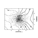
Figure 3: Velocity map of M15 using a thin-plate smoothing spline applied to the individual stellar velocities. The cross is at the center of the cluster. The points represent the positions of the star with measured velocities. The contours are spaced by 1 $\rm{km}~{}\rm s^{-1}$, with dashed lines representing negative contours.

We can study the two-dimensional structure of the projected rotation by using a thin-plate, smoothing spline (Wahba 1980, Bates et al. 1986) to produce a map of the mean velocity as a function of location on the sky. This method allows us to check for twisting position angles and other unusual properties which might otherwise be missed using a one-dimensional representation of the data. The smoothing spline is fit to the velocity data with the smoothing length chosen by generalized cross-validation (GCV). Figure 3 shows the resulting isovelocity contours for M15. The points represent the positions of the stars that have a measured velocity. The spacing of the contours in Fig. 3 is 1 $\rm{km}~{}\rm s^{-1}$; given that the cluster dispersion is about 11 $\rm{km}~{}\rm s^{-1}$, the estimate of the two-dimensional velocity map may be noisy, despite its large number of radial velocities. The contours do, however, suggest a possible twisting of the rotation axis position angle (PA) with radius, as we discuss below.

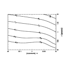
Figure 4: Rotation of M15 obtained with a thin-plate smoothing spline. The r and z axis are perpendicular and along the rotation axis (220^∘) of the cluster, respectively. The contours are in $\rm{km}~{}\rm s^{-1}$.

To get a higher S/N estimate of the two-dimensional velocity structure we will assume axisymmetry. This assumption is invalid if the PA twists. However, we will regard the possible twisting in Fig. 3 as a perturbation to the global velocity structure and use the PA measured for the whole sample as the symmetry axis. We can then reflect stellar positions about both the rotation axis and a line perpendicular to that axis and re-estimate the velocity map, a procedure that will effectively increase the number of data points by a factor of four. Figure 4 plots the resulting axisymmetric isovelocity contours in a single quadrant, calculated using the same smoothing spine as above. Here the y and x axes are along and perpendicular to the rotation axis, respectively.

The projected rotation of a spherical system with solid-body internal rotation (i.e., rotation velocity constant on cylinders) will have isovelocity contours parallel to the rotation axis. This is guaranteed because, along the line-of-sight at a fixed projected distance from the axis, the linear decrease in the radial velocity due to the changing projection of the rotation on the line-of-sight is offset by the linear increase in the internal solid-body rotation profile. The vertical contours of Fig. 4 suggest that the rotation in M15 is consistent with an internal solid-body rotation profile. A similar non-parametric estimate of the symmetrized rotation map for 47 Tuc shows the rotation decreasing below that expected for a solid-body form beyond a radius of 2′ (Paper 2). The half-light radius of M15 is 2.9$\times$ smaller than that of 47 Tuc (Trager et al. 1993; primarily reflecting the larger distance of M15), so the two clusters may have real differences in the form of their rotation. More velocities are need at large radii in M15 to be sure of this, however.

Figure 3 suggests that the rotation PA changes from north-south at small radii to more east-west at large. We can check the significance of this result by radially binning the individual stars and estimating the rotation properties in each bin. We use a maximum likelihood estimator that yields the amplitude and phase for a sinusoidal variation of the mean velocity with position angle, and the dispersion around the sinusoid, while holding the mean velocity of the sample fixed at the cluster mean. The results are given in Table 3 and plotted in Fig. 5. The solid points in the two panels of Fig. 5 are the rotation amplitude and position angle as a function of radius for five bins containing 300 stars and a final outer bin of 74 stars. The amplitude of the rotation from Fig. 5 will not match that of Fig. 4 since, unlike Fig. 5, Fig. 4 is derived under the assumption of axisymmetry. The position angle of the rotation does increase beyond a radius of 1′, consistent with the twisting of the isovelocity contours in Fig. 3. However, this result depends somewhat on the binning adopted and more velocities at large radii are needed to confirm this feature.

The two innermost solid points in Fig. 5 suggest that the position angle of the rotation also changes at small radii, though the rotation amplitude of even the larger innermost point is small enough that it could occur by chance about 13% of the time. This feature might not appear as a twisting of the contours in Fig. 3 because of the smoothing.

To obtain a more detailed picture of the rotation profile at small radii, we turn to the procedure of using the integrated light developed in Paper 1. The Fabry-Perot observations provide two-dimensional images that yield an integrated-light spectrum at every sufficiently bright pixel and, hence, the two-dimensional velocity structure of the cluster. The integrated light provides a better estimate of the rotation properties than the individual velocities because it effectively samples a larger number of stars, which will limit the noise due to the cluster dispersion. We azimuthally bin and average velocities from the integrated-light velocity map and find the best-fit sinusoid. These results are also listed in Table 3 and plotted as open circles in Fig. 5. The results from the 1994 and 1995 CFHT data are similar and we show only the latter since the seeing was better in 1995.

The integrated light map only has adequate S/N within 20″ of the center; beyond that, we have to rely on the stellar velocities to determine the rotation properties. In the region where there is significant overlap, the rotation properties measured by the integrated light and the stars agree in both amplitude and position angle. The integrated-light results presented here are reasonably consistent with the corresponding results from Paper 1 for the region within a radius of 15″ (with a mean radius of 8″), which were an amplitude of $1.7\pm 0.3$ $\rm{km}~{}\rm s^{-1}$ and a position angle for the maximum positive rotation velocity of $220\arcdeg\pm 11\arcdeg$. Our new results support a change in the position angle of the rotation axis at small radii and suggest that the rotation amplitude increases as well.

However, in the central regions, seeing and sampling noise become an important consideration for interpreting the integrated-light rotation properties. Peterson (1993) reported a streaming motion with a full range of 15 $\rm{km}~{}\rm s^{-1}$ in the central 1″ of M15. Dubath & Meylan (1995), using CORAVEL with slits at various positions in the center of M15, argued that Peterson’s result may have been due to sampling noise. The two brightest stars in the central region (AC212 and AC215) have velocities differing by 30 $\rm{km}~{}\rm s^{-1}$ and are aligned along the direction for which the streaming motion was reported. Using our two-dimensional velocity map, we find a result similar to that of Dubath & Meylan. By synthesizing the slit position and size of Peterson’s observation, our velocity map shows the same change in the mean velocity with position as Peterson measured; however, the result is due to contamination from the wings of the two bright stars, emphasizing the importance of understanding the sampling noise (Dubath 1993). Our integrated-light rotation measurements will suffer from the same problem. For seeing of 0.8″, we estimate that the radius at which two stars may cause a rotation signature is around 2″. The vertical dashed line in Fig. 5 is at this radius. However, the PA changes smoothly from larger radii to the smallest radius, giving us confidence that the increase in the rotation amplitude at small radii seen in Fig. 5 is a physical effect, and not due to sampling.

We can further check the significance of the central increase in the rotation by exploiting the two-dimensional data of the FP. We subtract the five brightest stars in the central 4″, re-calculate the velocity map, and estimate the rotation from the map as before. This procedure may show the influence of the bright stars on the inferred central rotation. The rotation obtained in this way does not show the characteristics seen in Fig. 5; in fact, there is no detectable rotation when the five bright stars are subtracted. However, this result may be due mainly to noise in the subtraction. Inspection of the line profiles for the integrated light before and after subtraction demonstrates that the subtraction added significant noise, making determination of the line centroid uncertain. Another method, instead of subtracting the bright stars, is to ignore the pixels out to some radius underlying those stars. This procedure gives similar results to those in Fig. 5, but it is questionable since it depends on the radius chosen. Yet another check is to measure the rotation from the stellar velocities inside of 2″. For the 12 stars inside of 2″, we measure a rotation amplitude of $8.5\pm 3.8$ $\rm{km}~{}\rm s^{-1}$ and a PA of $303$^∘$\pm 26$, consistent with the integrated light profile. We conclude that the rotation inside of 2″ appears significant. However, better-seeing data are needed to reduce the sampling uncertainties and we, therefore, have chosen a radius of 2″ as the boundary inside of which our results may have been affected by this.

3.3 Velocity Dispersion

Fig. 6 plots for our M15 sample the absolute magnitude of the deviation of each stellar velocity from the cluster mean velocity vs. radius. The points are the velocity measurements, and the solid and dashed lines are the LOWESS estimates of both the velocity dispersion and the 90% confidence band, respectively (see Paper 2 for details). The dispersion does not increase significantly inside a radius of 0.4′.

This dispersion profile is consistent not only with that of Paper 1 but also, outside of a radius of 1″, with the profile increasing towards smaller radii which was found by PSC. However, in the central 1″, PSC reported a cusp in the velocity dispersion based on integrated-light measurements. Our larger sample, which has four stars within 1″ of the center, shows no evidence for a central cusp. PSC’s high velocity dispersion measurement may have been due to sampling noise (Dubath 1993, Zaggia et al. 1993). Our estimate of the dispersion uses a smoothing length, which prevents our estimated profile from changing quickly. However, the dispersion of the four stars in the central 1″ is 11.6 $\rm{km}~{}\rm s^{-1}$, consistent with the LOWESS estimate of Fig. 6; this estimate is also consistent with the results of Dubath & Meylan (1994) and Dull et al. (1996).

4 MASS MODELING

4.1 Non-Parametric Estimate

We have used the non-parametric mass modeling technique of GF to estimate the mass density profile for M15. Under the assumptions of spherical symmetry and an isotropic distribution of velocities at all points, the Abel equations provide estimates of the deprojected luminosity density and velocity dispersion profiles, given the projected quantities. With the same assumptions, the Jeans equation then yields a unique mass density profile. We use the velocity dispersion profiles from Fig. 6, and the surface brightness profiles from Grabhorn et al. (1992) and Guhathakurta et al. (1996). Figure 7 plots the resulting non-parametric estimates of the mass density and the mass-to-light ratio (M/L) profiles. The solid lines are the bias-corrected estimates and the dotted lines are the 90% confidence bands. The bias is estimated through bootstrap resamplings (see GF).

The dashed line in the upper panel of Fig. 7 has a slope of –2.23, which is the theoretical prediction for the region outside of the core in a core-collapse cluster (Cohn 1980). Theory and observation are clearly in good agreement. Fig. 8 plots the logarithmic slope of the mass density profile and its 90% confidence band. Since derivatives are inherently noisier, the uncertainties on the slope are large; particularly at large radii the slope is highly uncertain. Not that the confidence bands depend on the amount of smoothing which has been introduced in the velocity dispersion estimate. Also, the uncertainties in the surface brightness profile are not considered here and may significantly increase the uncertainties in the slope estimate. The confidence band shown in Fig. 8 only reflects the uncertainty based on the smoothing used for Fig. 7; a more rigorous treatment would have to include the surface brightness uncertainties and try different velocity dispersion smoothings.

Phinney (1992, 1993) used measurements of pulsar accelerations to estimate the central density in M15 and found a value of greater than $2\times 10^{6}~{}{\rm M}_{\odot}$/pc³. We are able to follow M15’s mass density over five decades of density (two of radius). In the central 1.4″ (0.07 parsecs) the inferred density reaches $2\times 10^{6}~{}{\rm M}_{\odot}$/pc³ with 1$\sigma$ uncertainties under 30%, in concordance with Phinney’s value.

The estimated M/L_V for M15 increases from about 1.2 at a radius of 10″ (0.5 pc) to nearly 3 in the central 0.05 parsecs. There is a similar, but more statistically significant, increase in the outer 8 parsecs. We attribute these increases to a concentration of heavy stellar remnants in the central regions and of low-mass stars in the outer parts.

Rotation has not been included in this analysis. However, the dispersion about the average rotation velocity of 2.0 $\rm{km}~{}\rm s^{-1}$ for our M15 sample is 9.8 $\rm{km}~{}\rm s^{-1}$. The ratio of the squares of these quantities, which measures the dynamical significance of rotation, is 0.04. In regions where the rotation velocity is as large as 4 $\rm{km}~{}\rm s^{-1}$(see Fig. 5), this ratio approaches 0.2. Still, our dispersion values in Fig. 6 were increased by ignoring the rotation, which approximately mimics the effect of rotation in the Jeans equations, so our mass distribution calculated without including rotation will likely be a good approximation.

GF also presented a mass density profile for M15 and their profile differs from the one presented here. In GF, there was a shoulder in the mass density profile at a radius of 2.0 parsecs (about 0.8′), which is not present in Fig. 7. The main reason for the difference is the increase in the size of our velocity sample by a factor of two, which obviously reduces the noise in our estimation. A related effect is the increased radial coverage of the CFHT data, which spans more than two decades compared to one for the CTIO data in GF. This larger coverage makes it easier to distinguish noise from trends and so choose a realistic smoothing. This choice presents more of a problem with non-parametric techniques that impose smoothing on the projected quantities, as we do here, rather than ones that impose smoothing in the space of the desired function (see Merritt & Tremblay 1994), since the noise in the projected quantities will be amplified upon deprojection. We feel that the mass density profile for M15 in GF may have been undersmoothed.

4.2 Black Hole Models

We can also invert the above procedure by assuming a mass density profile for M15 and calculating the projected velocity dispersion implied by the isotropic Jeans equation. Figure 9 shows the projected dispersion profiles that result from assuming that M15 has a uniform stellar M/L and a central black hole with various values for the mass. The dashed and dotted lines are the estimated velocity dispersion profile and the 90% confidence band from Fig 6. The solid lines are the expected velocity dispersion profiles assuming a stellar M/L of 1.7 and black hole masses of 0, 500, 1000, 3000, and 6000 ${\rm M}_{\odot}$. Note that all of these models with an M/L that does not change with radius are just excluded at 90% confidence because they rise too steeply between a radius of 100″ and 10″. We will discuss the possibility of a black hole at the center of M15 in § 5.

4.3 Mass Functions

We can estimate the present-day mass function of M15 using the technique described in GF. The Jeans equation relates the cluster potential and the number density and velocity dispersion profiles of a tracer population. We calculate the cluster potential from the mass density determined in § 4.1. If we know the velocity dispersion profile for some population, then we can calculate the number density profile for that population up to a multiplicative constant. As in GF, we will assume local thermodynamic equilibrium (LTE); LTE allows us to relate the observed dispersion profile of the giants and turnoff stars to the profiles of objects with other masses. This method will only yield an approximate result, since LTE is not strictly valid at any radius and is, moreover, a poor approximation for low-mass objects at large radii. The mass density profiles for the individual mass components must sum to the total density profile. We determine the necessary multipliers for each number density profile using maximum penalized likelihood. To keep the derived mass function reasonably smooth, we use the second derivative of the mass function as the penalty function (equations 7–9 of GF).

Figure 10 plots the resulting mass functions for M15. The different lines represent different radial ranges and their 68% confidence bands: the solid lines are the mass function for the inner 25% of the mass (0.0–2.0 pc); the dashed lines that for the 25–50% mass range (2.0–5.0 pc); and the dotted lines that for the 50–75% mass range (5.0–8 pc). The solid points are located at the masses used in the fitting.

Both luminous and non-luminous objects contribute to the mass functions in Fig. 10. The global cluster M/L provides a constraint on the relative contributions, but exploiting this requires knowing the uncertain light-to-mass ratios (L/M) for the main-sequence and giant stars in the various mass groups. We begin by calculating the cluster M/L assuming that all of the stars with masses below the turn-off are luminous. Multiplying the L/M’s of the various mass groups by the mass function yields the total cluster luminosity, which we may then divide into the dynamically-estimated total cluster mass. The L/M values that we used are based on direct estimates from color-magnitude diagrams (see Pryor et al. 1991). The values are (m is the stellar mass in solar units) zero for m$<0.16$ and m$>0.8$, 0.014 for $0.16<{\rm m}<0.25$, 0.026 for $0.25<{\rm m}<0.40$, 0.14 for $0.40<{\rm m}<0.63$, 4.6 for $0.6<{\rm m}<0.8$ (including giant stars). The ratio of this population M/L to the average dynamical M/L derived from the normalization of the velocity dispersion profile is approximately the fractional contribution of the main-sequence and giants stars to the total mass. The M/L derived from the velocity dispersion normalization is 1.7 (§4.2), and the M/L derived from the mass function is 0.3. The ratio implies that 85% of mass is in non-luminous objects not included in the L/M values, presumably stellar remnants.

The mass functions in Fig. 10 argue that much of the mass of M15 is in the form of 0.6–0.7 ${\rm M}_{\odot}$ objects, presumably white dwarfs. GF reached the same conclusion for M15 and three other clusters. This result may be in conflict with the mass of 0.5 ${\rm M}_{\odot}$ found by Richer et al. (1995) for white dwarfs in the globular cluster M4 based on their location in the color-magnitude diagram. However, some heavier white dwarfs are also expected from the evolution of massive main-sequence stars early in the history of the cluster.

The constraints on the numbers of lower-mass objects ($<$ 0.3 M_⊙) are not as firm due to the uncertainty in the velocity dispersion at large radii, as reflected in the larger confidence band, and due to the assumption of LTE. A more reasonable approach would be to estimate properly the relation between the velocity dispersion profiles for different masses using Fokker-Planck simulations. However, we find relatively few objects with masses below $0.3~{}{\rm M}_{\odot}$. This last result contradicts GF, who found mass functions increasing at the smallest masses for all of the clusters that they studied, including M15. The different result yielded by the larger velocity dataset presented here demonstrates the sensitivity of the mass function estimate to noise in the data.

5 SUMMARY AND DISCUSSION

Knowledge of the present-day stellar mass function in globular clusters is crucial for understanding the initial mass function. The latter contains important information about star formation in the early galaxy and plays an important role in cluster dynamical evolution (e.g., Angelletti & Giannone 1979; Chernoff & Weinberg 1990). Dull et al. (1996) have produced an extensive set of Fokker-Planck models for M15 and find that the projected dispersion profile is well fitted by a post-collapse model. From this model, they estimate that there are a few $\times$ $10^{4}$ objects more massive than 1 ${\rm M}_{\odot}$ in the central 6″ (0.3 pc). Integrating our estimated mass function (Fig. 10) over objects more massive than 1 ${\rm M}_{\odot}$ gives about 2000 objects, which are all in the innermost 25% of the mass (radii smaller than 2.0 pc). Both models find a few $\times$ $10^{5}$ objects with masses of about 0.7 ${\rm M}_{\odot}$, which are presumably a combination of main-sequence stars and stellar remnants (white dwarfs). The largest disagreement between their and our mass function is for the numbers of low-mass objects. Dull et al. find a few $\times 10^{5}$ stars with masses less than 0.3${\rm M}_{\odot}$, which is higher than our 95% confidence level for these masses.

It needs to be stressed that both of the above dynamical estimates of the present-day mass function are uncertain: our results will be inherently noisy since we are trying to estimate the quantities directly from the data, while Dull et al. require assumptions about the initial mass function and the relation between the initial stellar mass and the final remnant mass, both of which may have large uncertainties. The strongest conclusions about the M15 mass function are those found by both: that a large number (2000 to $10^{4}$) of 1.4 ${\rm M}_{\odot}$ objects are present in the central region and that most of the cluster mass is in 0.5-0.7 ${\rm M}_{\odot}$ objects. These conclusions can be compared to those of Heggie & Hut (1996), who find that approximately 50% of 47 Tuc’s mass may be in the form of white dwarfs or lower-mass stars. Our results suggest that white dwarfs, rather than lower-mass stars, constitute most (about 85%) of the mass of M15.

Strengthening our dynamical estimates of M15’s mass function requires larger number of velocities in the outer regions ($R>2$′) of M15. Low-mass stars are expected to populate the regions at large radii, where photometric studies have shown that there may be significant numbers of low-mass stars (Hesser et al. 1987, Richer et al. 1990). Since photometric estimates of the number of low-mass stars require large completeness corrections and depend on the uncertain main-sequence mass-luminosity relation, dynamical estimates provide valuable additional constraints.

The theory of core collapse appears to pass a very basic test: the mass density profile for M15 shown in Fig. 7 is remarkably well fit by a power law with an index of –2.2 throughout most of its radial extent, as predicted (Cohn 1980). There is a shallow “shoulder” in the profile at a radius of about 0.2′ which is suggestive of a transition between most of the density being provided by massive stellar remnants and most by stars with the turnoff mass (the latter having a shallower profile). Unfortunately, Dull et al. (1996) did not show the spatial density profiles of their Fokker-Planck models. The projected density profiles (their Fig. 10) do suggest that this transition should occur at about that radius. However, our measured projected velocity dispersion profile in Fig. 9 is somewhat flatter than the profiles predicted by the the Dull et al. models (see their Fig. 6), which increase from a value of 9.5 $\rm{km}~{}\rm s^{-1}$ at 30″ to 12 $\rm{km}~{}\rm s^{-1}$ at 3″.

Rotation has generally not been included in calculations of globular cluster evolution and we stress the importance doing so in light of our results for M15. The radial profiles of the rotation PA and amplitude, such as are shown in Fig. 5, could provide significant constraints for such models. Recently, Einsel & Spurzem (1996) have produced Fokker-Planck simulations including rotation. Their projected rotation curve is similar to what we measure using the stellar velocities, presented as the solid points in Fig. 5: there is a peak in the rotation amplitude close to the half-mass radius. Unfortunately, we have too few velocities at large radii to allow a detailed comparison there to the results of Einsel & Spurzem. Unlike the broad agreement at larger radii, in the central region we find a possible increase in the rotation amplitude which is not seen in their results. One explanation could be the existence of a central mass concentration not included in the models. Since the models contain only a single-mass stellar component, possibilities are both heavy remnants and a massive central black hole. We also see a large change in the rotation position angle at small radii, which is even harder to understand theoretically. Both the theory and the data need to be improved for the region near the center of the cluster.

Fig. 9 suggests that the maximum allowed black hole mass is around 3000 ${\rm M}_{\odot}$. However, this number is uncertain due to our assumptions of isotropy and constant M/L. Fully 2-integral, and possibly 3-integral, models are necessary to adequately constrain the maximum allowed black hole mass from the velocity dispersion data alone.

Whether or not M15 contains a central black hole remains open. Fig. 9 suggests that the best isotropic model with a constant stellar M/L is one that contains a black hole of 1000 ${\rm M}_{\odot}$. However, if the M/L is allowed to vary, then the velocity dispersion data imply a change from 1.7 at large radii to only 3 in the central region (Fig. 7). This barely significant change could be caused by only the modest number of heavy-remnants predicted in the central region of old globular clusters by Fokker-Planck simulations such as those of Dull et al. (1996). Both models – a 1000 ${\rm M}_{\odot}$ central black hole and an increase of the M/L to 3 – have the same projected velocity dispersion profile. Thus, even with additional velocity data in the central regions, it will be difficult to discriminate between them. One alternative is to use the rotation properties to discriminate between the models. For instance, a central mass concentration could cause an increase in the rotation amplitude at smaller radii, as has been observed in Fig. 5. Determining the strength of such a test will require detailed modeling including a central mass concentration and more sophisticated Fokker-Planck simulations.

In summary, even excellent ground-based seeing ($\sim 0.8\arcsec$) still imposes significant uncertainties on the rotation and velocity dispersion profiles of M15 at small radii. Better data would reduce the present uncertainties in these profiles in the central region and might reveal behavior that cannot be produced by the change in M/L resulting from mass segregation. For example, the velocity dispersion produced by a 3000 ${\rm M}_{\odot}$ central black hole would lead to an increase of the inferred M/L to around 8 at a radius of 0.03 pc, which would be difficult to obtain with any reasonable remnant population. The data to test such predictions will require adaptive optics or HST.

Figure 1: Comparison of the Fabry-Perot velocities for stars in M15 with the Fabry-Perot velocities of Paper 1.

Figure 2: Radial velocities plotted vs. radius from the center of M15. The solid horizontal line is at the sample mean of $-107.8\pm 0.3$ $\rm{km}~{}\rm s^{-1}$.

Figure 5: Rotation position angle and amplitude as a function of radius. The solid points come from the best fit sinusoid to the individual velocities in radial bins of 300 stars. The open circles are the best-fit parameters for the azimuthally binned and averaged velocities from the integrated-light velocity map. The dashed line is the estimate of the radius (2″) where seeing may significantly affect the estimate of the rotation from the integrated light.

Figure 6: Velocity dispersion of M15. The points are the absolute deviations of the individual velocity measurements from the cluster mean velocity ($-107.8\pm 0.3$ $\rm{km}~{}\rm s^{-1}$). The solid line represents the LOWESS estimate of the velocity dispersion, and the dashed lines are the 90% confidence band. For M15, 1′ is 2.8 parsecs.

Figure 7: Mass density and M/L ratio profile for M15. The solid lines are the non-parametric estimates and the dotted lines are the 90% confidence bands. The dashed line in the upper figure is a power-law slope of –2.23.

Figure 8: Logarithmic slope of the mass density as a function of radius. The solid and the dashed lines are the slope and the 90% confidence bands, respectively. The dotted line is at the value –2.23.

Figure 9: The dashed and dotted lines are the estimate of the velocity dispersion and its 90% confidence band as a function of radius, respectively. The solid lines are the projected velocity dispersion assuming constant M/L=1.7, isotropy, and central black hole masses of 0, 100, 1000, 3000, and 6000 ${\rm M}_{\odot}$.

Figure 10: Mass function for M15. The heavy and light solid lines represent the values for the inner 25% mass and its 90% confidence band, respectively. The heavy dashed and dotted lines are for the second and third quartiles of the mass, respectively, and the corresponding light lines are their confidence bands.

References

- (1)
- (2) Angelleti, L., & Giannone, P. 1979, A&A, 85, 113
- (3) Armandroff, T. E., Olszewski, E. W., & Pryor, C. 1995, AJ, 110, 2131
- (4) Bates, D., Lindstrom, M.J., Wahba, G., & Yandell, B.S. 1986, Technical Report No. 775, Univ. of Wisconsin
- (5) Chernoff, D. F., & Weinberg, M. D. 1990, ApJ, 351, 121
- (6) Clevelend, W., & McGill, R. 1984, J.Am.Stat.Assoc., 79, 807
- (7) Cohn, H. 1980, ApJ, 242, 765
- (8) Craven, P., & Wahba, G. 1979, Numer. Math., 31, 377
- (9) Dubath, P. 1993, Ph.D. thesis, University of Geneva
- (10) Dubath, P., Meylan, G., & Mayor M. 1995, ApJ, 426, 192
- (11) Duquennoy, A., & Mayor, M. 1991, A&A, 248, 485
- (12) Dull, J.D. et al. 1996, ApJ, in press
- (13) Einsel, C. & Spurzem, R. 1996, preprint
- (14) Gebhardt, K., & Fischer, P. 1995, AJ, 109, 209 (GF)
- (15) Gebhardt, K., Pryor, C., Williams, T.B., Hesser, J.E. 1994, AJ, 107, 2067 (Paper 1)
- (16) Gebhardt, K., Pryor, C., Williams, T.B., Hesser, J.E. 1995, AJ, 110, 1699 (Paper 2)
- (17) Gebhardt, K., Richstone, D. et al. 1996, AJ, 112, 105
- (18) Grabhorn, R. P., Cohn, H. N., Lugger, P. M., & Murphy, B. W. 1992, ApJ, 392, 86
- (19) Guhathakurta, P., Yanny, B., Schneider, D., & Bachall, J. 1996, AJ, 111, 267
- (20) Gunn, J.E. & Griffin, R. F. 1979, AJ, 84, 752
- (21) Heggie, D., & Hut, P. 1996, preprint
- (22) Hesser, J.E., Harris, W.E., VandenBerg, D.A., Allwright, J.W.B., Shott, P., & Stetson, P. 1987, PASP, 99, 739
- (23) Latham, D. W., & Stefanik, R. P. 1992, IAU Transactions Vol. XXIB, edited by J. Bergeron, (Kluwer: Dordrecht), p. 269
- (24) Lauer, T., Holtzman, J., Faber, S., et al. 1991, ApJ, 369, L45
- (25) Le Fevre, O., Crampton, D., Felenbok, P., Monnet, G. 1994, å, 282, 325
- (26) Lupton, R.H., Gunn, J.E., & Griffin, R.F. 1987, AJ, 93, 1114
- (27) Makino, J., & Aarseth, S.J. 1992, PASJ, 44, 141
- (28) Mayor, M. et al. 1983, A&AS, 54, 495
- (29) McMillan, S., & Aarseth, S.J. 1993, ApJ, 414, 200
- (30) Merritt, D. 1993a, in Structure and Dynamics of Globular Clusters, edited by S.G. Djorgovski, & G. Meylan, (Astronomical Society of the Pacific), p. 117
- (31) Merritt, D. 1993b, in Structure, Dynamics and Chemical Evolution of Elliptical Galaxies, ed. I.J. Danziger, W.W. Zeilinger & K. Kjär (ESO, Munich), p. 275
- (32) Merritt, D., & Tremblay, B. 1994, AJ, 108, 514
- (33) Meylan, G., Dubath, P., & Mayor, M. 1991, ApJ, 383, 587
- (34) Morbey, C. 1992, Applied Optics, 31, 2291
- (35) Peterson, R.C. 1993, in Structure and Dynamics of Globular Clusters, edited by S.G. Djorgovski, & G. Meylan, (Astronomical Society of the Pacific), p. 65
- (36) Peterson, R.C., Seitzer, P., & Cudworth, K.M. 1989, ApJ, 347, 251 (PSC)
- (37) Phinney, E.S. 1992, Phil.Trans.R.Soc.Lond. A, 341, 39
- (38) Phinney, E.S. 1993, in Structure and Dynamics of Globular Clusters, edited by S.G. Djorgovski, & G. Meylan, (Astronomical Society of the Pacific), p. 141
- (39) Pryor, C., McClure, R.D., FLetcher, J.M., & Hesser, J.E. 1991, AJ, 102, 1026
- (40) Richer, H.B., Fahlman, G.C., Buonanno, R. & Fusi Pecci, F. 1990, ApJ, 359, L11
- (41) Richer, H.B., et al. 1995, ApJ, 451, L17
- (42) Stetson, P.B. 1994, PASP, 106,250
- (43) Wahba, G. 1980, Technical Report No. 595, Univ. of Wisconsin
- (44) Wahba, G. 1990, Spline Models for Observational Data, (Soc. for Industrial and Applied Mathematics: Philadelphia)
- (45) Zaggia, S.R., Capaccioli, M., & Piotto, G. 1993, A&A, 278, 415
- (46)