ON THE FRACTAL STRUCTURE OF THE VISIBLE UNIVERSE

Abstract

Some years ago we proposed a new approach for the analysis of galaxy and cluster correlations based on the concepts and methods of modern Statistical Physics. This led to the surprising result that galaxy correlations are fractal and not homogeneous up to the limits of the available catalogues. In the meantime many more redshifts have been measured and we have extended our methods also to the analysis of number counts and angular catalogues. This has led to a complete analysis of all the available data that we are going to present in detail in this lecture. In particular we will discuss the properties of the following catalogues: CfA, Perseus-Pisces, SSRS, IRAS, Stromlo-APM, LEDA, Las Campanas and ESP for galaxies and Abell and ACO for clusters. The result is that galaxy structures are highly irregular and self-similar. The usual statistical methods, based on the assumption of homogeneity, are therefore inconsistent for all the length scales probed until now. A new, more general, conceptual framework is necessary to identify the real physical properties of these structures. In the range of self-similarity theories should shift from ”amplitudes” to ”exponents”. The new analysis shows that all the available data are consistent with each other and show fractal correlations (with dimension $D\simeq 2$) up to the deepest scales probed until now ($1000h^{-1}Mpc$) and even more as indicated from the new interpretation of the number counts. The distribution of visible matter in the universe is therefore fractal and not homogeneous. The evidence for this being very strong up to $150h^{-1}Mpc$ due to the statistical robustness of the data and progressively weaker (statistically) at larger distances due to the limited data. In addition the luminosity distribution is correlated with the space distribution in a specific way characterized by multifractal properties. These facts lead to fascinating conceptual implications about our knowledge of the universe and to a new scenario for the theoretical challenge in this field.

1 Introduction

This lecture reports the evidences for the fractal properties of visible matter in the universe in relation to the debate with Prof. M. Davis. We have also included new elements stimulated by the debate, like the analysis of the Stromlo-APM galaxy catalogue and a discussion of the angular data. For a comprehensive and detailed report the reader may refer to [1] and to a more recent review [2].

From the experimental point of view there are four main facts in Cosmology: - The space distribution of galaxies and clusters: the recent availability of several three dimensional samples of galaxies and clusters permits the direct characterization of their correlation properties. - The cosmic microwave background radiation (CMBR), that shows an extraordinary isotropy and an almost perfect black body spectrum. - The linearity of the redshift-distance relation, usually known as the Hubble law. This law has been established by measuring independently the redshift and the distance of galaxies. - The abundance of light elements in the universe. Each of these four points provides an independent experimental fact. The objective of a theory should be to provide a coherent explanation of all these facts together.

Our work refers mainly to the first point, the space distribution of galaxies and clusters which, however, is closely related to the interpretation of all the other points. In particular we claim that the usual methods of analysis are intrinsically inconsistent with respect to the properties of these samples. The correct statistical analysis of the experimental data, performed with the methods of modern Statistical Physics, shows that the distribution of galaxies is fractal up to the deepest observed scales [4] [1]. This result has caused a strong debate in the field because it is in contrast with the usual assumption of large scale homogeneity which is at the basis of most theories. Actually homogeneity represents much more than a working hypothesis for theory, it is often considered as a paradigm or principle and for some authors it is conceptually absurd even to question it [5]. For other authors instead homogeneity is just the simplest working hypothesis and the idea that nature might actually be more complex is considered as extremely interesting [6]. These two points of view are not so different after all because, if something considered absurd becomes real, then it is indeed very exciting. Given this situation it may be interesting to analyze why this question develops such strong feelings. This will help us to distinguish opinions from bare facts and to place the discussion in the appropriate perspective.

Figure 1: Example of analytical and nonanalytic structures. Top panels (Left) A cluster in a homogenous distribution. (Right) Density profile. In this case the fluctuation corresponds to an enhancement of a factor 3 with respect to the average density. Bottom panels (Left) Fractal distribution in the two dimensional Euclidean space. (Right) Density profile. In this case the fluctuations are non-analytical and there is no reference value, i.e. the average density. The average density scales as a power law from any occupied point of the structure.

Most of theoretical Physics is based on analytical functions and differential equations. This implies that structures should be essentially smooth and irregularities are treated as single fluctuations or isolated singularities. The study of critical phenomena and the development of the Renormalization Group (RG) theory in the seventies was therefore a major breakthrough [7] [8]. One could observe and describe phenomena in which intrinsic self-similar irregularities develop at all scales and fluctuations cannot be described in terms of analytical functions. The theoretical methods to describe this situation could not be based on ordinary differential equations because self-similarity implies the absence of analyticity and the familiar mathematical Physics becomes inapplicable. In some sense the RG corresponds to the search of a space in which the problem becomes again analytical. This is the space of scale transformations but not the real space in which fluctuations are extremely irregular. For a while this peculiar situation seemed to be restricted to the specific critical point corresponding to the competition between order and disorder. In the past years instead, the development of Fractal Geometry [9], has allowed us to realize that a large variety of structures in nature are intrinsically irregular and self-similar (Fig.1).

Mathematically this situation corresponds to the fact that these structures are singular in every point. This property can be now characterized in a quantitative mathematical way by the fractal dimension and other suitable concepts. However, given these subtle properties, it is clear that making a theory for the physical origin of these structures is going to be a rather challenging task. This is actually the objective of the present activity in the field [10]. The main difference between the popular fractals like coastlines, mountains, trees, clouds, lightnings etc. and the self-similarity of critical phenomena is that criticality at phase transitions occurs only with an extremely accurate fine tuning of the critical parameters involved. In the more familiar structures observed in nature instead the fractal properties are self-organized, they develop spontaneously from the dynamical process. It is probably in view of this important difference that the two fields of critical phenomena and Fractal Geometry have proceeded somewhat independently, at least at the beginning.

The fact that we are traditionally accustomed to think in terms of analytical structures has crucial consequences on the type of questions we ask and on the methods we use to answer them. If one has never been exposed to the subtleness on nonanalytic structures, it is natural that analyticity is not even questioned. It is only after the above developments that we could realize that the property of analyticity can be tested experimentally and that it may or may not be present in a given physical system.

We can now appreciate how this discussion is directly relevant to Cosmology by considering the question of the Cosmological Principle (CP). It is quite reasonable to assume that we are not in a very special point of the universe and to consider this as a principle, the CP. The usual mathematical implication of this principle is that the universe must be homogeneous. This reasoning implies the hidden assumption of analyticity that often is not even mentioned. In fact the above reasonable requirement only leads to local isotropy. For an analytical structure this also implies homogeneity [6]. However, if the structure is not analytical, the above reasoning does not hold. For example a fractal structure has local isotropy but not homogeneity. In simple terms one observes the same mix of structures and voids in different directions (statistical isotropy). This means that a fractal structure satisfies the CP in the sense that all the points are essentially equivalent (no center or special points) but this does not imply that these points are distributed uniformly. In this respect the saturation of the dipole moment cannot be considered as a test of homogeneity because this property is also present in fractal structures [11].

This important distinction between isotropy and homogeneity has not been adequately appreciated in M. Davis’ lecture, and it has other important consequences. For example it clarifies that drawing conclusions about real galaxy correlations from the angular distributions alone can be rather misleading as we are going to see in detail later. In addition, from this new perspective, the isotropy of the CMBR may appear less problematic in relation to the highly irregular three dimensional distribution of matter and this may lead to theoretical approaches of novel type for this problem. In the present work, however, we are going to limit our discussion to the optimal way to analyze the data provided by the galaxy catalogues from the broader perspective in which analyticity and homogeneity are not assumed a priori but they are explicitly tested. The main result is that the data become actually consistent with each other and coherently point to the same conclusion of fractal correlations up to the present observational limits. In this lecture we present a colloquial discussion of the main results and their implications.

2 Statistical Methods and Correlation Properties

- Usual arguments: Before the extensive redshift measurements of the 80s the information about the galaxy distribution was only in terms of the two angular coordinates. These angular distributions appeared rather smooth at relatively large angular scale, like for example the lower part of Fig.2.

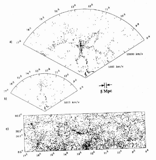
Figure 2: A slice of the three dimensional galaxy distribution (a) (b) compared with the corresponding (c) angular distribution (the portion between $26.5^{\circ}$ and $32.5^{\circ}$ - [11]). Note that the angular distribution appears relatively homogenous while the real three distribution in space is much more irregular. In particular this picture shows the so-called Great Wall which extends over the entire sample (at least $170h^{-1}Mpc$). Note that it is impossible to identify structures of this typo from the angular data alone. We also show the size of the galaxy ”correlation-length” ($r_{0}=5h^{-1}Mpc$) derived from the standard analysis. The more general analysis we discuss here implies instead that an eventual correlation length should be larger than any observable structure, i.e. $\gg 170h^{-1}Mpc$ and that the present data show well defined fractal properties up to the sample limits. These pictures clarify the intrinsic ambiguity of the angular catalogs in relation to the arguments of Prof. Davis. They show that a fractal distribution in 3-d (top) projects in a smooth angular distribution (bottom). No one could have predicted the real 3-d properties from the angular distribution alone.

Assuming that this smoothness corresponds to a real homogenization in 3-d space and estimating the characteristic depth of the angular catalogue from the magnitudes ”a characteristic length” $r_{0}=5h^{-1}Mpc$ has been estimated [5]. The idea was that beyond such a distance the 3-d galaxy distribution would become gradually homogeneous and it could be well approximated by a constant galaxy density. This average density, apart from the eventual Dark Matter, would be the one to use into Einstein equations to derive the Friedmann metric and the other usual concepts.

Later, the measurements of the galaxy redshifts plus the Hubble law provided also the absolute distances and could identify the position of galaxies in space. However the 3-d galaxy distributions turned out to be much more irregular with respect to their angular projections and showed large structures and large voids, as shown in the upper part of Fig.2. At first these irregular structures appeared to be in contradiction with the picture derived from the angular catalogues and, as we are going to see, they really are. However in 1983 a correlation analysis of the 3-d distribution (CfA1 catalog [14]) was performed by Davis and Peebles [13] and the result was again that the correlation length was $r_{0}=5h^{-1}Mpc$ as for the angular catalogues. This seemed to resolve the puzzle because it was interpreted as if a relatively small correlation length can be consistent with the observation of large structures. This value for $r_{0}$ has not been seriously questioned even after the observation of huge structures, like the galaxy wall, that extend up to $\sim 170h^{-1}Mpc$. Fig.2 is a clear example of the smoothing effect of angular projections, and it already gives a clear indication of the compatibility of a fractal structure in 3-d with a smoother projection.

The usual correlation analysis is performed by estimating at which distance ($r_{0}$) the density fluctuations are comparable to the average density in the sample ($\xi(r)=\langle n(0)n(r)\rangle/\langle n\rangle^{2}-1$; $\xi(r_{0})\equiv 1$). Now everybody agrees that there are fractal correlations at least at small scales. The important physical question is therefore to identify the distance $\lambda_{0}$ at which, possibly, the fractal distribution has a crossover into a homogeneous one. This would be the real correlation length beyond which the distribution can be approximated by an average density. The problem is therefore to understand the relation between $r_{0}$ and $\lambda_{0}$: are they the same or closely related or do they correspond to different properties? This is actually a subtle point with respect to the concepts discussed in the introduction. In fact, if the galaxy distribution becomes really homogeneous at a scale $\lambda_{0}$ within the sample in question, then the value of $r_{0}$ is related to the real correlation properties of the distribution and one has $r_{0}\simeq\lambda_{0}/2$. If, on the other hand, the fractal correlations extend up to the sample limits, then the resulting value of $r_{0}$ has nothing to do with the real properties of the galaxy distribution but it is fixed just by the size of the sample [1].

New Perspective: Given this situation of ambiguity with respect to the real meaning of $r_{0}$ it is clear that the usual correlation study in terms of the function $\xi(r)$ is not the appropriate method to clarify these basic questions. The essential problem is that, by using the function $\xi(r)$, one defines the amplitude of the density fluctuations by normalizing them to the average density of the sample in question. This implies that the observed density should be the real one and it should not depend on the given sample or on its size apart from Poisson fluctuations. However, if the distribution shows long range (fractal) correlations, this approach becomes meaningless. For example if one studies a fractal distribution with $\xi(r)$ a characteristic length $r_{0}$ will be identified, but this is clearly an artifact because the structure is characterized exactly by the absence of any defined length [1].

The appropriate analysis of pair correlations should therefore be performed using methods that can check homogeneity or fractal properties without assuming a priori either one. The simplest method to do this is to consider directly the conditional density $\Gamma(r)\sim\langle n(0)n(r)\rangle$ without comparing it to the average. There are several other methods that have been discussed elsewhere [1] [2]. This is not all however because one has also to be careful not to make hidden assumptions of homogeneity in the specific procedure to evaluate these correlations. For example, if a galaxy is close to the boundary of the sample, it is possible that the sphere of radius $r$ around it, where the conditional density is computed, may lie in part outside the sample boundary. In this case the usual procedure is to use weighting schemes of various types to include also these points in the statistics. In this way one implicitly assumes that the fraction of sphere contained in the sample is sufficient to estimate the properties of the full sphere. This implies that the properties of a small volume are assumed to be the same as for a larger volume (the full sphere). This is a hidden assumption of homogeneity that should be avoided by including only the properties of those points for which a surrounding sphere of radius $r$ is fully included in the sample. These procedures are fully standard in modern statistical mechanics and a detailed description can be found in [1]. This means that the statistical validity of a sample is limited to the radius of the largest sphere that can be contained in the sample. We call this distance $R_{s}$ and it should not be confused with the sample depth $R_{d}$, which can be in general much larger, depending on the survey geometry.

In 1988 we reanalyzed the CfA1 catalogue [15]. The result was that the catalogue has statistical validity up to $R_{s}=20h^{-1}Mpc$ and, up this length, it shows well defined fractal correlations. This shows therefore that the ”correlation length” $r_{0}=5h^{-1}Mpc$ derived by [13] was a spurious result due to an inappropriate method of analysis and it has nothing to do with the real correlation properties of the system. A similar analysis of the Abell cluster catalogue also showed fractal properties up to $R_{s}=80h^{-1}Mpc$ so that also the cluster ”correlation length” $r_{0}^{c}=25h^{-1}Mpc$ [16] should be considered as spurious. One consequence of these results was that the so called galaxy-cluster mismatch could be automatically eliminated by the appropriate analysis. Also other properties like $\delta N/N$, directly related to $r_{0}$, suffer from the same consistency problems because of the lack of a reference value [17]. This situation led to a rather controversial debate in the field. In the meantime many more data have became available and we have performed a complete analysis of all the data for galaxies and clusters. In the following we report the main results.

3 Analysis of the Galaxy Distributions

Here we discuss the correlation properties of the galaxy distributions in terms of volume limited catalogues [1] arising from most of the 50.000 redshift measurements that have been made to date. A first important result will be that the samples are statistically rather good and their properties are in agreement with each other. This gives a new perspective because, using the standard methods of analysis, the properties of different samples appear contradictory with each other and often this is considered to be a problem of the data (unfair samples) while, we show that this is due to the inappropriate methods of analysis. In addition essentially all the catalogues show well defined fractal correlations up to their limits and the fractal dimension is $D\simeq 2$. The few exceptions to this result will be discussed and interpreted in detail.

Table 1: The volume limited catalogues are characterized by the following parameters: - $R_{d}(h^{-1}Mpc)$ is the depth of the catalogue - $\Omega$ is the solid angle - $R_{s}(h^{-1}Mpc)$ is the radius of the largest sphere that can be contained in the catalogue volume. This gives the limit of statistical validity of the sample. - $r_{0}(h^{-1}Mpc)$ is the length at which $\xi(r)\equiv 1$. - $\lambda_{0}$ is the eventual real crossover to a homogeneous distribution that is actually never observed. The value of $r_{0}$ is the one obtained in the deepest sample. The CfA2 and SSRS2 data are not yet available. See Ref [13], [17]-[23] and [31] (distance are expressed in $h^{-1}Mpc$).

Sample	$\Omega$ ($sr$)	$R_{d}$	$R_{s}$	$r_{0}$	$D$	$\lambda_{0}$
CfA1	1.83	80	20	6	$1.7\pm 0.2$	$>80$
CfA2	1.23	130	30	10	2.0	$?$
PP	0.9	130	30	10	$2.0\pm 0.1$	$>130$
SSRS1	1.75	120	35	12	$2.0\pm 0.1$	$>120$
SSRS2	1.13	150	50	15	2.0	$?$
Stromlo-APM	1.3	100	30	10	$2.2\pm 0.1$	$>150$
LEDA	$4\pi$	300	150	45	$2.1\pm 0.2$	$>150$
LCRS	0.12	500	18	6	$1.8\pm 0.2$	$>500$
IRAS $1.2Jy$	$4\pi$	80	40	4.5	$2.0\pm 0.1$	$\simeq 25$
ESP	0.006	700	10	5	$1.9\pm 0.2$	$>800$

Figure 3: Full correlation for the various available redshift catalogues in the range of distances $0.1\div 1000h^{-1}Mpc$. A reference line with a slope $-1$ is also shown (i.e. fractal dimension $D=2$). Up to $\sim 150h^{-1}Mpc$ the density is computed by the full correlation analysis, while above $\sim 150h^{-1}Mpc$ it is computed through the radial density. For the full correlation the data of the various catalogues are normalized with the luminosity function and they match very well with each other [2]. This is an important test of the statistical validity and consistency of the various data. In the insert panel it is shown the schematic behavior of the radial density versus distance computed from the vertex (see text) [27]. The behaviour of the radial density allows us to extend the power law correlation up to $\sim 1000h^{-1}Mpc$. However a rescaling is necessary to match the radial density to the conditional density [2].

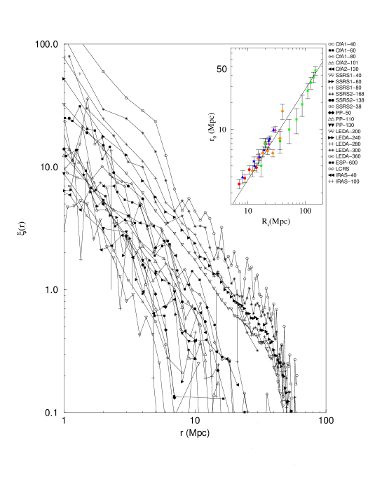
Figure 4: Usual analysis based on the function $\xi(r)$ of the same galaxy catalogues of Fig.3. This analysis is based on the a priori and untested assumption of the analyticity and homogeneity. These properties are not present in the real galaxy distributions and the results appear therefore rather confusing. This lead to the impression that galaxy catalogues are not good enough and to a variety of theoretical problems like the galaxy cluster mismatch, luminosity segregation, the linear and non linear evolution, etc.. The situation changes completely and it becomes rather clear if one adopts the more general framework that is at the basis of Fig.3. In the insert panel we show the dependence of $r_{0}$ on $R_{s}$ for all the catalogs. The linear behaviour is a consequence of the fractal nature of galaxy distribution in these samples [2].

The main data of our correlation analysis are collected in Fig.3 (left part) in which we report the conditional density as a function of scale for the various catalogues. The relative position of the various lines is not arbitrary but it is fixed by the luminosity function, a part for the cases of IRAS and SSRS1 for which this is not possible. The properties derived from different catalogues are compatible with each other and show a power law decay for the conditional density from $1h^{-1}Mpc$ to $150h^{-1}Mpc$ without any tendency towards homogenization (flattening). This implies necessarily that the value of $r_{0}$ (derived from the $\xi(r)$ approach) will scale with the sample size $R_{s}$ as shown also from the specific data about $r_{0}$ of the various catalogues [15] [22]. The behaviour observed corresponds to a fractal structure with dimension $D\simeq 2$. The smaller value of CfA1 was due to its limited size. An homogeneous distribution would correspond to a flattening of the conditional density which is never observed. Usually the $\xi(r)$ approach also leads to a smaller value of $D$ (or a larger value of $\gamma=3-D$) as derived from the small scale properties. This is due to the fact that the fit is made close to $r_{0}$ and it is affected by the fact that $\xi(r)$ (in log coordinates) is becoming steeper because it is approaching the value zero.

It is interesting to compare the analysis of Fig.3 with the usual one, made with the function $\xi(r)$, for the same galaxy catalogues. This is reported in Fig.4 and, from this point of view, the various data appear to be in strong disagreement with the each other. This is due to the fact that the usual analysis looks at the data from the perspective of analyticity and large scale homogeneity (within each sample). These properties are never tested and they are actually not present in the real galaxy distributions so the result is rather confusing (Fig.4). Once the same data are analyzed within a broader perspective the situation becomes clear (Fig.3) and the data of different catalogues result in agreement with each other. In addition in the insert of Fig.4 we show the dependence of $r_{0}$ on $R_{s}$ for all the catalogs. The linear behaviour is a consequence of the correlation properties of Fig.3 and it provides an additional evidence of fractal behaviour to all scales. In this respect, the proposed luminosity bias effect mentioned by M. Davis appears essentially irrelevant while, on the contrary, the linear dependence of $r_{0}$ on $R_{s}$ is very clear.

The new picture allows us to make clear predictions for the value of $r_{0}$ for the forthcoming catalogs CfA2 and SLOAN. Considering the predicted behaviour of $r_{0}\simeq 0.3R_{s}$ (for $D\simeq 2$ - see insert of Fig.4) we expect that in CfA2 one should have $r_{0}\approx 15\div 20h^{-1}Mpc$ while for the full SLOAN catalog $r_{0}\approx 50\div 60h^{-1}Mpc$ (of course these values depend on the solid angle of the survey and the volume limited sample considered in the way precisely discussed previously). We stress however that these predictions refer to the full solid angle catalogs and for subsamples one should consider the corresponding value of $R_{s}$.

It is important to remark that analyses like those of Fig.3 have had a profound influence in the field in various ways: first the various catalogues appear in conflict with each other. This has generated the concept of ”not fair sample” and a strong mutual criticism about the validity of the data between different groups. In other cases the discrepancy observed in Fig.4 have been considered as real physical problems for which various theoretical approaches have been proposed. These problems are, for example, the galaxy-cluster mismatch, luminosity segregation, the richness clustering relation and the linear and non linear evolution of the perturbations corresponding to the ”small” or ”large” amplitudes of fluctuations. We can now see that all this problematic is not real and it arises only from a statistical analysis based on inappropriate and to restrictive assumptions that do not find a correspondence in the physical reality. It is also important to note that, even if the galaxy distribution would eventually become homogeneous at some large scale, the use of the above statistical concepts is anyhow inappropriate for the range of scales in which the system shows fractal correlations as those shown in Fig.3.

Contrary to the claims of Prof. Davis we would like to stress that a fractal distribution has a very strong property: it shows global power-law correlations up to the sample depth. Such correlations cannot be due neither to an inhomogeneous sampling of an homogeneous distribution, nor to some selection effects that may occur in the observations. Namely, suppose that a certain kind of sampling reduces the number of galaxies as a function of distance. Such an effect, in no way can lead to long range correlations, because when one computes $\Gamma(r)$, one makes an average over all the points inside the survey. In any case this possible bias could be detected by a difference in the values of $\Gamma(r)$ at different depths, which is not observed [2]. We observe instead that all the catalogues, independently on their completeness, show precisely the same correlation properties.

In connection with the conditional density decay of Fig.3, it is interesting to note that the Hubble law (redshift versus distance) has been experimentally tested in the same range of scales. These two experimental facts show that the Hubble law is compatible with a fractal universe, contrary to the usual theoretical interpretation [17] [25].

In Fig.5

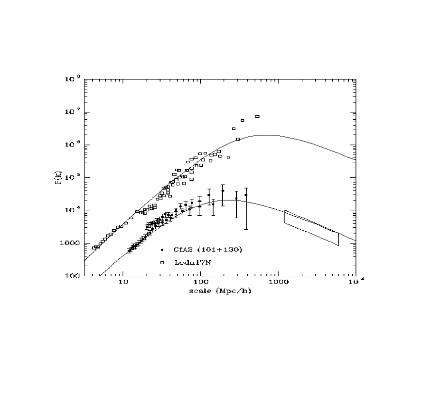
Figure 5: Power spectrum (PS) of several samples of LEDA together with the CfA2 power spectra (from [22] The amplitude of the PS depends on the sample depth, and it is larger in the case of LEDA, because in this case the effective depth is larger than the CfA2 one (see Table 1). The curved shape of the PS is also spurious that does not correspond to any intrinsic feature in the case of fractals, but it is only due to the finiteness of the sample volume [25]. We also plot a CDM-like fit both to the CFA2 data and the LEDA data. On the right, we plot the COBE data. No reasonable CDM curve can fit the data and COBE (from [25])

we report the power spectrum analysis (Fourier conjugate of $\xi(r)$) of some catalogues. Also in this case, as for $\xi(r)$, there is a specific dependence of the properties on the sample size, in full agreement with the direct correlation analysis of Fig.3. In particular, for a fractal structure, the amplitude of the power spectrum is a function of the sample size and the shape is characterized by a turnover: both these features, bending and scaling, are a manifestation of the finiteness of the survey volume, and cannot be interpreted as the convergence to homogeneity, nor to a power spectrum flattening. A detailed discussion of the power spectrum can be found in [27].

Essentially similar results have been obtained for the Abell and ACO cluster catalogues [1] [3] [2]. Also in these cases we observe a power law behaviour for the cluster correlations with $D\simeq 2$ and without any tendency towards homogenization up to $\sim 80h^{-1}Mpc$.

All these results imply that the previous ”correlation lengths” of $5h^{-1}Mpc$ and $25h^{-1}Mpc$, introduced for galaxies and clusters, are spurious and no real correlation length can be defined from the data. Therefore the much discussed mismatch between galaxy and cluster correlations, that is also at the basis of various theories for structure formation, does not actually exist. Cluster correlations correspond just to the continuation of galaxy correlations at larger scales. In the language of Statistical Physics, cluster catalogues are the coarse grained version of galaxy catalogues.

4 Statistical Validity of Catalogues

Often the concept of fair sample has been used to mean homogeneous sample. For this reason various samples are declared as not fair just because they are not homogeneous. We have seen instead that it was the method of analysis to be inappropriate while the samples are actually rather good in a statistical sense. This means that one can derive from them a statistically valid information about their correlation properties.

In relation to the statistical validity it is interesting to consider the IRAS catalogues because they seem to differ from all the other ones and to show some tendency towards homogenization at a relatively small scale Actually the point of apparent homogeneity is only present in some samples, it varies from sample to sample between $\sim 15\div 25h^{-1}Mpc$ and it is strongly dependent on the dilution of the sample. Considering that structures and voids are much larger than this scale and that the IRAS galaxies appear to be just where luminous galaxies are it is clear that this tendency appears suspicious. One of the characteristic of the IRAS catalogues with respect to all the other ones is an extreme degree of dilution: this catalogue contains only a very small fraction of all the galaxies. It is important therefore to study what happens to the properties of a given sample if one dilutes randomly the galaxy distribution up to the IRAS limits. A good test can be done by considering the Perseus Pisces catalogue and eliminating galaxies from it. The original distribution shows a well defined fractal behavior. By diluting it to the level of IRAS one observes an artificial flattening of the correlations [28] (see Fig.6).

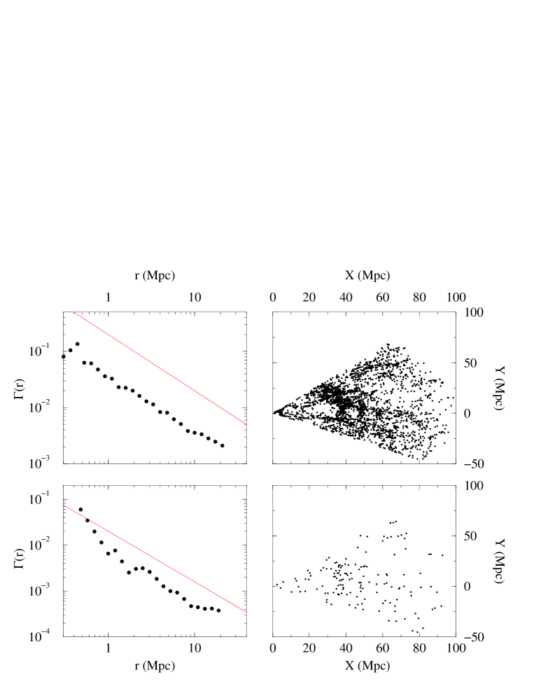
Figure 6: Top panels: The conditional density (left) for a volume limited sample of the full Perseus-Pisces redshift survey (right). The percentage of galaxies present in the sample is $\sim 6\%$. The slope is $-\gamma=-1$. Bottom panels: In this case the percentage of galaxies is $\sim 1\%$, and the number of galaxies is the same of the IRAS $1.2Jy$ sample in the same region of the sky. We can see that at small scale we have a $1/r^{3}$ decay just due to the sparseness of the sample, while at large scale the shot noise of the sparse sampling overcomes the real correlations and produces an apparent trend to homogenization [27]. In our opinion, this effect, due to sparsness of this sample, is the origin of the apparent trend towards homogeneization observed in some of the IRAS samples.

This effect does not correspond to a real homogenization but it is due to the of dilution. In fact it can be shown that when the dilution is such that the average distance between galaxies becomes comparable with the largest voids (lacunarity) of the original structure there is a loss of correlation and the shot noise of the sparse sampling overcomes the real correlations and produces an apparent trend to homogenization [27]. This allows us to reconcile this peculiarity of the IRAS data with the properties of all the other catalogues. Analogous considerations for other sparse samples like QDOT and the Stromlo-APM samples [2].

The correlations discussed up to now are well defined statistically but limited to the radius of the largest sphere that can be contained in the sample $R_{s}$. For example for Las Campanas the depth is very large $R_{d}\sim 500h^{-1}Mpc$ but $R_{s}$ is only $20h^{-1}Mpc$ because the sample is very thin. So, it is not surprising that the value of $r_{0}$ is also small ($6\div 7h^{-1}Mpc$). Given this situation it would be very interesting to find some method that is limited by $R_{d}$ instead of $R_{s}$.

Galaxy samples have typically a conic shape and, in this respect, they are three dimensional objects. Considering a volume limited sample, if one simply counts the number of galaxies within a distance $r$ from the vertex this number should go like $r^{3}$ for a homogeneous distribution and like $r^{D}$ for a fractal one. In order to compare with the previous correlation analysis it is actually convenient to consider the density instead of the total number. The problem with such an analysis is that one cannot average from different observational points but the count is from a single point, the vertex. This situation corresponds to a reduced statistical quality that should be carefully analyzed.

At very small distances we are not going to find any point. When a distance of the order of the minimal one between galaxies is reached, we begin to have a signal but this is strongly affected by finite size effects as shown schematically in the insert of Fig.3. Eventually at some distance $\lambda$, the number of points becomes large enough that one reaches the correct scaling behavior. It can be shown that this characteristic length for the statistical significance of this method is about ten times the minimal distance between galaxies. For various catalogues the value of $\lambda$ is appreciably smaller that $R_{d}$ and, in these cases, a useful information can be obtained for the length scales between $\lambda$ and $R_{d}$. A detailed discussion of this method can be found in [28]. This approach is quite useful because it allows us to use the thin deep catalogues up to their total depth $R_{d}$. Particularly interesting in this respect is the ESP catalogue whose depth extends up to $900h^{-1}Mpc$. Also for the Las Campanas sample it is possible to obtain some information despite the peculiar and unfortunate luminosity selections of this catalogue. The results of these deep catalogue are reported in Fig.3 together with those of the other catalogues discussed before. The amplitude of the density computed from the vertex for all the catalogues is systematically shifted by about a factor of 3 (that has been rescaled in Fig.3) with respect to the full correlation analysis. This shift is due to the fact that usually, observations point towards zones that are rich of galaxies. A detailed discussion of this effect is reported in [2].

The behaviour of the density decay from the vertex shows the same power law behavior of the full correlation analysis of Fig.3 (left part) but this property is now shown to extend up to $900h^{-1}Mpc$. The agreement between different catalogues and different methods of analysis is remarkable and it shows a well defined fractal behavior for the galaxy correlations extending from $1$ to about $1000h^{-1}Mpc$ (Fig.3). This analysis refutes therefore the early comments about a possible homogenization in Las Campanas, based on the visual impression of the data.

In relation to the lecture by Prof. Davis, it should be noted that the function $n(z)$ (redshift counts in a magnitude limited sample) it can be shown [2] that the behaviour of such a quantity is mostly related to the luminosity selection function of the survey rather than to the behaviour of the space density. In particular, such a quantity cannot be used to distinguish between fractal or homogeneous properties of the galaxy distribution.

5 Number Counts and Angular Correlations

The above discussion of the density decay from the vertex brings us naturally to the problem of the galaxy number counts that is also performed in this way, namely by counting from the origin. There are however some relevant differences because all the properties discussed up to here refer to volume limited samples while the galaxy counts are defined by their apparent magnitude. The behaviour of the number versus magnitude relation ($N(<m)$) is reported in Fig.7.

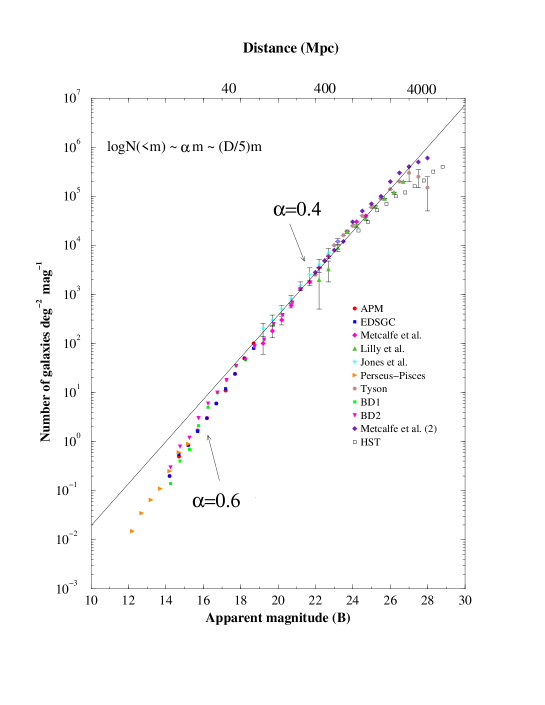
Figure 7: The galaxy number counts in the $B$-band, from several surveys. In the range $12\mathrel{\hbox to0.0pt{\lower 3.0pt\hbox{$\mathchar 536\relax$}\hss}\raise 2.0pt\hbox{$\mathchar 316\relax$}}m\mathrel{\hbox to0.0pt{\lower 3.0pt\hbox{$\mathchar 536\relax$}\hss}\raise 2.0pt\hbox{$\mathchar 316\relax$}}19$ the counts show an exponent $\alpha\simeq 0.6\pm 0.1$, while in the range $19\mathrel{\hbox to0.0pt{\lower 3.0pt\hbox{$\mathchar 536\relax$}\hss}\raise 2.0pt\hbox{$\mathchar 316\relax$}}m\mathrel{\hbox to0.0pt{\lower 3.0pt\hbox{$\mathchar 536\relax$}\hss}\raise 2.0pt\hbox{$\mathchar 316\relax$}}28$ the exponent is $\alpha\simeq 0.4$. The amplitude of the galaxy number counts for $m\mathrel{\hbox to0.0pt{\lower 3.0pt\hbox{$\mathchar 536\relax$}\hss}\raise 2.0pt\hbox{$\mathchar 318\relax$}}19$ (solid line) is computed from the determination of the prefactor $B$ of the density $n(r)=Br^{D-3}$ (with $D=2$ - see text) at small scale and from the knowledge of the galaxy luminosity function. The distance is computed for a galaxy with $M=-16$ and we have used $H_{o}=75kmsec^{-1}Mpc^{-1}$ [27] [2].

The exponent $\alpha$ defined by this relation can be related to the dimension $D$ of the galaxy distribution ($\alpha=D/5$). For small magnitudes (small scales), one observes $\alpha\simeq 0.6\pm 0.1$ that is usually interpreted as evidence of homogeneity ($D\approx 2$). At larger scales the value of $\alpha$ decreases to about $0.4$ (corresponding to $D\simeq 2$) and this deviation is considered as due to galaxy evolution and solid angle effects due to the expansion. However, from the direct correlation analysis in 3-d space, we know that up to some rather large scale the galaxy distribution is certainly fractal. Therefore the usual interpretation of $\alpha\simeq 0.6\pm 0.1$ at small scales in terms of a homogeneous distribution cannot be correct. In this respect the insert of Fig.3 allows us to clarify the situation. In fact, at relatively small scales, the density first raises and then falls when it reaches the correct scaling regime. This behaviour can roughly resemble a constant density, especially for an integrated quantity. A variety of tests for various catalogues with fractal correlations in 3-d, like the Perseus Pisces survey and others, show that the number counts give indeed an exponent $\alpha\simeq 0.6\pm 0.1$ if the sample is dominated by small scales finite size fluctuations. On the other hand, if one computes the number counts by performing an average over all the different observers in a redshift sample, the value $\alpha\approx 0.4$ is readily found, in agreement with the space correlation analysis. In the deep surveys ($m\mathrel{\hbox to0.0pt{\lower 3.0pt\hbox{$\mathchar 536\relax$}\hss}\raise 2.0pt\hbox{$\mathchar 318\relax$}}19$) the small scale fluctuations are self-averaging so that one can recover the correct properties (i.e. $\alpha\approx 0.4$) without performing any average.

This implies a completely different interpretation of the number counts. At small scales the value $\alpha\approx 0.6$ is due to finite size effects and not to a real homogeneity, while at larger scales the value 0.4 corresponds to the correct correlation properties of the sample. This implies that galaxy evolution, modification of the Euclidean geometry and the K-corrections are not very relevant in the range of the present data. In addition the fact that the exponent 0.4 holds up to magnitudes $27\div 28$ seems to indicate that the fractal properties may extend up to $2\div 3000h^{-1}Mpc$. The amplitude of the galaxy number counts for $m\mathrel{\hbox to0.0pt{\lower 3.0pt\hbox{$\mathchar 536\relax$}\hss}\raise 2.0pt\hbox{$\mathchar 318\relax$}}19$ (see the solid line Fig.7) is computed from the determination of the prefactor $B$ of the density $n(r)=Br^{D-3}$ at small scale and from the knowledge of the galaxy luminosity function [28]. Quite a remarkable fact if one considers that the Hubble radius of the universe is supposed to be $4000h^{-1}Mpc$. Such a behaviour ($\alpha\sim 0.4$, i.e. $D\sim 2$) can be found for galaxies in the different Photometric bands, as well as for other astrophysical objects [28].

We have now all the elements to reinterpret also the angular catalogues. These catalogues are qualitatively inferior to the 3-d ones because they only correspond to the angular projection and do not contain the third coordinate. However the fact that they contain more points with respect to the 3-d catalogues has led some authors to assign an excessive importance to these catalogues (once we have the 3-d ones). In fact, even for a very large number of points ($N\rightarrow\infty$) the angular distribution is intrinsically degenerate, in the sense that it can originate from different 3-d distributions. Actually the interpretation of the angular catalogues is quite delicate and ambiguous for a variety of reasons:

- Unlike orthogonal projections, angular projections mix different length scales and this gives an artificial randomization of the points. This can be illustrated as follows: consider a small solid angle $d\Omega$ of an angular catalog. This will contain the projection of all the points in the corresponding cone of depth $R_{d}$. This cone is a three dimensional object, so the intersection with a fractal of dimension $D$ will also be a set of dimension $D$. Therefore the number of points that project in $d\Omega$ is $N(d\Omega,R_{d})\sim d\Omega R_{d}^{D}$. This implies that for a large enough value of $R_{d}$ any small solid angle $d\Omega$ will contain some points. This is why structures and voids are smeared by the angular projection. This implies that the angular projection of a fractal structure can be really homogeneous at relatively large angles [1] [29] [2]. Clearly this is an artificial effect and from a smooth angular projection one cannot deduce whether the real distribution is also smooth. An example of this effect is given by Fig.2 in which the angular projection appears relatively smooth, while the real distribution is much more irregular. In fact the large structures and large voids have been identified with the redshift catalogues and could not be predicted from the angular data alone.

- An additional effect is the one due to the finite size effects discussed before in case of a single observational point that gives an additional artificial effect of homogenization. The so called rescaling of the angular correlations can be understood in detail by these effects and it can be shown that the same properties can be observed in a fractal distribution [28].

Concerning the debate with M. Davis and the subsequent discussion with J. Peebles it should be noted that the angular projections correspond to a complex convolution with the magnitude limit and dilution effects in the case of IRAS. Contrary to the claim of M. Davis we have already analyzed the propreties of angular projections [29] [1] [2] and identified a number of problems, like those mentioned here, that were not known before and that make these catalogues intrinsically unambiguous. For these reasons we decided to focus on 3-d distributions that lead to the consistent and ambiguous results shown in Fig.3. Concerning the proposal of Davis and Peebles to generate a fractal distribution in 3-d that corresponds to the observed angular projections, this requires the tuning of various other properties in addition to the fractal dimension. In particular lacunarity, morphology, magnitude limits and dilution effects all play a crucial role in the projection and should be tuned to those of real galaxies. In any case 3-d galaxy distributions are fractals and their properties do not depend on our ability to make this exercise.

6 Luminosity and Space Distribution

Up to now we have discussed galaxy correlations only in terms of the set of points corresponding to their position in space. Galaxies can be also characterized by their luminosity (related to their mass) and the full luminosity distribution is then a full distribution and not a simple set. It is natural then to consider the possible scale invariant properties of this distribution. This requires a generalization of the fractal dimension and the use of the concept of multifractality [4]. In this language the fractal set discussed until now represents the support of the full luminosity distribution.

A multifractal analysis shows that also the full distribution is scale invariant [1] [22] and this leads to a new and important relation between the Schechter luminosity distribution and the space correlation properties. This allows us to understand various morphological features (like the fact that large elliptic galaxies are typically located in large clusters) in terms of multifractal exponents. This leads also to a new interpretation of what has been called the luminosity segregation effect [30].

The observation that the most luminous elliptical galaxies lie in the core of rich galaxy clusters is, in our analysis, a manifestation of the multifractal properties, i.e. the self-similar distribution of matter including galaxy masses (luminosities). However this observation together with the shift of $r_{0}$ with sample depth (interpreted as luminosity limit) has lead various authors [31] [23] [32] to formulate the qualitative hypothesis that the homogenization crossover (related to $r_{0}$) should be different for galaxies of different luminosity. The fact that large voids ($\mathrel{\hbox to0.0pt{\lower 3.0pt\hbox{$\mathchar 536\relax$}\hss}\raise 2.0pt\hbox{$\mathchar 318\relax$}}50h^{-1}Mpc$) are empty of galaxies of any type is already a disproof of this hypothesis. In addition we have shown that the appropriate correlation analysis shows a power law behaviour at any observable scale. This implies unavoidably that $r_{0}$ must scale with the sample size because the system is self-similar. Most of the analysis of the luminosity segregation effects usually do not address the fundamental question whether $r_{0}$ is a physical meaningful quantity, that should be addressed with the conditional density. Only once a crossover towards homogeneity would be observed in the conditional density then ”luminosity segregation” questions could eventually be posed in the usual terms.

7 Conclusions and Theoretical Implications

In summary our main points are:

• The highly irregular galaxy distributions with large structures and voids strongly point to a new statistical approach in which the existence of a well defined average density is not assumed a priori and the possibility of non analytical properties should be addressed specifically.

• The new approach for the study of galaxy correlations in all the available catalogues shows that their properties are actually compatible with each other and they are statistically valid samples. The severe discrepancies between different catalogues that have led various authors to consider these catalogues as not fair, were due to the inappropriate methods of analysis.

• The correct two point correlation analysis shows well defined fractal correlations up to the present observational limits, from 1 to $1000h^{-1}Mpc$ with fractal dimension $D\simeq 2$. Of course the statistical quality and solidity of the results is stronger up to $100\div 200h^{-1}Mpc$ and weaker for larger scales due to the limited data. It is remarkable, however, that at these larger scales one observes exactly the continuation of the correlation properties of the small and intermediate scales.

• These new methods have been extended also to the analysis of the number counts and the angular catalogues which are shown to be fully compatible with the direct space correlation analysis. The new analysis of the number counts suggests that fractal correlations may extend also to scales larger that $1000h^{-1}Mpc.$

• The inclusion of the galaxy luminosity (mass) leads to a distribution which is shown to have well defined multifractal properties. This leads to a new, important relation between the luminosity function and that galaxy correlations in space.

• New perspective on old arguments. On the light of these results we can now take a standard reference volume in the field (i.e. Peebles 1993 [5]) and consider the usual arguments invoked for homogeneity from a new point of view. These arguments are: (a) number counts: we have seen in Sec.5 that the small scale exponent of number counts is certainly not related to homogeneity but to small scale fluctuations. The real exponent of the number counts is instead the lower one (i.e. $\alpha\approx 0.4$) that indeed corresponds to the three dimensional (i.e fractal with $D\simeq 2$) correlation properties. (b) $\delta N/N$ is small for various observations. This point is exactly the same as the fact $r_{0}$ is a spurious length. In the absence of a reference average one cannot talk about ”large” or ”small” amplitude of fluctuations. In addition, for any distribution, even a fractal one $\delta N/N$ is always small for sizes comparable to the total sample because the average is computed from the sample itself. (c) Angular correlations. We have seen in Sec.5 that angular correlations are ambiguous in two respects: first the angular projection of a fractal is really uniform at large angles due to projection effects, second the angular data are strongly affected by the finite size fluctuations that provide an additional artificial homogenization, as in the case of the number counts. The inclusion of these effects reconciles quite naturally the angular catalogs with the fractal properties in the three dimensional ones. (d) X-ray background. The argument that $\delta N/N$ becomes very small for the X-ray background combines the two problems discusses before: angular projections and reference average. This angular uniformity is analogues, for example, to the Lick angular sample, and certainly is not a proof of real homogeneity.

  Finally one should note that all these arguments are indirect and always require an interpretation based on some assumptions. The most direct evidence for the properties of galaxy distribution arises from the correct correlation analysis of the 3-d volume limited samples that has been the central point of our work.

Theoretical Implications

From the theoretical point of view the fact that we have a situation characterized by self-similar structures implies that we should not use concept like $\xi(r)$, $r_{0}$, $\delta N/N$ and certain properties of the power spectrum, because they are not suitable to represent the real properties of the observed structures. In this respect also the N-body simulations should be considered from a new perspective. One cannot talk about ”small” or ”large” amplitudes for a self-similar structure because of the lack of a reference value like the average density. The Physics should shift from ”amplitudes” towards ”exponent” and the methods of modern statistical Physics should be adopted. This requires the development of constructive interactions between two fields.

Possible Crossover. We cannot exclude of course, that visible matter may really become homogenous at some large scale not yet observed. Even if this would happen the best way to identify the eventual crossover is by using the methods we have described and not the usual ones. From a theoretical point of view the range of fractal fluctuations, extending at least over three decades ($1\div 1000h^{-1}Mpc$), should anyhow be addressed with the new theoretical concepts. Then one should study the (eventual) crossover to homogeneity as an additional problem. For the moment, however, no tendency to such a crossover is detectable from the experimental data and it may be reasonable to consider also more radical theoretical frameworks in which homogenization may simply not exist at any scale, at least for luminous matter.

Dark Matter. All our discussion refers to luminous matter. It would be nice if the new picture for the visible universe could reduce, to some extent, the importance of Dark matter in the theoretical framework. At the moment however this is not clear. We have two possible situations: (i) if Dark matter is essentially associated to luminous matter, then the use of FRW metric is not justified anymore. This does not necessarily imply that there is no expansion or no Big Bang. It implies, however, that these phenomena should be described by more complex models. (ii) If Dark matter is homogenous and luminous matter is fractal then, at large scale, Dark matter will dominate the gravity field and the FRW metric is again valid. The visible matter however remains self-similar and non analytical and it still requires the new theoretical methods mentioned before. However, this perspective seems to be in contrast with the usual role of Dark Matter, that is to generate large potential wells for the initially smoother baryonic matter.

Predictions and Bets

After the debate with Prof. M. Davis, we tried to assess the predictions of the two points of view and we also agreed to make a bet. According to the arguments of Prof. M. Davis, the length $r_{0}\simeq 5h^{-1}Mpc$ characterizes the physical properties of galaxy distributions. Therefore deeper samples like CfA2 and SLOAN should simply reduce the error bar, which is now about considered to be $10\%$. A possible variation of $r_{0}$ with absolute magnitude, due to a luminosity bias (see Sec.6), is considered plausible but it has never been quantified. This should be checked by varying independently absolute magnitude and depth of the volume limited samples. However, from this interpretation, the value of $r_{0}=5h^{-1}Mpc$, corresponding to a volume limited of CfA1 with $M=-19.5$, should not change when considering in CfA2 and SLOAN volume limited samples with the same solid angle $\Omega$ and the same absolute magnitude limit ($M=-19.5$).

In our interpretation, instead, $r_{0}$ is spurious, and it scales linearly with the radius $R_{s}$ of the largest sphere fully contained in the volume limited samples. Therefore we predict for the volume limited sample of CfA2 with $M=-19.5$ (with a solid angle of $\Omega=1.1\;sr$ [23]) $r_{0}\approx 7h^{-1}Mpc$ (if, in the final version of the survey the solid angle will be $\Omega=1.8$, the value of $R_{s}$ will increase accordingly, and the value of $r_{0}$ will shift up to $\sim 9h^{-1}Mpc$). Note however that for the deepest volume limited CfA2 sample ($M\mathrel{\hbox to0.0pt{\lower 3.0pt\hbox{$\mathchar 536\relax$}\hss}\raise 2.0pt\hbox{$\mathchar 316\relax$}}-20$) we predict instead $r_{0}\approx 15\div 20h^{-1}Mpc$. For the volume limited sample of the full SLOAN with $M=-19.5$ ($\Omega=\pi$), our prediction is that $r_{0}\approx 65h^{-1}Mpc$. It is clear that however, the first SLOAN slice will give smaller values because the solid angle will be small.

About the respective predictions for the full SLOAN ($\Omega=\pi\;sr$) one of us (L.P.) made a bet with Prof. M. Davis [33] (of a case of Italian or Californian wine). The predictions are $r_{0}\simeq 5h^{-1}Mpc$ (Davis) and $r_{0}\mathrel{\hbox to0.0pt{\lower 3.0pt\hbox{$\mathchar 536\relax$}\hss}\raise 2.0pt\hbox{$\mathchar 318\relax$}}50h^{-1}Mpc$ (for the volume limited samples with $M<-19.5$), so the threshold for the bet was set (by the referee N. Turok) to be the geometric average between the values: $r_{0}=15h^{-1}Mpc$.

References

- [1] Coleman, P.H. and Pietronero, L.,1992 Phys.Rep. 231,311
- [2] Sylos Labini, F., Montuori, M.and Pietronero,L. 1996, preprint
- [3] Montuori, M., Sylos Labini, F. and Amici, A. 1996, preprint
- [4] Pietronero L., Physica A, 144, 257
- [5] Peebles, P.E.J., 1980 ”The Large Scale Structure of The Universe” (Princeton Univ.Press.); Peebles, P.E.J. 1993 ”Principles of physical Cosmology” (Princeton Univ.Press.)
- [6] Weinberg, S. E. 1972 ”Gravitation and Cosmology” Wiley, New York.
- [7] Wilson K.G., 1974 Phys. Rep. 12, 75
- [8] Amit D., 1978 ”Field theory, the Renormalization Group and Critical Phenomena (Mc Graw-Hill, New York)
- [9] Mandelbrot B., 1982 The Fractal Geometry of Nature, Freeman, New York
- [10] Erzan A, Pietronero L., Vespignani A. Rev. Mod. Phys. 1995, 67, 554
- [11] Sylos Labini, F., 1994, Ap.J., 433, 464
- [12] De Lapparent, V., Geller, M. J., Huchra, J. P. (1988) Ap.J. 332, 44
- [13] Davis, M., Peebles, P. J. E. 1983 Ap.J., 267,465
- [14] Huchra, J., Davis, M., Latham, D., Tonry, J. 1983 Ap.J.S, 52, 89.
- [15] Coleman, P.H. Pietronero, L.,& Sanders,R.H.,1988, A&A, 245,1
- [16] Bahcall N. A. & Soneira R. M., 1983, ApJ, 270, 20
- [17] Baryshev, Y., Sylos Labini, F., Montuori, M., Pietronero, L. Vistas in Astron. 1994, 38, 419
- [18] Strauss M.A., et al., 1992 Ap.J.S 83, 29; Fisher K. et al.1995 Ap.J. Suppl. 100, 69
- [19] Fisher K., et al 1994 MNRAS 266, 507
- [20] Da Costa L.N., et al.1991, ApJ. Suppl.,91, 935
- [21] Loveday J., 1996 MNRAS, 278, 1025
- [22] Sylos Labini, F., Montuori, M., Pietronero,L. 1996, Physica A, 230, 368; Di Nella H., Montuori M., Paturel G., Pietronero L., and Sylos Labini F., Astron.Astrophys.Lett. 1996, 308, L33
- [23] Park, C., Vogeley, M.S., Geller, M., Huchra, J. 1994 Ap.J., 431, 569;
- [24] Haynes, M., Giovanelli, R., 1988 Large-scale motion in the Universe, ed. Rubin, V.C., Coyne, G., Princeton University Press, Princeton; Paturel, G., Bottinelli, L., Gouguenheim, L., Fouque, P. 1988 A&A, 189, 1; Vettolani, G., et al. (1994) Proc. of Scloss Rindberg workshop Studying the Universe with Clusters of Galaxies; Schectman et al., 1996 Ap.J. 470, 172
- [25] Baryshev, Y., Pietronero, L, Sylos Labini, F. & Teerikorpi P., 1996 preprint
- [26] Amendola L, Di Nella H., Montuori M., and Sylos Labini F., 1996 preprint
- [27] Sylos Labini, F. Amendola, L. 1996, Ap.J. Lett, 468, L1
- [28] Sylos Labini, F., Gabrielli, A., Montuori, M., Pietronero,L. 1996, Physica A, 266, 149
- [29] Dogterom M. and Pietronero L., 1991 Physica A, 171, 239
- [30] Sylos Labini, F., Pietronero,L. 1996. Ap.J. 469, 28
- [31] Davis M. et al., 1988 ApJ Lett 333, L9
- [32] Benoist C. et al.1996 ApJ in print
- [33] Davis M., in these Proceedings (astro-ph/9610149)