The Physics of Type Ia Supernova Lightcurves:
I. Opacity and Diffusion

Abstract

We examine the basic physics of type Ia supernova (SNe Ia) light curves with a view toward interpreting the relations between peak luminosity, peak width, and late-time slope in terms of the properties of the underlying explosion models. We develop an analytic solution of the radiation transport problem in the dynamic diffusion regime and show that it reproduces bolometric light curves produced by more detailed calculations under the assumption of a constant extinction coefficient. This model is used to derive the thermal conditions in the interior of SNe Ia, to address the issue of time dependence in the modeling of SNe Ia light curves and spectra and to show that these are intrinsically time-dependent phenomena. The analytic model is then used to study the sensitivity of light curves to various properties of supernova explosions. We show that the dominant opacity arises from line transitions and discuss the nature of line opacities in expanding media and the appropriateness of various mean opacities used in light curve calculations.

1 Introduction

The bolometric light curve is the simplest and most direct manifestation of type Ia supernovæ (hereinafter SNe Ia). For many years it had been assumed that all Type Ia supernovæ (hereinafter SNe Ia) were identical explosions, with identical light curve shapes and peak luminosities (c.f. WoosleyW86). While evidence for this uniformity in the data was never terribly convincing, the use of SNe Ia as the primary “standard candles” for cosmological distance measurement provided a powerful incentive for assuming this homogeneity. This in turn lead naturally to a search for an explosion model which might produce identical displays from the diversity of progenitors supplied by stellar evolution.

It became clear from the light curve’s rapid evolution that a relatively low mass object was involved, one with a short radiative diffusion time Arnett (1982). The result of this search is what one might call the present “standard model”, the thermonuclear incineration of a carbon-oxygen white dwarf at the Chandrasekhar mass (see WoosleyW86, Arnett96 for details of this search and a review of various models). The Chandrasekhar mass provides a point of convergent evolution for various progenitor systems, offering a natural explanation of the assumed uniformity of display. The high densities attained at the centers of these objects provides as well a mechanism (as ill-defined as it may be at present) for their ignition.

With the coming of age of various supernova searches, (Hamuyetal93, Pollas94, EvansVM89, BarbonBCPT93) there has recently been an explosion in the availability of high-quality data. It is now generally recognized that SNe Ia exhibit a variety of light curve shapes, peak luminosities, and maximum-light spectra. Perhaps most significant has been the discovery of various regularities in the light curve data, the most famous of which we will call the “Phillips Relation” (hereinafter PR) Phillips (1993); the brightest supernovæ have the broadest light curve peaks. There is also significant evidence (VaccaL96a) that the decline at late times is more gradual in the brighter supernovæ.

This additional information provides new clues to the nature of these explosions. We develop here, from first principles, a theoretical framework for examining the formation of SNa Ia light curves and extracting underlying properties of the explosions. While there have been a number of studies of the light curve problem in SNe Ia (HoflichKW95 and references therein, WeaverAW80), none has included a detailed examination of the physics of the opacity or radiation transport in these explosions.

We divide the present investigations into four parts. In the first we derive an analytic solution for the co-moving frame transfer equation in homologous expansion. We use this solution to examine the relative importance of various terms in the equations and the suitability of various approximations which have appeared in the literature. The analytic solution also provides an important check on the accuracy of our subsequent numerical solutions.

In the second part we examine the nature of the opacity. SNe Ia differ significantly from other astrophysical objects in their composition; they are entirely constituted of heavy elements. This allows a number of interesting effects, present at a low level in all objects, to take on a dominant role. We find that the extreme complexity of the atomic physics allows for a transport of energy downward in frequency which has a profound effect upon the radiative diffusion time. This transport also allows for a process, akin to thermalization but not mediated by collisions, which can lead to a spectrum which appears thermal but which need have little to do with the gas temperature anywhere in the object.

In the third part we present several light curves calculated by solving the time-dependent, multi-frequency transport equations. We use these detailed solutions to examine the behavior of the mean opacity, and find that the most natural a priori choice, the Rosseland mean, significantly underestimates the true flux mean by up to a factor of five. The flux mean appears to be, at least in LTE, remarkably constant both in time and in radius.

Finally, we exploit the constancy of the flux mean to examine the effect of varying the bulk parameters of the explosion on the shape of the light curve. For present purposes, SNe Ia can be characterized by specifying density and composition as a function of ejecta velocity. We will ignore, at least to begin with, how this structure was brought about. We will also ignore any departures from spherical symmetry—as will be seen, the problem is vexing enough in one spatial dimension. We note however that Wang et al. 1996 found no evidence for polarization in their study of three SNe Ia, nor has there been any other evidence from optical polarimetry for gross asphericity in SNe Ia explosions.

The post-explosion dynamics, which determine the density and velocity structure, are quite simple. As in all strong point explosions, the expansion becomes homologous after a time which is short compared with the bolometric rise-time, with a velocity gradient everywhere equal to the reciprocal of the elapsed time. The density structure is quite smooth, with a density profile not very different from $\rho\propto\exp(-4v/v_{0})$ (with $v_{0}$ some typical velocity $\propto(E/M)^{1/2}$). There is usually a small amount of high-velocity material at the surface in which the density drops more rapidly; as this material is largely transparent long before the supernova is observed we may ignore this detail. To a surprising degree, all explosion models to date have this relatively simple structure. Thus, the dynamics can be specified by the explosion energy and the mass of the ejecta (in most models the progenitor is completely disrupted).

The other defining attributes of the explosion are in the composition of the ejecta. Since it is radioactive nickel which leads to any optical display at all, the amount of ⁵⁶Ni and the depth to which it is buried in the ejecta will obviously affect the light curve. The composition also affects the opacity, obviously a determining parameter in a problem concerning the escape of radiation.

We will thus define a supernova by its total mass, explosion energy, ⁵⁶Ni mass and opacity, possibly allowing for variations in the spatial distribution of the latter two (we will find that this is relatively unimportant). With a simple means of producing a light curve from these four parameters, one may turn the problem around and use the light curve model to extract values for these parameters from observations of SNe Ia.

We find that, with the exception of the total mass, variations in any of these basic parameters lead to a behavior of the light curve which is in the opposite sense of the PR. Varying the total mass, however, can lead to a sequence of light curves in which the PR behavior is reproduced. This is by no means a proof that the full richness of SN Ia light curve behavior cannot be obtained from Chandrasekhar mass explosions. It does however suggest that the total mass of the explosion may be a natural and simple explanation for observations.

This is the first paper of a series. The next paper Pinto & Eastman (1996) explores the lightcurve behavior of simple models for SNe Ia. Subsequent papers will systematically explore the light curve and spectrum properties of specific models for Type Ia supernovae.

2 A Schematic Type Ia Supernova

In this section we develop a simple analytic model for the thermal evolution and light curve of a SN Ia. This will prove useful for estimating physical conditions in the ejecta at various times after explosion, and for illustrating the effect which changes in opacity, mass, energy deposition, and explosion energy have on the bolometric light curve.

The ejecta of SNe Ia form an opaque, expanding sphere into which energy is deposited by radioactive decay at an exponentially-declining rate. Because the sphere is initially so opaque, this energy is converted into kinetic energy of expansion on a hydrodynamic timescale. At the earliest stages the ejecta is so optically thick that the time it takes radiation to diffuse out is much longer than the elapsed time. The luminosity is therefore initially quite small. As time passes, the ejecta become more dilute and the diffusion time drops below the (ever-increasing) elapsed time. Since the rate of energy input declines exponentially with time, there is a peak in the light curve as soon as the injected energy has an appreciable chance to escape conversion to kinetic energy—when the diffusion time becomes comparable to the elapsed time. While the fraction of deposited energy which escapes conversion will continue to increase, this is more than offset by the decreasing energy deposition rate.

Shortly after this peak, there will be a considerable amount of radiation still trapped and diffusing outward. Since the energy deposition rate is so rapidly declining, the luminosity will, for a time, exceed the rate of deposition until the supernova empties itself of this excess stored energy. Finally, as the rate of energy deposition, now from cobalt decay, declines more slowly and the diffusion time becomes small, the luminosity becomes equal to the instantaneous deposition rate. There are thus two milestones in the light curve. The first occurs near peak when the luminosity first rises above the rate of energy deposition. The second occurs when the excess, stored energy is exhausted and the luminosity falls to equal the instantaneous deposition. The elapsed time and the rate of deposition are easily determined. The first is obvious and the second comes from the decay of ⁵⁶Ni to ⁵⁶Fe and the transport of $\gamma$-rays – fairly simple physics. Determining the diffusion time is a far more complex matter, and most of the difficulty in producing synthetic light curves and spectra arises from correctly characterizing the transport and escape of thermalized radiation.

Arnett showed in two elegant papers (Arnett80; Arnett82) that the ideas expressed above could be demonstrated by a simple analytic model which accounts for the deposition and escape of radiation from the expanding ejecta. This model predicted a bolometric light curve which was generically in good agreement with observed Sn Ia behavior. Starting from the thermodynamics of the trapped radiation, he showed that the luminosity at peak was equal to the instantaneous energy deposition rate under the assumption of constant opacity, and thus the first milestone occurs near peak bolometric luminosity. A number of assumptions were made which, for a first attempt, were quite reasonable, but which rendered suspect the precise predictions for any particular model explosion. These included a constant density structure, a constant opacity in both space and time, and the requirement that the radial distribution of the energy deposition was identical to that of the thermal energy. Thus, while he could vary the expansion velocity and the total mass, the effects of varying the structure of the ejecta and of a realistic energy deposition profile were beyond examination. In mathematical terms, Arnett’s solution was an eigenfunction expansion from which only the fundamental mode is retained. We shall have more to say on this later.

We take a no-frills approach similar to Arnett’s 1982, while relaxing some of his more limiting assumptions so as to be able to address additional questions such as how the density structure and distribution of radioactive isotopes are manifested in the bolometric light curve.

We start by writing down the first two frequency-integrated moments of the time dependent, co-moving frame radiative transport equation in spherical geometry. The first moment equation, for the radiation energy density, can be written, correct to all terms O(v/c), as (cf. MihalasM84)

$${{DE}\over{Dt}}+{1\over{r^{2}}}{{\partial}\over{\partial r}}\left(r^{2}F\right)+{v\over r}\left(3E-P\right)+{{\partial v}\over{\partial r}}\left(E+P\right)=\int_{0}^{\infty}\left[4\pi\eta_{\nu}-c\chi_{\nu}E_{\nu}\right]d\nu.$$ (1)

The second frequency-integrated moment, for the radiation momentum, is

$${1\over{c^{2}}}{{DF}\over{Dt}}+{{\partial P}\over{\partial r}}+{{3P-E}\over r}+{2\over{c^{2}}}\left({{\partial v}\over{\partial r}}+{v\over r}\right)F=-{1\over c}\int_{0}^{\infty}\chi_{\nu}F_{\nu}d\nu.$$ (2)

Here $E$, $F$, and $P$ are the zero, first, and second frequency-integrated moments of the radiation field: the energy density, the flux, and the (isotropic) radiation pressure. $\chi_{\nu}$ is the extinction coefficient, and $\eta_{\nu}$ is the volume emissivity. These are formidable equations to solve directly (cf. EastmanP93 among others) and our goal here is to obtain a simple and approximate solution.

The first and most important approximation we will employ is that the expansion is homologous. As already described, SNe Ia are strong point explosions; homologous expansion will be an excellent approximation if the energy released by ⁵⁶Ni decay does not strongly affect the dynamics of the expansion. The energy available from ⁵⁶Ni decay is $3\times 10^{16}$erg g^-1. This corresponds to the kinetic energy of a gram of material traveling at nearly 2500 km s^-1, or, equivalently, a velocity increment of the same magnitude over the velocity initially imparted by the explosion. The significantly greater decay energy available from decay all the way to ⁵⁶Fe is less relevant as most of the ⁵⁶Co decay energy is emitted at times when the supernova is becoming optically thin. Since the observed expansion velocity of SNe Ia is in excess of $10^{4}$ km s^-1, we expect that this additional source of energy will have a modest, but perhaps not completely negligible, effect upon the velocity structure. Furthermore, as the time to maximum light, $t_{max}$, is observed to be at least twice as large the ⁵⁶Ni decay time, most of the hydrodynamic effect of ⁵⁶Ni  decay will have occured prior to a supernova’s discovery. If we take the ejecta’s density structure from an explosion calculation which has allowed this additional energy to accelerate the ejecta for the first few days we will have taken this effect sufficiently into account. We will therefore take the outer edge of the supernova, or at least of a fiducial mass shell which contains virtually all of the mass, to be at a velocity $v_{max}$ and a radius

$$R(t)=R_{0}+v_{max}t$$ (3)

where $R_{0}$ is the initial radius of the progenitor. For this type of expansion law there is an associated time scale

$$t_{sc}=R_{0}/v_{max}.$$ (4)

which will be one of the parameters of the solution.

A major simplification is the so-called Eddington Approximation, wherein the radiation field is everywhere isotropic: $E=3P$. This is certainly valid during the early, optically thick stages of evolution, but breaks down when the ejecta become transparent. The error that this assumption introduces at late times lies in the energy distribution, and has much less effect on the bolometric luminosity which is the only link this simple analytic model has to SN Ia observations. We note in passing that this assumption has dire consequences for the calculation of the energy deposition, where the deposition rate is proportional to the gamma-ray energy density.

At the temperatures and densities of maximum light SNe Ia, the gas energy density is less than the radiation field energy density by a large factor. The radiation field energy density is

$$\rho e_{rad}\equiv aT^{4}\sim 1210\left({T\over 2\times 10^{4}\ \hbox{K}}\right)^{4}$$ (5)

which greatly exceeds both the thermal kinetic energy density

$$\rho e_{kin}\equiv{3\rho N_{A}\over 2A}(i+1)kT\sim 0.4\left({\rho\over 10^{-12}{\rm}g~{}{\rm cm}^{-3}}\right)\left({T\over 2\times 10^{4}~{}K}\right)\left({A\over 56}\right)$$ (6)

and the ionization energy density

$$\rho e_{ion}\equiv{\rho N_{A}\over A}\langle E\rangle\sim 0.5\left({\rho\over 10^{-12}}{\rm}g~{}{\rm cm}^{-3}\right)\left({\langle E\rangle\over 30\ \hbox{eV}}\right)\left({A\over 56}\right)$$ (7)

where $N_{A}$ is Avogadro’s number, $A$ is the mean mass per nucleon, $i$ is the average ionization, and $\langle E\rangle$ is the mean ionization energy.

The dominance of radiation over internal energy permits us to ignore the gas internal energy and set

$$\int_{0}^{\infty}\left[4\pi\eta_{\nu}-c\chi_{\nu}E_{\nu}\right]d\nu=\epsilon$$ (8)

where $\epsilon$ is the volume rate of $\gamma$-ray deposition. Equation 8 is equivalent to saying that as soon as high-energy radiation from decay is absorbed, it is immediately re-radiated as thermal emission. The mechanism by which this happens is collisional; $\gamma$-rays Compton scatter, producing high-energy electrons which then rapidly transfer their energy to the plasma. This occurs on a timescale which is short compared with any other timescale important to the problem of energy transport.

Much of the radiation transport in the peak-light phase of the light curve occurs as diffusion. As discussed earlier, the diffusion time for radiation to escape the supernova is, at first, long compared with the hydrodynamical (elapsed) time. This puts us in the dynamic diffusion regime of Mihalas & Mihalas (1984). Following the discussions referenced therein, it is important when in this regime to retain all of the terms in the radiation energy equation to O(v/c) . However, in the frequency integrated radiation momentum equation, equation 2, it is appropriate to discard all time- and velocity-dependent terms. This difference in treatment is intuitively evident when one realizes that we are vitally interested in determining the energy density and its flow within the supernova, yet the radiation momentum has little effect upon the supernova’s dynamics after the first few days. The radiation momentum equation is thus reduced to the familiar diffusion form

$$F=-{c\over{3\chi}}{{\partial E}\over{\partial r}}.$$ (9)

where $\chi$ is an appropriately defined frequency-averaged mean opacity (see section 3.4 below). Using this and the previous approximations in the radiation energy equation, the transport equation becomes

$${{DE}\over{Dt}}-{c\over{3r^{2}}}{{\partial}\over{\partial r}}\left({{r^{2}}\over{\chi}}{{\partial E}\over{\partial r}}\right)+{{4\dot{R}}\over{R}}E=\epsilon.$$ (10)

In general, equation 10 is too complicated to solve analytically. However, for certain conditions specified below the spatial and temporal parts of the solution may be separated, and equation equation 10 reduced to two ordinary differential equations.

It is convenient to homologously scale all of the remaining quantities in terms of the time $t$ and $x=r/R$, the (dimensionless) fractional radius. Since the gas is radiation dominated, $E\propto R^{-4}\propto(1+t/t_{sc})^{-4}$, we write

$$E(x,t) = {\cal E}(x,t)E_{0}\left({{R_{0}}\over{R(t)}}\right)^{4}$$ (11)

$$= E_{0}\psi(x)\phi(t)\left({{R_{0}}\over{R(t)}}\right)^{4},$$

where $\psi(x)$ describes the radial variation, $\phi(t)$ the temporal variation, and $E_{0}$ is the initial energy density.

The density can be written as

$$\rho(r,t)=\rho_{0}\tilde{\rho}(x)\left({{R_{0}}\over{R(t)}}\right)^{3},$$ (12)

where $\tilde{\rho}(x)$ is the radial profile of the density, normalized so that $\tilde{\rho}(0)=1$.

The extinction coefficient $\chi$ is the mass opacity coefficient $\kappa$ times the density. We allow $\kappa$ to have an intrinsic radial dependence, described by $\tilde{\kappa}(x)$, as well as a time dependence, $\zeta(t)$:

$$\chi(r,t)=\kappa_{0}\tilde{\kappa}(x)\zeta(t)\rho_{0}\tilde{\rho}(x)\left({{R_{0}}\over{R(t)}}\right)^{3}.$$ (13)

Separation of variables is possible only if the opacity does not depend upon the energy density (i.e. the temperature). Remarkably, conditions may actually conspire to produce a mean opacity which is roughly constant with both time and depth through the ejecta (section 3.4).

The volume energy deposition rate $\epsilon$ will scale as

$$\epsilon(r,t)={{3M_{ni}\epsilon_{0}}\over{4\pi R_{0}^{3}}}\theta(t)\Lambda(x,t)\left({{R_{0}}\over{R(t)}}\right)^{3}$$ (14)

where $\epsilon_{0}=E_{Ni}+E_{Co}=1.73\ \,\hbox{MeV}+3.69\,\hbox{MeV}=5.42\,\hbox{MeV}$ is the total energy available from decay, per atom of ⁵⁶Ni, and $\Lambda(x,t)$ is the dimensionless energy deposition function which results from $\gamma$-ray transport and escape. The total production rate of decay energy as a function of $t$ is described by $\theta(t)$, given as

$$\theta(t)=\epsilon_{0}^{-1}\left\{E_{Ni}e^{-t/\tau_{Ni}}+{{E_{Co}\tau_{Co}}\over{\tau_{Ni}+\tau_{Co}}}\left(e^{-t/\tau_{Co}}-e^{-t/\tau_{Ni}}\right)\right\}.$$ (15)

It is convenient to define the total energy available from the ⁵⁶Ni $\rightarrow$⁵⁶Fe decay chain (excluding neutrinos) in terms of the total kinetic energy of the gas,

$$\tilde{\epsilon}={{3M_{ni}\epsilon_{0}}\over{4\pi R_{0}^{3}E_{0}}},$$ (16)

and the initial diffusion time from the center as

$$\tau_{d}={{3\chi_{0}R_{0}^{2}}\over c},$$ (17)

where $\chi_{0}=\rho_{0}\kappa_{0}$.

Substituting equations 11, 12, 13, 14 and 15 into equation 10 gives

$$\tau_{d}\zeta(t){{R_{0}}\over{R(t)}}\dot{\phi}\psi-\phi{1\over{x^{2}}}{{\partial}\over{\partial x}}\left({{x^{2}}\over{\tilde{\chi}}}{{\partial\psi}\over{\partial x}}\right)=\tau_{d}\tilde{\epsilon}\zeta(t)\theta(t)\Lambda(x,t)$$ (18)

where we have combined the spatial shape of the density and opacities into the function $\tilde{\chi}(x)=\tilde{\rho}\tilde{\kappa}$. Equation 18 is the principle equation which describes the evolution of the radiation field energy density.

Next we must specify the boundary conditions. At the center there is a reflection boundary condition where the flux vanishes, or equivalently, $\psi^{\prime}(0)=0$. At the surface we use a solution to the plane-parallel grey atmosphere problem, assuming that the thickness of the surface layers is small compared with the radius. This can be expressed as

$$\psi(x)={3\over 4}\psi_{e}\left(\tau+{2\over 3}\right)$$ (19)

At the outer edge, $\tau=0$, and we have

$$\psi(1)={1\over 2}\psi_{e}$$ (20)

and thus

$$\psi(x)={3\over 2}\psi(1)\left(\tau+{2\over 3}\right)$$ (21)

The boundary condition is then

$$\psi(1)={2\over 3}\left.{{d\psi}\over{dx}}\right|_{x=1}\left(\left.{{d\tau}\over{dx}}\right|_{x=1}\right)^{-1}.$$ (22)

Since the optical depth to the surface from radius r is

$$\tau = -\int_{r}^{R(t)}\rho\kappa dr$$ (23)

$$= -\rho_{0}\kappa_{0}R(t)\int_{x}^{1}\tilde{\rho}(x^{\prime})\tilde{\kappa}(x^{\prime})dx^{\prime}$$

we have

$$\left.{{d\tau}\over{dx}}\right|_{x=1}=-\rho_{0}\kappa_{0}R(t)\tilde{\rho}(1)\tilde{\kappa}(1).$$ (24)

It is more convenient as a boundary condition to require the solution to go to zero at some radius beyond $x=1$. Extrapolating equation 24 linearly, we find that this is equivalent to requiring $\psi(x_{0})=0$ at

$$x_{0}=1-2/3\left.{{dx}\over{d\tau}}\right|_{x=1}.$$ (25)

The value of $x_{0}$ increases as density declines and strictly speaking, this will introduce a time dependence into the spatial solution which violates the conditions making equation 18 separable. However if we consider this to be a slow, quasi-static change, the solution obtained by separation of variables is not too inaccurate, and will be adequate for our needs. We will touch on this again.

To solve equation 18 we follow the usual procedure for separation of variables and first find a solution to the homogenous equation, where energy deposition from decay is set to zero. In the absence of any sources, equation 18 can be written as

$${{R_{0}}\over{R(t)}}\tau_{d}\zeta(t){\dot{\phi}\over{\phi}}={1\over{x^{2}\psi}}{{\partial}\over{\partial x}}\left({{x^{2}}\over{\tilde{\chi}}}{{\partial\psi}\over{\partial x}}\right).$$ (26)

Since the terms on the left hand side of this equation depend only on $t$, while those on the right hand side depend only on $x$, each must be equal to a constant independent of either $x$ or $t$. Let this constant be $\alpha$. We can then write, for the spatial part,

$${1\over{x^{2}\psi(x)}}{{\partial}\over{\partial x}}\left({{x^{2}}\over{\tilde{\chi}}}{{\partial\psi}\over{\partial x}}\right)=-\alpha.$$ (27)

For $\tilde{\chi}=1$, the solution can be written

$$\psi(x)={{\sin(\alpha^{1/2}x/x_{0})}\over{\alpha^{1/2}x/x_{0}}}$$ (28)

where the eigenvalue $\alpha$ depends upon the total optical depth. For large opacity, $d\tau/dx$ is large, and the boundary condition equation 24 approaches the radiative-zero condition, $\psi(1)=0$. For constant $\chi$, the radiative-zero eigenvalues are $\alpha_{n}=n^{2}\pi^{2}$ and the eigenfunctions are

$$\psi_{n}(x)=\sqrt{2}{{\sin(n\pi x)}\over{x}}.$$ (29)

Given $\alpha_{n}$, the temporal part of the solution, $\phi_{n}(t)$ is determined by the homogenous equation

$${{R_{0}}\over{R(t)}}\tau_{d}\zeta(t){\dot{\phi_{n}}\over{\phi_{n}}}=-\alpha_{n}.$$ (30)

For $\zeta(t)=1$ (opacity does not change with time), the solution can be written as

$$\phi_{n}(t)=\exp\left(-{\alpha_{n}t\over\tau_{d}}\left(1+{t\over 2t_{sc}}\right)\right).$$ (31)

When $\tilde{\chi}$ is an arbitrary function, there are no analytic solutions to equation 27, and we must determine the eigenfunctions numerically. Eigenvalues are determined by a Rayleigh-Ritz procedure, and a discrete representation of their corresponding eigenfunctions is obtained by relaxation. The basin of convergence to a desired eigenfunction for this process is surprisingly small; for most interesting $\tilde{\rho}(x)$, eigenvalues must be determined to better than a percent for the resulting relaxation to converge to the desired solution. We prefer to normalize the solutions such that the functions $\psi_{n}$ are orthonormal with respect to the inner product

$$<f|g>\equiv\int_{0}^{1}f(x)g(x)x^{2}dx.$$ (32)

As the solution progresses in time, the spatial solution changes because the value of $x_{0}$ increases with decreasing optical depth. To avoid the need of a new solution of equation 27 at each time, in much of the discussion which follows, we will take the radiative zero solution. This allows a single set of eigenvalues to be used at all times. For more realistic calculations, we note that the change in eigenvalues due to changes in $\tilde{\chi}$ over time is slow and continuous. We may thus continuously re-solve the eigenvalue problem as we evolve the solution in time.

As an example, Table 1 lists the first 25 eigenvalues for the radiative zero solution with $\tilde{\chi}=e^{-kx}$, with $k=1$ to 4. A selection of these functions is shown in Figure 1.

Table 1 Eigenvalues for $\rho(x)=e^{-kx}$ mode k=0 k=0.25 k=0.5 k=1 k=2 k=4 1 9.8696₀ 1.1878₁ 1.4250₁ 2.0298₁ 3.9256₁ 1.1637₂ 2 3.9478₁ 4.5567₁ 5.2460₁ 6.9007₁ 1.1596₂ 2.9175₂ 3 8.8827₁ 1.0152₂ 1.1573₂ 1.4922₂ 2.4089₂ 5.6453₂ 4 1.5791₂ 1.7978₂ 2.0414₂ 2.6115₂ 4.1477₂ 9.3937₂ 5 2.4674₂ 2.8037₂ 3.1773₂ 4.0488₂ 6.3781₂ 1.4181₃ 6 3.5531₂ 4.0328₂ 4.5651₂ 5.8043₂ 9.1012₂ 2.0015₃ 7 4.8362₂ 5.4852₂ 6.2050₂ 7.8782₂ 1.2317₃ 2.6900₃ 8 6.3167₂ 7.1610₂ 8.0969₂ 1.0271₃ 1.6027₃ 3.4837₃ 9 7.9946₂ 9.0602₂ 1.0241₃ 1.2982₃ 2.0230₃ 4.3828₃ 10 9.8700₂ 1.1183₃ 1.2637₃ 1.6011₃ 2.4927₃ 5.3874₃ 11 1.1943₃ 1.3529₃ 1.5285₃ 1.9360₃ 3.0117₃ 6.4974₃ 12 1.4213₃ 1.6098₃ 1.8186₃ 2.3027₃ 3.5802₃ 7.7130₃ 13 1.6681₃ 1.8891₃ 2.1338₃ 2.7013₃ 4.1980₃ 9.0342₃ 14 1.9346₃ 2.1907₃ 2.4743₃ 3.1317₃ 4.8653₃ 1.0461₄ 15 2.2208₃ 2.5147₃ 2.8400₃ 3.5941₃ 5.5819₃ 1.1993₄ 16 2.5269₃ 2.8610₃ 3.2309₃ 4.0883₃ 6.3480₃ 1.3632₄ 17 2.8526₃ 3.2297₃ 3.6471₃ 4.6144₃ 7.1635₃ 1.5375₄ 18 3.1981₃ 3.6207₃ 4.0885₃ 5.1724₃ 8.0284₃ 1.7225₄ 19 3.5634₃ 4.0341₃ 4.5551₃ 5.7624₃ 8.9428₃ 1.9180₄ 20 3.9484₃ 4.4699₃ 5.0469₃ 6.3842₃ 9.9066₃ 2.1241₄ 21 4.3532₃ 4.9279₃ 5.5640₃ 7.0379₃ 1.0920₄ 2.3408₄ 22 4.7778₃ 5.4084₃ 6.1063₃ 7.7235₃ 1.1983₄ 2.5680₄ 23 5.2221₃ 5.9112₃ 6.6739₃ 8.4410₃ 1.3095₄ 2.8059₄ 24 5.6862₃ 6.4364₃ 7.2667₃ 9.1905₃ 1.4256₄ 3.0543₄ 25 6.1700₃ 6.9840₃ 7.8848₃ 9.9719₃ 1.5467₄ 3.3133₄ ratio 1.0 1.1322 1.2782 1.6163 2.5063 5.3643

Table 1: The first 25 eigenvalues for the spatial equation 27 The final row is the ratio of subsequent eigenvalues to $n^{2}\pi^{2}$, the asymptotic limit.

Figure 1: Eigenfunctions for mode numbers 1, 2, 5, and 10 for exponential density laws with constant $K=0,4$

Turning now to our original, inhomogeneous transport equation, equation 18, the general solution for $E(x,t)$ is an expansion in terms of the eigenfunctions $\psi_{n}$:

$$E(x,t)=\sum_{m=1}^{\infty}E_{m}\psi_{m}(x)\phi_{m}(t).$$ (33)

If we substitute this expansion into the inhomogeneous equation 18, multiply by $x^{2}\psi_{n}(x)$ and integrate from $x=0$ to 1, we get

$$\dot{\phi}_{n}+{{\alpha_{n}}\over{\tau_{d}}}\left(1+t/t_{sc}\right)\zeta(t)^{-1}\phi_{n}=\tilde{\epsilon}\theta(t)\left(1+t/t_{sc}\right)<\Lambda|\psi_{n}>.$$ (34)

where $<\Lambda|\psi_{n}>$ is the overlap integral of $\Lambda(x,t)$ with eigenfunction $\psi_{n}(x)$.

For simple forms of $\zeta(t)$ and $<\Lambda|\psi_{n}>$, equation 34 can be integrated analytically. It is, however, a straightforward matter to integrate this equation numerically, and one need not be limited by the analytic integrability of these two functions.

We must now put back the dimensional constants to be able to calculate a light curve. Starting with the definition of the flux equation 9, we have for the luminosity

$$L(t)=-{{4\pi cR_{0}E_{0}}\over{3\chi_{0}}}{1\over{\zeta(t)}}\sum_{n=0}^{\infty}\phi_{n}(t)\left({{x^{2}}\over{\tilde{\chi}(x)}}{{d\psi}\over{dx}}\right)_{x=1}.$$ (35)

Because the boundary conditions are $\psi(0)=0$ and $\psi^{\scriptstyle\prime}(x_{0})=0$, there is no scale to the problem, and we are free to impose a third condition on the overall normalization of the solution. We can compare the luminosity with the energy deposited at late times by noting that when the timescale over which the energy deposition $\theta(t)\Lambda(t,x)$ changes becomes long compared with the diffusion time, the $\phi_{n}$ go asymptotically to

$$\phi_{n}={{\tau_{d}}\over{\alpha_{n}}}\tilde{\epsilon}\theta(t)\zeta(t)\langle\Lambda|\psi_{n}\rangle.$$ (36)

If we integrate equation 27 over volume, we find that

$$\left({{x^{2}}\over{\tilde{\chi}(x)}}{{d\psi}\over{dx}}\right)_{x=1}=-\alpha_{n}I_{n}(1),$$ (37)

where the total radiation energy interior to $x$ is

$$I_{n}(x)=\int_{0}^{x}x^{2}\psi_{n}dx.$$ (38)

Putting these two results into the expression for the luminosity and using the definitions of $\tau_{d}$ and $\tilde{\epsilon}$ gives

$$L(t)=3M_{Ni}\epsilon_{0}\theta(t)\sum_{n=0}^{\infty}\phi_{n}(t)\langle\Lambda|\psi_{n}\rangle I_{n}(1)$$ (39)

If $\Lambda(x,t)$ is constant in $x$, we can let $\Lambda(x,t)\sim\Lambda(t)$, and the sum becomes

$$\Lambda(t)\sum_{n=0}^{\infty}\left[\int_{0}^{x_{s}}x^{2}\psi_{n}dx\right]^{2}.$$ (40)

Requiring, then, that the solutions $\psi_{n}$ to be normalized such that this is $\Lambda(t)/3$ leads finally to

$$L(t)=M_{Ni}\epsilon_{0}\theta(t)\Lambda(t),$$ (41)

the instantaneous energy deposition.

In order to examine the effect of including an increasing number of modes on the shape of the light curve it is convenient to renormalize the energy deposition such that the correct total amount of energy is deposited per unit time into whatever modes are included in the calculation. We therefore divide the energy deposition factor $\langle\Lambda|\psi_{n}\rangle$ by the quantity

$$f={{\sum_{n}\langle\Lambda|\psi_{n}\rangle}\over{\int_{0}^{1}x^{2}\Lambda dx}}.$$ (42)

This has an aliasing effect of overestimating the power in the included modes just enough to bring the deposited power to the correct value.

For the $\gamma$-ray deposition function, $\Lambda(x,t)$, we compute a solution to the time independent $\gamma$-ray line transport problem at each time $t$. It is not necessary to solve the fully time dependent transport problem because the flight time for $\gamma$-rays before absorption or escape is much smaller than any other time scale of interest. We have performed this calculation two ways: in one case, each of the most important lines in the ⁵⁶Ni and ⁵⁶Co decay spectra are separately transported, as described by Woosley et al. (1994). Alternately, we perform the calculation for just two lines, one for ⁵⁶Ni at the emission weighted mean energy of 479 keV, and the other for ⁵⁶Co, at the emission weighted mean energy of 1.13 Mev. The two methods give results which agree with each other and to exact Monte Carlo results to better than a percent over the first 30-40 days of the light curve.

2.1 Comparison with a Multi-Group Calculation

In order to assess the accuracy or realism of the analytic model it is instructive to compare its predicted bolometric light curve with one produced by a more detailed (and expensive) calculation. We have therefore used the procedures outlined in the last section to compute the light curve of a model which approximates the main properties of the well studied ${\rm M_{ch}}$ deflagration Model W7 of Nomoto et al. (1984). For the analytic model we take $M_{tot}=1.386$ M_⊙, $M_{56}=0.625$ M_⊙, $R_{0}=1.4\times 10^{8}$ cm and $v_{max}=10^{9}$cm s^-1. The peak light curve is insensitive to the choice of initial temperature, and the value $10^{10}$ K was used. The density is constant with radius, and a radiative zero boundary condition is assumed. The mean opacity was taken to be the constant value $\kappa_{0}=0.13$ cm² g^-1. The abundance of ⁵⁶Ni is unity out to a radius given by $r_{56}=(M_{56}/M_{tot})^{1/3}(R_{0}+v_{max}t)$ and zero beyond, and the $\gamma$-ray deposition was computed as described above.

Figure 2: A comparison of the bolometric light curve (solid line) of Model W7 of Nomoto et al. (1984) as determined by a multi-group radiation transport calculation performed with EDDINGTON, a numerical solution of the grey transport equation for the same model employing a constant opacity, and the analytic solution described in the text for a constant density explosion of the same total mass, ⁵⁶Ni mass, kinetic energy, and opacity. The constant opacity calculations agree well with the multi-group calculation with the exception of the secondary “bump” which is produced by a decrease in the mean opacity, thus allowing the release of stored energy on a shorter timescale than in the constant opacity cases.

Figure (2) compares the analytic version of “W7” with the bolometric light curve obtained by a multi-group (3000 frequency points) LTE transport calculation with EDDINGTON Eastman & Pinto (1993). The EDDINGTON calculation used the actual structure and composition of Model W7, and predicted a flux mean opacity (see section 3.4) close to the value adopted for the grey calculation ($\kappa=0.13$ cm² g^-1). For the first 30 days the agreement between the two calculations is excellent. We note that the good agreement is somewhat deceptive, because the constancy of $\kappa$ with time arises by assumption in the grey model, while no such assumption was made in the multi-group calculation. We will show below, however, that there is some reason to expect that the opacity will in fact be roughly constant.

The “bump” in the light curve of the EDDINGTON calculation which appears at between 30 and 44 days reproduces similar features seen in the observational data Suntzeff (1995). It is caused by a decrease in the mean opacity which allows stored energy to be released more quickly than in the constant-opacity models. The constant opacity calculation lacks the second bump, and falls onto the radioactive tail more slowly as a result. The unrealistically short bolometric risetimes of these lightcurves is due in part to the population III abundances employed in the explosion model. We shall discuss this further below.

2.2 Thermal Conditions In a Maximum Light SNe Ia and Parameter Sensitivity

Figure 3: Analytic model temperature solution at $x=0$ for a constant density model having the same mass, kinetic energy and ⁵⁶Ni  mass as Model W7.

One application of the analytic model is to estimate temperatures in SNe Ia. Figure 3 shows central temperature versus time for the “W7”-like analytic model previously shown in Figure 2. At times $t<20$ days the central temperature is $T(x=0)>13,000$ K, which puts the peak of the blackbody spectrum at $\lambda_{Wein}\,\hbox{\raise 1.99997pt\hbox{$<$}\kern-8.00003pt\lower 3.01385pt\hbox{$\sim$}}\,2200$Å, a wavelength at which the optical depth due to lines is very large (section 3).

Figure 4: The effect of varying the opacity, extent of deposition, and explosion energy on the standard explosion (the center curve in each plot). The instantaneous energy deposition rate is shown as a dotted line.

Figure 4 demonstrates the dependence of the analytic model’s light curve solution upon changes in opacity, the distribution of ⁵⁶Ni, the mass of ⁵⁶Ni, and the explosion energy, all for Chandrasekhar-mass explosions. In all these calculations the fiducial model is the same—the “W7”-like model discussed in the previous section.

In the first panel of Figure 4, the opacity is varied by a factor of two above and below our fiducial model. The effect is just what one would expect. A lower opacity decreases the diffusion time, allowing radiation to escape earlier. Spending less time in the expanding, optically thick enclosure, the radiation suffers a smaller loss to expansion. The light curve thus peaks earlier, at a higher luminosity. The ejecta become optically thin sooner, making the transition to the asymptotic solution of balanced deposition and radiation at an earlier time, and the peak becomes narrower than the fiducial model. The higher-opacity model likewise peaks later, is fainter, and is considerably broader. Note that this behavior is the opposite of the Phillips relation; at least for an opacity which is constant with time, we must look elsewhere for a fundamental parameter to explain observations. Note also that a factor of four change in opacity makes only half a magnitude of difference in the peak magnitude.

Next we show the effect of varying the extent of the energy deposition, but without varying the mass of ⁵⁶Ni, the velocity, or the total mass of the explosion. Such a variation might be the result of hydrodynamically-induced mixing. The result is that the models with more centrally-condensed deposition peak later, but with only very slightly lower peak magnitude. The width of the peak is somewhat broader with a broader distribution of deposition as there is a larger range in diffusion times for the deposited energy to make it to the surface.

We next vary the kinetic energy of the explosions, which is to say the scale velocity, by a factor of two above and below the fiducial model. Because a greater expansion velocity leads to a more rapid decline in column depth, more energetic explosions peak earlier, at higher luminosities, and decline more rapidly. Thus an increase in explosion energy has much the same effect as a decrease in opacity. Indeed, the opacity and the density occur in the thermalized radiation equations only as the product $\rho\kappa$. The change in the slope of the energy deposition following peak is a consequence of the change in column depth to the $\gamma$-rays.

In the last panel of Figure 4, the ⁵⁶Ni mass is varied. The peak luminosity is seen to follow the ⁵⁶Ni mass, with a slight change in shape arising from the varying fraction of the supernova filled with radioactive material as in the second panel.

Arnett’s 1982; 1996 analytic SNe Ia light curve model predicts that the luminosity at bolometric maximum would precisely equal the instantaneous rate of deposition from ⁵⁶Ni and ⁵⁶Co decay, which has provided some interesting constraints, both on the mass of ⁵⁶Ni produced and on the luminosity at maximum. “Arnett’s Rule”, as it has been come to be known, is only approximate however, and related to the assumption that a single eigenmode describes the shape of the energy density and that the energy deposition has this same shape.

Figure 5: The effect of the number of eigenmodes on the calculated light curve. In the upper panel, energy deposition is taken to be uniform with radius. In the lower, the deposition extends out to the radius used in the standard model, x = 0.76.

Figure (5) illustrates the result of including a varying number of eigenmodes in the solution. Arnett’s 1982 result is reproduced by taking only the first mode. The effect of including higher modes is primarily to steepen the rise to peak and to broaden the width of the peak. From equation (34) we see that the e-folding time for the power in mode $n$ to decay is proportional to the eigenvalue, which varies roughly as the square of the mode number. This is easy to understand physically. The higher-order modes describe variations of the energy density on smaller and smaller spatial scales. The energy variations at these scales do not have far to go to diffuse out to a smoother distribution, so the power in these modes declines rapidly. In the lower panel of the figure, we have used the same model as in Figure 2, while in the upper panel we have made the energy deposition uniform over the entire star. In both cases the effect of adding more modes is to steepen the rise to peak. In the case with the ⁵⁶Ni “buried” well within the ejecta, the energy from the decay takes some time to diffuse to the surface, by which time the fundamental mode has most of the power. Thus the time of peak and the peak magnitude are little affected by the number of modes. For the uniform-deposition case in the upper panel, however, there is deposition near the surface which can only be represented adequately by the inclusion of higher eigenmodes. The energy deposited near the surface spends less time diffusing and suffers less from adiabatic decompression. Thus the inclusion of the higher modes shortens the rise time. The light curve peaks earlier and at a higher luminosity. Because of this effect, all subsequent light curves in this work are calculated with a sufficient number of eigenmodes to approach the exact solution. On the other hand, the figure shows that for models in which the ⁵⁶Ni does not extend out beyond, say, 85% of the radius, the distribution of radioactivity has little effect on the light curve. By the time energy has diffused out to the surface, information about this distribution has been lost.

This tendency toward the fundamental mode near maximum provides a clue to the expected shape of the peak. For a constant opacity and times long compared with the scale time, we see from equation 31 that the peak of the light curve will be a Gaussian,

$$\phi(t)=\exp\left\{-{{\alpha_{1}t^{2}}\over{2t_{sc}\tau_{d}}}\right\}.$$ (43)

This provides a theoretical justification for the use of a Gaussian as a fitting function by Vacca & Leibundgut 1996a to determine the risetime and width of observed light curves. For explosions with significant amounts of ⁵⁶Ni near the surface, this approximation will of course be less accurate. In such cases, a larger number of eigenmodes are necessary to to describe the wider variation of diffusion times from the sites of deposition to the surface.

The previous figures also show that, except for models with significant deposition near the surface, the luminosity at peak is identical to the instantaneous deposition rate (under the assumption of an opacity which is constant with time, $d\zeta/dt=0$), as first noted by Arnett (1982). It is important to remember that this does not imply a short diffusion time at peak. Rather, it results from the fact that peak light is the watershed which separates times at which the energy deposition rate is greater than the luminosity from those at which it is less, as noted in the introduction to this section.

Figure 6: A light curve from a model with density structure $\tilde{\rho}(x)=\exp(-kx)$ plotted along with that of the constant-density fiducial model. The upper set of curves shows the time dependence of the energy deposition fraction; for all density laws, the deposition is nearly complete until ten days or so after peak.

In Figure 6 we show the effect of altering the density structure of the supernova. The density of most SN Ia models is represented fairly well by an exponential in velocity, $\tilde{\rho}(x)=\exp(-kx)$ with $k\sim 4$, which departs fairly strongly from the constant density profile we have employed thus far. One can see from the figure that in spite of the crudeness of the model, a constant density model light curve is nearly identical to one which possesses a more realistic density profile. The light curve is insensitive to the density structure for the same reasons that it is insensitive to the number of included modes.

None of the parameters we have examined thus far can account for the PR; varying the explosion energy and opacity lead to a correlation opposite in sense to the “brighter implies broader” behavior observed, and the other parameters lead to little variation in light curve shape. One way to obtain the PR suggests itself immediately: if the mass of ⁵⁶Ni is decreased while the kinetic energy is increased, then a sufficient decrease in ⁵⁶Ni mass can offset the increased luminosity of the narrower peak. The problem with this proposition is that in a ${\rm M_{ch}}$ explosion, most of the star must be burned at least to the silicon/calcium group to obtain the observed velocities. We can lower the ⁵⁶Ni mass only by increasing the fraction of the star burned to Si/Ca. Even though approximately 75% as much energy is liberated in burning only to Si/Ca as in burning all the way to ⁵⁶Ni, it is hard to see how a decrease in ⁵⁶Ni fraction sufficient to achieve the desired effect on the light curve can accompany a sufficient increase in kinetic energy.

The only other way to obtain a “Phillips Relation” in an ${\rm M_{ch}}$ explosion is to vary the opacity in such a way that an increased ⁵⁶Ni mass is accompanied by an increase in opacity enough to offset the increase in kinetic energy. An increase in ⁵⁶Ni will in general result in a more energetic explosion, and hence a narrower peak. If the opacity is increased sufficiently, however, the peak will be broader nonetheless. An increased opacity accompanying a higher ⁵⁶Ni mass might result from a combination of higher temperatures due to increased deposition and a higher opacity in iron group elements than in Si/Ca. The results of the following section call both of these effects seriously into question, however.

Figure 7: Two ways of varying the total mass of the explosion: in the top panel the explosion energy is constant at 1 foe, and the ⁵⁶Ni yield is fixed as a constant fraction of the total mass, for $M=0.8$, 1.0, 1.2 and 1.4 M_⊙. In the lower panel $E/M$ is held constant at $3.6\times 10^{17}$ erg g^-1.

The final parameter in the solution is the total mass of the explosion. For a constant velocity (specific kinetic energy), changing the total mass will result in a change in the density and will have a similar effect to changing the opacity as in figure 4, leading to a brighter and narrower peak for lower masses. Lower mass explosions, however, will naturally produce less ⁵⁶Ni as the densities attained in lower mass white dwarfs are smaller. Changing the density will also affect the gamma-ray deposition. A decrease in mass will allow energy to escape more easily in the form of gamma-rays. More importantly, it will allow the rate at which the escape increases to be greater, and this more-rapid fall off in the deposition will also act to oppose the tendency toward increased luminosity in models with lower column depth.

In Figure 7, the total mass of the ejecta is varied. Simply as an illustration of the effects, in both panels the ⁵⁶Ni mass fraction is kept constant, but in the upper panel the energy of the explosion is kept constant while in the lower the ratio of explosion energy to total mass, the specific energy and thus the velocity, is preserved. Constant-energy explosions might arise, for example, from the fact that lower-mass white dwarfs have lower densities, leading to an increasing fraction of the energy arising from incomplete burning to lighter nuclei. Explosions with constant specific energies would arise when different mass progenitors nonetheless give similar nucleosynthetic yields. In both cases, the higher column depth of larger-mass models leads to later, broader peaks, but the larger adiabatic losses are more than compensated by the increased mass of ⁵⁶Ni. In both cases, larger masses lead to brighter and broader peaks, as observed.

In paper II Pinto & Eastman (1996) we examine the systematics of light curves for more realistic models of SNe Ia both at ${\rm M_{ch}}$ and below. For the present, we note that lower-mass explosions would appear to provide a simple and natural explanation for the physics underlying the PR, with the total mass of the explosion as the fundamental underlying parameter.

3 Opacity and Photon Escape

3.1 Opacity Contributors

If we are to discriminate between models based upon the behavior of their light curves, it is clear from the above that an accurate understanding and determination of the opacity is crucial. Harkness (1991), Wheeler et al. (1991), and Höflich et al. (1993) have stressed that the bolometric rise time and peak luminosity depend as sensitively upon the opacity as on any of the other physical properties characterizing the explosion: mass, kinetic energy or ⁵⁶Ni mass. As was shown in the preceeding section, a factor of two change in opacity has nearly the same effect on the peak of the light curve as a factor of four change in explosion energy or a 50% change in the mass of the ejecta.

In this section we examine the monochromatic opacity in SNe Ia and the mechanisms by which energy which has been deposited in the interior diffuses to the surface. The results of this section will then be applied to an examination of frequency-averaged mean opacities below.

A simple application of the analytic model presented in section 2 shows that, for explosion models with $0.7\ \hbox{M}_{\odot}<M<1.4\ \hbox{M}_{\odot}$ and $0.35\ \hbox{M}_{\odot}<M({}^{56}\hbox{Ni})<1.4\ \hbox{M}_{\odot}$, the central temperature near maximum luminosity is $1.5\times 10^{4}\ \hbox{K}\,\hbox{\raise 1.99997pt\hbox{$<$}\kern-8.00003pt\lower 3.01385pt\hbox{$\sim$}}\,T\,\hbox{\raise 1.99997pt\hbox{$<$}\kern-8.00003pt\lower 3.01385pt\hbox{$\sim$}}\,2.5\times 10^{4}\ \hbox{K}$ and the density is $10^{-14}\,\hbox{\raise 1.99997pt\hbox{$<$}\kern-8.00003pt\lower 3.01385pt\hbox{$\sim$}}\,\rho\,\hbox{\raise 1.99997pt\hbox{$<$}\kern-8.00003pt\lower 3.01385pt\hbox{$\sim$}}\,10^{-12}\ \hbox{g cm}{}^{-3}$. For these conditions, the continuum opacity at optical wavelengths is dominated by electron scattering. Central temperatures $T_{c}>1.5\times 10^{4}\ \hbox{K}$ mean that the peak of the Planck function is in the UV ($\lambda_{BB}\,\hbox{\raise 1.99997pt\hbox{$<$}\kern-8.00003pt\lower 3.01385pt\hbox{$\sim$}}\,1900$ Å) where the opacity is dominated by bound-bound transitions. The opacity from a thick forest of lines is greatly increased by velocity shear Doppler broadening Karp et al. (1977).

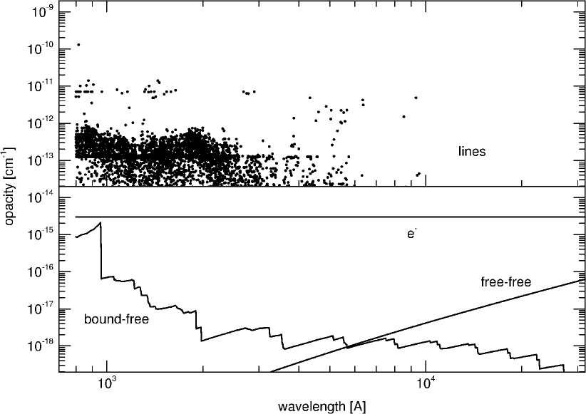
Figure 8: Monochromatic opacity sources at maximum light for a Chandrasekhar mass model of a type Ia supernova from a time-dependent, multi-frequency, LTE calculation. The physical conditions are: $\rho=10^{-13}$ g cm^-3, $T=2.5\times 10^{4}$ K and $t=14$ days. The line opacity shown here is the expansion opacity as given by equation 52 (see text).

Figure 8 displays the various sources of opacity for a mixture of ⁵⁶Ni (20%), ⁵⁶Co (70%), and ⁵⁶Fe (10%), at a density of $10^{-13}$ g cm^-3 and temperature of $2.5\times 10^{4}$ K, typical perhaps of maximum-light in a Chandrasekhar-mass explosion. The excitation and ionization were computed from the Saha-Boltzmann equation. The opacity approximation of Eastman & Pinto (1993–also see below) was used for the line opacity, which greatly exceeds that from electron scattering. Bound-free and bound-bound transitions contribute negligibly to the overall opacity, but they are important contributors to the coupling between the radiation field and the thermal energy of the gas. The opacity is very strongly concentrated in the UV and falls off steeply toward optical wavelengths. As was noted by Montes & Wagoner (1995), the line opacity between 2000 and 4000Å fall off roughly as $d{\rm ln}\kappa_{\lambda}/d{\rm ln}\lambda\sim-10$. It will be shown that the steepness of this decline rate toward the optical has important implications for the effective opacity in SNe Ia and the way in which energy escapes.

Not only is the opacity from lines greater than that of electron scattering, it is also fundamentally different in character from a continuous opacity. In a medium where the opacity varies slowly with wavelength, photons have an exponential distribution of pathlengths. Their progress through an optically thick medium is a random walk with a mean pathlength given by $(\rho\kappa)^{-1}$. In a supersonically expanding medium dominated by line opacity there is a bimodal distribution of pathlengths. The line opacity is concentrated in a finite number of isolated resonance regions. Within these regions, where a photon has Doppler shifted into resonance with a line transition, the mean free path is very small. Outside these regions, the pathlength is determined either by the much smaller continuous opacity or by the distance the photon must travel to have Doppler shifted into resonance with the next transition of longer wavelength. For the physical conditions of Figure 8, the mean free path of the photon goes from approximately $5\times 10^{14}$ cm in the continuum (due to electron scattering) to less than $\sim 10^{6}$ cm when in a line. The usual random-walk description of continuum transport must be modified to take this bimodal distribution into account.

Within a line, a photon scatters on average $N\sim 1/p$ times. $p$ is the Sobolev escape probability per scattering for escape, which is accomplished by Doppler shifting out of resonance. In spite of this possibly large number of scatterings needed for escape, a photon spends only a small fraction of its flight time in resonance with lines. The effect is quite different from that of a similar observer-frame optical depth arising from a continuous opacity.

Because of the very supersonic expansion of the supernova’s ejecta, we can make use of Sobolev theory to describe the path of a photon, following the discussion of Eastman & Pinto (1993). The Sobolev optical depth of a line transition with Einstein coefficient $B_{lu}$ is (ignoring stimulated emission)

$$\tau_{s}={{h}\over{4\pi}}{{n_{l}B_{lu}}\over{|\partial\beta/\partial l}}$$ (44)

where $n_{l}$ is the lower level number density and $\partial\beta/\partial l\sim 1/ct$ is the velocity gradient over the speed of light. The probability of escape from the line transition is

$$p={{1-e^{-\tau_{s}}}\over{\tau_{s}}}.$$ (45)

Castor (1970). Consider a photon which is emitted in resonance at frequency displacement $x$ and subsequently re-absorbed at displacement $x^{\prime}<x$, having travelled a distance $(x-x^{\prime})\Delta\nu_{D}/(\partial\beta/\partial l)$, where $\Delta\nu_{D}$ is the thermal Doppler width. Assume for the moment that the line has a negligible photon destruction probability. We will address thermal destruction below. The optical depth between emission and absorption is

$$\tau(x,x^{\prime})=\tau_{s}\int_{x^{\prime}}^{x}\phi(t)dt,$$ (46)

where $\phi(x)$ is the normalized line absorption profile. The probability that a photon emitted at $x$ will travel a distance $(x-x^{\prime})ct$ to be re-absorbed at $x^{\prime}$ is

$$\tau_{s}\phi(x)\phi(x^{\prime})exp\left\{-\tau(x,x^{\prime})\right\}.$$ (47)

Assuming complete redistribution, the average value of $x-x^{\prime}$ is then

$$<x-x^{\prime}>={{\tau_{s}\int_{-\infty}^{\infty}\phi(x)\int_{-\infty}^{x}(x-x^{\prime})\phi(x^{\prime})exp\left\{-\tau(x,x^{\prime})\right\}dx^{\prime}dx}\over{1-\left(1-e^{-\tau_{s}}\right)/\tau_{s}}}.$$ (48)

Here, the denominator is just the total probability of reabsorption, $1-p$. For a Doppler line profile, this can be approximated as $<\!x-x^{\prime}\!>\sim 0.8/(1+\tau_{s}/5)$ Eastman & Pinto (1993). The typical distance travelled between scatterings in the transition is then

$$\delta r=<\!x-x^{\prime}\!>{{\Delta\nu_{D}}\over{(\partial\beta/\partial l)}}.$$ (49)

For homologous expansion $(\partial\beta/\partial l)=1/ct$. On average, the photon will scatter $N\sim 1/p$ times, and the total distance covered while trapped in the line resonance will be

$$\delta r_{L}=\left(1/p-1\right)\delta r.$$ (50)

In a very optically thick line, the photon will thus travel a distance equal to $4v_{th}/v_{exp}$ times the radius of the ejecta while trapped within a line. Since $v_{th}/v_{exp}<10^{-2}$ at all times, the photon travels a negligible distance, and hence spends a negligible time in resonance with any one line.

What this means is that each time an optically thick line absorbs a photon, the photon is almost instantaneously re-emitted in a random direction. From the point of view of the diffusion of radiation through the ejecta, each line resonance interaction acts like a single scattering event, independent of the optical depth of the transition! The distribution of mean free paths will thus be determined by the continuum opacity and the distribution of lines in energy. In a medium with little continuous opacity the mean free path of a photon is the average distance a photon travels between resonances. The effective mean free path has little to do with any conventionally-defined monochromatic opacity.

For the purpose of estimating the diffusion time, the effective total “optical depth” of the supernova for a photon emitted from the center of the remnant at frequency $\nu$ is the number of lines interactions a photon undergoes in Doppler shifting from $\nu$ to $(1-v_{exp}/c)\nu$. This optical depth may be written as

$$\tau(\nu)=\sum_{\{k|\nu\geq\nu_{k}\geq\nu(1-v_{exp}/c)\}}\left(1-\exp(-\tau_{k})\right)$$ (51)

The sum is over all lines with Sobolev optical depths $\tau_{k}$ and transition frequencies, $\nu_{k}$, lying in the interval $\nu\geq\nu_{k}\geq\nu(1-v_{exp}/c)$.

The evolution of this optical depth with time depends on whether the lines are optically thick or optically thin. In the limit that all lines are optically thick, $\tau_{k}>>1$, $\tau(\nu)$ is just the number of lines in the range $(\nu(1-v_{exp}/c),\nu)$ and, barring significant changes in excitation conditions, is constant with time. In the other extreme, where all lines are optically thin, $\tau_{k}<<1$ and $\tau(\nu)=\sum_{l}\tau_{l}$. Since $\tau_{l}\propto t^{-2}$ (again, barring changes in excitation conditions), $\tau(\nu)\propto t^{-2}$, and behaves like a continuum optical depth which is proportional to the ejecta column density.

We can derive an effective monochromatic opacity coefficient by setting $\rho\kappa(\nu)R_{max}=\tau(\nu)$. This would correspond to a global average over the frequency range $(\nu(1-v_{exp}/c),\nu)$. A more local quantity is obtained by reducing this range to $(\nu,\nu+\Delta\nu)$, where $\Delta\nu\sim\nu\Delta r\partial\beta/\partial r$, giving

$$\kappa(\nu)={\nu\over\rho\Delta\nu}{\partial\beta\over\partial r}\sum_{\{k|\nu\leq\nu_{k}\leq\nu+\Delta\nu)\}}\left(1-\exp(-\tau_{k})\right).$$ (52)

This is the expansion opacity given in Eastman & Pinto (1993). It has the advantage of being a purely local quantity. The expansion opacity formulation of Karp et al. (1977) and its descendents, on the other hand, always averages over a mean free path. This distance can easily become larger than the distance over which the material properties change or even than the supernova itself.

Figure 9: The density of lines in energy space at maximum light (18 days). The histograms are the number of lines in $10^{4}$ km s^-1 to the red of a given wavelength, binned in energy. The heavy line includes all lines with an average (over volume) Sobolev optical depth greater than unity. The two lower histograms show the same quantity, but include lines with average Sobolev optical depth greater than 6.7 and 67. Roughly speaking, the optical depth one curve will decline to resemble the optical depth 6.7 curve at 31 days. Data are taken from the same calculation as for Figure (8). The dotted lines are schematic flux distributions for blackbody radiation fields of one, two, and three $\times 10^{4}$ K for comparison.

In terms of the effective total optical depth, $\tau(\nu)$, the diffusion time can be written $t_{d}\approx\tau(\nu)R(t)/c$. By setting $t_{d}=t$, substituting $R(t)=v_{exp}t$ and $v_{exp}\sim 10^{4}$ km s^-1, one finds that $\tau(\nu)\sim c/v_{exp}\sim 30$. In the UV, $\tau(\nu)>>30$, and since the Sobolev optical depth of many of these lines is $>>1$, $\tau(\nu)$ will remain approximately constant with time. The fact that there is a peak in the light curve, which occurs when $t_{d}=t$, means that the flux mean optical depth must drop below $\sim 30$.

In Figure 9 we show $D(\nu)=$ the density of lines per $10^{4}$ km s^-1, for the same conditions as were used for Figure 8, at 18 days past explosion, with lines taken from the Kurucz line list Kurucz (1991). The uppermost curve is the spectral density of all lines included in the calculation. Below that is all lines with $\tau_{s}>2/3$, and further down are all lines with $\tau_{s}>6.7$ and 67. If we exclude lines for which $\tau_{s}\,\hbox{\raise 1.99997pt\hbox{$<$}\kern-8.00003pt\lower 3.01385pt\hbox{$\sim$}}\,1$, then $D(\nu)\approx\tau(\nu)$. Superimposed upon these curves for reference are three blackbody distributions (the vertical scale is arbitrary). For temperatures above $10^{4}$ K, most photons see a value of $\tau(\nu)$ greatly in excess of the critical value derived above and remain trapped with an ever-increasing diffusion time. Since individual line Sobolev optical depths decline as $1/t^{2}$, it will not be until  50 days when the $2\times 10^{4}$ K Planck mean of $\tau(\nu)$ falls below 30. What, then, accounts for the fact that the light curve peaks at 18 days and not 50 days? One possibility may be, at least in part, that as photons random walk their way out, they are Doppler shifted to longer wavelengths where the effective optical depth is much smaller.

If photons must scatter on order $\tau(\nu)^{2}$ times to escape, and the mean free path is $R/\tau(\nu)$, we can ask what the accumulated Doppler shift might be, following this path. Since, for homologous expansion $dv/dr=v_{max}/R=1/t$, the total Doppler shift is $\tau(\nu)\nu v_{max}/c\sim\nu$, i.e. of order of the entire energy of the photon! This implies that, in the absence of photon destruction mechanisms (electron collisional de-excitation, branching), a photon emitted in the interior will scatter off lines until it has accumulated sufficient redshift to put it at a frequency where $\tau(\nu)$ is small enough to permit escape.

3.2 Photon Collisional Destruction and the Thermalization Length

The discussion of line opacity has so far assumed that lines are coherent scatterers, with no account taken of photon “destruction”. By this we mean any alternative channel for de-populating the upper state other than emission and escape of a photon in the original transition. The two most important mechanisms for this are branching and collisional depopulation by thermal electron collisions.

Figure 10: The opacity of a gas at the same conditions as in Figure 8, decomposed into thermal destruction (top: equation 55), photon splitting (middle: equation 57), and coherent scattering (bottom: equation 58). LTE level populations were employed.

We first examine the efficiency for collisional destruction, that upon being excited to the upper level of the transition, the absorbing atom is collisionally de-populated and the photon’s energy is added to (or subtracted from) the thermal kinetic energy of the gas. The collisional destruction probability per line interaction to upper level $u$ (not per single scattering) can be written

$$\epsilon_{u}={{n_{e}\sum_{l}C_{ul}}\over{n_{e}\sum_{l}C_{ul}+\sum_{l}p_{ul}A_{ul}}}$$ (53)

where, for $E_{u}>E_{l}$

$$n_{e}C_{ul}={8.629\times 10^{-6}\Omega_{ul}(T)n_{e}\over g_{u}\sqrt{T}}$$ (54)

(cf. Osterbrock89) is the rate per atom of collisions from state $u$, with statistical weight $g_{u}$, and $p_{ul}A_{ul}$ is the effective radiative de-excitation rate. To investigate the effect of electron collisions on the effective line opacity one can use equation 52, with each line $k$ weighted by the probability for thermalization:

$$\kappa_{thm}(\nu)={\nu\over\rho\Delta\nu}{\partial\beta\over\partial r}\sum_{\{k|\nu\leq\nu_{k}\leq\nu+\Delta\nu\}}\left(1-\exp(-\tau_{k})\right)\times\epsilon_{k}$$ (55)

where $\epsilon_{k}$ is the thermalization probability for line $k$ (equation 53) and $\Delta\nu$ is the frequency bin size. The top panel of Figure 10 shows $\kappa_{thm}$ for the same line list and conditions as in Figure 8. Van Regemorter’s formula Van Regemorter (1962) was used to calculate the collision rates, $\Omega_{ul}$ but in no case was the resulting collision strength allowed to be less than unity. For this particular example, $\kappa_{thm}$ peaks at a value of $\sim 10^{-4}\ \hbox{cm}^{2}$ near 1500 Å. To put this in context we must consider the question of what value of $\kappa_{thm}$ is sufficient to bring the gas and radiation field into thermal equilibrium. This will occur when $\tau_{thm}\equiv\rho R_{max}\sqrt{\kappa\kappa_{thm}}\,\hbox{\raise 1.99997pt\hbox{$>$}\kern-8.00003pt\lower 3.01385pt\hbox{$\sim$}}\,1$, where $\kappa$ is the total opacity. For a 1.4 M_⊙ uniform density sphere expanding at $10^{9}$ km s^-1, the column density at 18 days is $\rho R_{max}\sim 276$ g cm^-2. At 1500 Å, $\kappa_{thm}\sim 10^{-4}$ cm² g^-1, while the total opacity is $\kappa\sim 1$ cm² g^-1, so $\tau_{thm}\sim 2.8$ —barely adequate to thermalize the radiation field to the local gas temperature. Longward of 1500 Å the situation is somewhat different. At 3000 Å, for instance, $\kappa\sim 10^{-3.5}$ and $\kappa_{thm}\sim 10^{-6}$, so $\tau_{thm}\sim 5\times 10^{-3}$—much less than 1 and entirely insufficient for thermalization.

While these numbers should be taken as no more than order of magnitude estimates, they are accurate enough for us to conclude that near maximum light, the electron density in Type Ia supernova ejecta is too low for collisional destruction to bring about thermalization between gas and the radiation field, at least at wavelengths $\lambda\,\hbox{\raise 1.99997pt\hbox{$>$}\kern-8.00003pt\lower 3.01385pt\hbox{$\sim$}}\,2000$ Å. We expect therefore that the radiation field at longer wavelengths may be significantly different from a Planck function at the local gas temperature. This is a very important point. It means that there is no depth in the supernova to apply the usual, equilibrium radiative diffusion inner boundary condition wherein it is assumed that $J(\nu)=B(\nu,T_{gas})$. We show below that line scattering results in a pseudo-continuous spectrum, however this must not be confused with a continuum that arises from thermalization mediated by electron collisions.

3.3 Photon Splitting and Enhanced Escape

Another possible fate for a photon trapped in a line resonance is that it will decay from the upper level, not in the transition it was absorbed in, but to some other state of lower energy. The probability that a photon trapped in a resonance with upper state $u$ will be escape the resonance region in via downward transition $l$, is given by the branching ratio

$$b_{ul}={{p_{l}A_{l}}\over{n_{e}\sum_{j}C_{j}+\sum_{k}p_{k}A_{k}}}$$ (56)

where the sum $k$ is over all lines with the same upper level $u$, including line $l$. While UV lines tend to have the highest Einstein $A$ values (for dipole permitted transitions $A\propto\lambda^{-2}$) they also tend to arise from levels nearest the ground level, to have higher optical depths and, therefore, smaller escape probabilities. This may lead to a larger probability of decay into another, longer wavelength transition, and further cascade into yet other transitions. Let us call this process “photon splitting”, as the effect is to split a photon’s energy up into a series of longer-wavelength photons. This process is well observed in nebulæ, where each photon of higher-energy transitions in the Lyman series of hydrogen is “degraded” to emerge from the lowest-energy transitions in lower-energy series. The energy in Lyman-$\gamma$ photons, for example, is “split” into Lyman-$\alpha$, Balmer-$\alpha$, and Bracket-$\alpha$ photons. While the inverse process, absorption from a high-lying state and decay into a higher-energy transition, can and does occur, it must do so less frequently by obvious thermodynamic considerations (Rossleand’s Theorem of Cycles—cf. Mihalas78). Pinto (1988) noted the importance of splitting to spectrum formation in SNe Ia in the nebular phase. Li & McCray (1996) showed that it is an important effect in SN 1987A at late times as well.

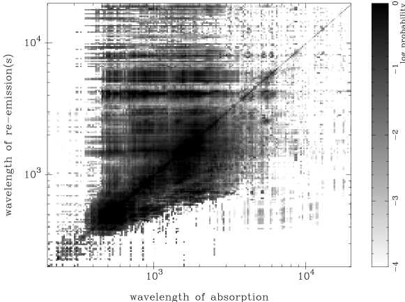
Figure 11: The cascade matrix for a photon absorbed into a transition with wavelength given by the abscissa and emitted into (possibly many) wavelengths given by the ordinate. The intensity represents the the probability of branching multiplied by the probability of being trapped in the absorbing transition. Thus, absorptions at low optical depth, which may nonetheless lead most likely to multiple splittings, are suppressed. The line list and physical conditions are again the same as for Figure 8.

In Figure 11 we show the relative probability that a photon’s energy, absorbed into a transition at a given wavelength, is re-emitted at one or more other wavelengths, weighted by the probability of absorption into the initial transition. It is much like the more familiar recombination cascade matrix, but instead of a collisional process pumping the high energy states, in this case it is line absorption. There is a considerable tendency for energy absorbed in the UV to come out in the optical and infrared. This tendency is enhanced by the radiative transfer through the ejecta, as a photon emitted in the UV is overwhelmingly likely to be re-absorbed in another thick transition and given another opportunity to split, while those photons emitted at longer wavelengths are more likely to escape.

In addition, the rate of electron collisions coupling states of similar energies is much larger than those which remove a substantial fraction of the photon’s energy to the gas. These collisions between states of similar energies have the effect of opening up an even larger number of subordinate transitions, enhancing the rate of “splitting”.

As was done for electron collisional destruction, we can define an effective line opacity for splitting as

$$\kappa_{spl}(\nu)={\nu\over\rho\Delta\nu}{\partial\beta\over\partial r}\sum_{\{k|\nu\leq\nu_{k}\leq\nu+\Delta\nu)\}}\left(1-\exp(-\tau_{k})\right)\times\sum_{l\neq k}b_{u(k)l}$$ (57)

where $b_{u(k)l}$ is as given by equation 56 and $u(k)=$ the upper level of transition $k$. The sum is over all downward transitions except $l$. We can similarly define an effective scattering opacity as the line opacity multiplied by the probability that a photon absorbed into a transition ultimately escapes as a single photon at the same energy:

$$\kappa_{scat}(\nu)={\nu\over\rho\Delta\nu}{\partial\beta\over\partial r}\sum_{\{k|\nu\leq\nu_{k}\leq\nu+\Delta\nu)\}}\left(1-\exp(-\tau_{k})\right)b_{u(k)k}$$ (58)

Examples of $\kappa_{spl}(\nu)$ and $\kappa_{scat}(\nu)$ are shown in the middle and bottom panels of Figure 10, respectively.

With the exception of a few optical wavelengths where $\kappa_{thm}$ dominates, the bulk of the line opacity may be described as primarily “splitting” and “scattering”. This then provides another path for energy to escape from the supernova. Even deep within the ejecta where the UV optical depth is quite great, there is a significant “leak” of energy downward in frequency to energies where the optical depth is much lower. Splitting is a much more efficient mechanism for downgrading photons in energy than the Doppler shift accumulated through repeated scatterings described in the previous section.

Figure 12: Photons with a Planck distribution in energy and at three different temperatures were emitted uniformly throughout the volume of a constant density sphere and followed by a Monte Carlo simulation until emergence. The model has an outer velocity of $10^{9}$ km s^-1 and total, pure-scattering optical depth of $\tau_{e}=10$.

It is instructive to examine the results of a few simple, schematic models. In these, the supernova is taken to be a constant-density sphere expanding homologously with an outer velocity of $10^{4}$ km s^-1. Photons are emitted uniformly throughout the volume of this sphere with a Planckian energy distribution. While emitting the photons at the center of the sphere (and hence at a larger average optical depth) would have provided more extreme demonstrations of the scattering physics, uniform emission is closer to the case in a real supernova. The fate of a large number of emitted photons is followed with a simple Monte Carlo procedure.

The first calculation illustrates the progressive redshift of trapped radiation which results from multiple scatterings. The opacity is due only to scattering coherent in the co-moving frame. The total optical depth of the “supernova” is 10. This corresponds to the electron opacity of a Chandrasekhar mass with an outer velocity of $10^{4}$ km s^-1 at 15 days past explosion, ionized on average to Co V. In this calculation a typical photon looses 8% of its energy before escaping.

Figure 13: An initially Planckian radiation field at three different temperatures (dotted lines) were transported through the line opacity described in the text. The total injected energy is the same in each case, and the emergent spectra (histograms) are virtually identical.

In the next calculations we have used a picket-fence opacity with a line density $D(\lambda)$ which is a smooth power-law approximation to that shown in Figure 9:

$$D(\lambda)=\left\{\begin{array}[]{ll}400&\lambda<1500\\ 10^{3}(\lambda/1500)^{-4.5}&\lambda>1500\end{array}\right.$$ (59)

All of the lines have a Sobolev optical depth of 10 (consequently, $\tau(\lambda)=D(\lambda)$), although the result is unchanged with any value of the line optical depth greater than unity. Upon absorbing a photon, a line has a given probability $\sigma$ of splitting into a pair of photons with longer wavelengths. Energy is conserved by requiring that the combined photon energies equals that of the absorbed photon. This is a far more random splitting than that imposed by a real set of atomic data where each line has a fixed set of branching ratios into a finite (though typically quite large) number of wavelengths. It nonetheless captures the spirit of the photon splitting process described above and is computationally expedient. In these calculations we have ignored electron collisional destruction.

In Figure 13 we have taken the splitting probability to be $\sigma=0.25$ and computed three spectra corresponding to emission temperatures of $1,2,$ and $3\times 10^{4}$ K, but in each case with the same total emission rate. The result of this calculation is remarkably different in character from the coherent scattering case. One can see from the figure that as long as the peak wavelength of the blackbody emission spectrum, $\lambda_{Wien}$, lies at a wavelength characterized by $\tau(\lambda_{Wien})>>1$, the shape of the emitted flux is identical in all cases; any memory of the shape of the thermal emission spectrum has been lost.

Figure 14: Photons from the blackbody shown by the dotted line were scattered through the line opacity described in the text. While the shape of the emergent spectrum (histograms) is sensitive to the splitting probability $\sigma$, it is independent of the input blackbody’s temperature. The solid lines following the histograms are blackbodies at 4500, 5500, and 7500 K.

Figure 14 shows the effect on the emergent spectrum of varying the splitting probability. We have chosen three values – 0.25, 0.1, and 0.025 – and a single emission spectrum at $2\times 10^{4}$ K. In all three cases the emergent spectrum is completely insensitive to the temperature of the emission spectrum (as established by calculations similar to those of Figure 13). However, it is quite sensitive to the splitting probability $\sigma$. A remarkable feature of these calculations is that the emergent spectrum comes very close in shape to a Planck spectrum. The solid lines in the figure which follow the emergent spectra are blackbodies at temperatures of 4500, 5500, and 7500 K. In detail, the emergent flux has a Rayleigh-Jeans tail and a Wein cutoff, and is just slightly more peaked than an actual blackbody; they have a small, but non-zero, chemical potential. The peak wavelength, $\lambda_{peak}$, is determined by the condition $\sigma\tau^{2}(\lambda_{peak})\sim 1$. Any departure in the spectral shape from an exact Planck function would most likely be impossible to discern in spectra of real supernovae as the pseudo-continuum produced by multiple line splittings has superimposed upon it a number of strong lines as well as structure from deviations in $D(\lambda)$ from the smooth power-law employed for these examples.

The fact that one can use the basic physical picture these examples outline to produce a spectrum which is nearly a Planck function in shape but which has nothing to do with the “thermal emission” leads one to suspect that observed color temperatures may have less to do with close thermal coupling between gas and radiation field and more to do the distribution of lines and branching ratios in the complex atomic physics of the iron group.

The physical process underlying the production of these pseudo-blackbodies is simple: the energy in short wavelength photons is continuously redistributed to longer wavelengths until an equilibrium is reached between the injection of energy and its loss from the system. The similarity to equilibrium thermodynamics suggests an interesting possibility. If the redistribution in energy from multiple splittings is sufficiently large and random to reach a thermodynamic limit, perhaps a calculation which assumes this thermodynamic limit might not be too much in error. The occupation numbers of the atomic states in the scattering system might not be too far from their LTE values. In this case, treating the lines as pure absorbers and using LTE level populations might not be a bad approximation. The approach to this thermodynamic limit is fundamentally different, however. In a gas, the distribution of particles in phase space approaches a Maxwellian distribution because of the essentially infinite number of ways collisions can redistribute momentum. In the usual LTE radiation transport picture, either a large bound-free continuum optical depth or the dominance of collisional rates over radiative ones ensures that the thermodynamic equilibrium established by gas particles is strongly coupled to the radiation field, giving it an equilibrium distribution as well. This is in spite of the relatively restricted possibilities for energy redistribution in the photon gas through radiative processes. In the present case, the extreme complexity of the radiative processes allows the photon gas to reach something of a thermodynamic equilibrium on its own. This equilibrium will then drive the level populations to LTE values through radiative processes. We may expect, then, that the electron gas will be driven toward a similar equilibrium state through its (albeit weak) coupling to the photon gas. In a less schematic calculation, of course, the emergent spectrum would reflect the gaps and bumps of Figure 9, and the result would be a line spectrum similar in character to that emitted by a supernova. The important point is that the shape of the emergent spectrum reflects the variation in $D$ and not the underlying radiation temperature.

Several sources of uncertainty exist regarding the line-blanketing opacity. One involves the atomic data. The line list most commonly employed is that of Kurucz (1991). Because the number of lines which contribute to the total opacity is so large, numbering in the hundreds of thousands or more, there is no way at present to know either how accurate nor how complete the list is with respect to the weaker lines. The bulk of the opacity comes from the cumulative effect Harkness (1991) of many weak lines of iron group elements and the lack of any information about completeness in the data set must be regarded as an unknown source of uncertainty in the calculations.

Another uncertainty in the line-blanketing opacity arises from approximations in its numerical representation. It has been noted by several authors (e.g. Hoflich95 and BaronHM96) that the Sobolev theory, developed for isolated lines, is in error when lines populate wavelength space so densely that there is significant overlap of the intrinsic line profiles in the co-moving frame. While there have been no detailed studies of the magnitude of this error in the present context, such an error undoubtedly occurs to some extent. Unfortunately, the very great number of lines which the above discussion shows must be included in a calculation makes a Sobolev treatment the only viable one with present technology. An “exact” numerical treatment approaching the accuracy of Sobolev theory would require several tens of frequency points per line. Even allowing for significant overlap, this implies a number of frequency grid points at least several times the number of lines—at the very least, several million points. There are at present no numerical techniques up to the task of representing the frequency variation of the opacity with unambiguously sufficient resolution. Eastman & Pinto (1993) compared supernova spectra calculated with and without the Sobolev approximation and found minimal differences. Thus, while the objection is correct in principle, it is rendered moot in current practice.

There is another indication that such a scattering-mediated “thermalization” may be taking place in SNe Ia. Höflich et al. (1995) and Baron et al. (1996) note that the agreement of their calculated maximum-light spectra with observations is significantly improved by the inclusion of additional thermalization. They have attributed this to a lack of accurate collision cross sections. Under this assumption, they empirically fit an enhancement to the collision rates they employ, using the agreement of their simulations with observed spectra as a criterion. This may well be an appropriate exercise. On the other hand, the approximations they employ to determine collision rates (the same as we have employed above) work well on average in other astrophysical and terrestrial applications; in particular, there is no reason to suspect that these approximations are systematically incorrect other than the disagreement of computed supernova spectra with observations. The additional thermalization resulting from splitting in a sufficiently large number of lines may be another, less artificial, way to achieve this same effect.

3.4 Frequency-Integrated Mean Opacities

Simple analytic light curve models such as the one presented in section 2 and most, if not all, radiation hydrodynamic calculations of Type Ia supernovae performed to date, rely upon the existence of a well-defined, frequency-integrated mean opacity. A natural choice for this mean opacity is the Rosseland mean, which has a long history of use in astrophysical contexts. The formally correct choice is, of course, the flux mean, but the whole point of using a mean opacity is to avoid the multi-group calculation of the flux which is essential to the computation of the flux mean in the first place! In this section we use the results of multi-group radiation transport calculations to compare the Rosseland mean and flux mean opacities near maximum light in the delayed-detonation model DD4 of Woosley & Weaver (1994).

The second monochromatic radiation transport moment equation may be written as

$${1\over{c^{2}}}{{DF_{\nu}}\over{Dt}}+{{\partial P_{\nu}}\over{\partial r}}+{{3P_{\nu}-E_{\nu}}\over r}+{2\over c^{2}}{v\over r}\left(F_{\nu}+4\pi N_{\nu}\right)+$$

$${1\over c^{2}}{\partial v\over\partial r}\left(2F_{\nu}-4\pi N_{\nu}\right)-{\partial\over\partial\ln\nu}\left({v\over r}F_{\nu}+\left({\partial v\over\partial r}-{v\over r}\right)4\pi N_{\nu}\right)=-{1\over c}\rho\kappa_{\nu}F_{\nu}$$ (60)

where $N_{\nu}$ is the third moment of the radiation field specific intensity. If this equation, as written, is integrated over frequency, one obtains equation 2. The right hand side of equation 2 can be written as $-\rho\kappa_{F}F/c$, where the flux mean opacity, $\kappa_{F}$, is defined as

$$\kappa_{F}\equiv F^{-1}\int_{0}^{\infty}\kappa_{\nu}F_{\nu}\,d\nu$$ (61)

This is clearly the correct quantity to use for the mean opacity. The problem, as mentioned above, is that the calculation of the flux mean requires prior knowledge of $F_{\nu}$ and thus requires solution of the frequency-dependent problem. On the other hand, having calculated $F_{\nu}$ by some much more complex calculation for a variety of models, we can try to discover regularities in the behavior of $\kappa_{F}$ which may be useful in more approximate calculations.

At large enough optical depth ($\tau_{thm}>>1$) the gas and radiation field will be thermalized and $E_{\nu}\approx 4\pi B_{\nu}(T)$. The radiation field will be isotropic, so that $P_{\nu}\approx E_{\nu}/3$. The expansion is homologous so $v/r=\partial v/\partial r=1/t$. Finally, since $\rho\kappa_{\nu}ct>>1$, the time derivative term in equation 60, $c^{-2}DF_{\nu}/Dt$, may be set to zero. Substituting these relations into equation 60 gives

$${\partial F_{\nu}\over\partial\ln\nu}-(3+\rho\kappa_{\nu}ct)F_{\nu}={4\pi ct\over 3}{\partial T\over\partial r}{\partial B_{\nu}(T)\over\partial T}$$ (62)

where we have written $\partial B_{\nu}(T)/\partial r=\partial B_{\nu}(T)/\partial T\times\partial T/\partial r$. This equation is straightforward to solve:

$$F_{\nu}=-{4\pi ct\over 3}{\partial T\over\partial r}\int_{\nu}^{\infty}{\partial B_{\nu^{\prime}}(T)\over\partial T}\left({\nu\over{\nu^{\prime}}}\right)^{3}\exp\left(-ct\int_{\nu}^{\nu^{\prime}}{\nu^{\prime\prime}}^{-1}\rho\kappa_{\nu^{\prime\prime}}\,d{\nu^{\prime\prime}}\right){\nu^{\prime}}^{-1}\,d{\nu^{\prime}}$$ (63)

The Rosseland mean opacity can now be determined from the definition

$$F={-4\pi\over 3\rho\kappa_{R}}{\partial T\over\partial r}\int_{0}^{\infty}{\partial B_{\nu}(T)\over\partial T}\,d\nu.$$ (64)

Integrating equation 63 over $\nu$ and combining with equation 64 gives

$$\kappa_{R}={\rho\pi t\over aT^{3}}\int_{0}^{\infty}d\nu\int_{\nu}^{\infty}{\partial B_{\nu^{\prime}}(T)\over\partial T}\left({\nu\over{\nu^{\prime}}}\right)^{3}\exp\left(-ct\int_{\nu}^{\nu^{\prime}}{\nu^{\prime\prime}}^{-1}\rho\kappa_{\nu^{\prime\prime}}\,d{\nu^{\prime\prime}}\right){\nu^{\prime}}^{-1}\,d{\nu^{\prime}}.$$ (65)

Note that we have used a large number of approximations to derive this expression: a large optical depth, a thermalized radiation field, and a weak time dependence of the radiation field. The most important of these is that the radiation field be thermalized. We have shown above that we do not expect this to be the case; we demonstrate in the following that the radiation field is in fact not thermalized.

We have undertaken a series of light curve calculations with a more modern version of the code EDDINGTON described in Eastman & Pinto (1993). Here we present the result of just one such calculation—Paper II will contain a more systematic examination of the light curves predicted for a variety of SNe Ia models.

Since our purpose was to make illustrative calculations and not to model any individual supernova, the size of the calculations was kept small enough to run on a workstation in reasonable time. Thus, we have assumed LTE and employed a frequency grid with 3500 points from 33Å to $45\mu$, using the monochromatic opacity approximation given by equation 52 to represent all but the strongest 3000 lines in the spectrum.

In EDDINGTON, the gas temperature is determined by solving the time-dependent first law of thermodynamics. Heating is from radiative absorption, fast particles from Compton scattering of gamma-rays, and decay positrons. Losses are from expansion and radiative emission. Near peak, because the energy density is dominated by radiation the same gas temperature would be obtained by balancing heating and cooling and ignoring the gas pressure contribution to $PdV$ losses; clearly, however, the $PdV$ work done by the radiation must still be included. The local energy deposition from radioactive decay is determined with reasonable accuracy, especially before 50 days, by doing a separate deterministic transport calculation for each $\gamma$-ray line emitted in the decay cascade from ⁵⁶Ni through ⁵⁶Fe as described in Woosley et al. (1994). Energy from ⁵⁶Co positrons, irrelevant to the light curve near peak, was deposited in situ. Blinnikov et al. (1996) obtain excellent agreement in results on test problems run with EDDINGTON and with the multi-group implicit radiation-hydrodynamics code STELLA (BlinnikovB93, BartunovBPT94) when the same approximations are used in both codes for the line opacity.

Because the probability of photon destruction from “line splitting” is so large, the best that an LTE calculation can do to represent this inherently non-LTE effect is to redistribute the photon energies thermally. Thus the line opacity of the 3000 strongest lines was taken to be purely absorptive. The opacity from the remaining $3\times 10^{5}$ lines treated by the opacity approximation of Eastman & Pinto (1993) was taken to be purely scattering. While this is a crude approximation to the photon destruction described above, it is the best one can do without performing an extensive time-dependent NLTE calculation, one that is beyond reach of present computing resources.

Figure 15: B and V band light curves of delayed detonation Model DD4 of Woosley & Weaver (1991), calculated as described in the text, compared with data from SN 1991T and SN 1992bc (data from Hamuyetal96). The solid line was calculated from the model with population II primordial abundances, the dotted line with population I. The population I model, though too blue in $B-V$, gives the observed bolometric risetime of $\sim 19$ days, while the bolometric light curve of the population II model rises too quickly, in 15 days.

Figure 15 shows the B and V band light curves of model DD4, as computed by this LTE prescription, compared with data from observations of SNe 1991T and 1991bc. While not an exact reproduction of either object, the fit is relatively good in B and V. In both cases we have taken the basic explosion model, computed from a pure C/O white dwarf, and added population II ($10^{-2}\times$ solar) and population I (solar) abundances. For the population II model, the bolometric curve reaches maximum in only 15 days. The population I model, however, reproduces the observed bolometric risetime of 18 days Vacca & Leibundgut (1996b), though it gives a somewhat worse fit to the observations in V. These curves are remarkable as they are the first models of SNe Ia light curves which peak as late as supernovæ are observed to do (c.f. HoflichKW95). For the first sixty days, the agreement with observation is reasonably good. After this, the supernovæ are observed to make a transition to a quasi-nebular, emission-line spectrum, one which bears little resemblance to a blackbody at any temperature. An LTE calculation would not be expected to be a reasonable representation of the dominant physics; we suspect that any agreement from this model at such a late stage is therefore entirely fortuitous.

Figure 16: Comparison of flux mean ($\kappa_{F}$), Rosseland mean ($\kappa_{R}$) and electron scattering ($\kappa_{e}$) mass opacity coefficients in Model DD4 versus Lagrangian mass coordinate at three times before and after bolometric maximum. Also shown is the ratio of the frequency integrated radiation field mean intensity to the Planck energy density at the local gas temperature ($J/B$). Where $J/B<1$, the gas and radiation field are not in equilibrium.

Figure 16 displays the run of $\kappa_{F}$, $\kappa_{R}$ and $\kappa_{e}$ (the electron scattering mass opacity coefficient), at three different times after explosion. At all times the flux mean opacity is substantially greater than the Rosseland mean, by as much as a factor of 10 near maximum light. The effect this would have on the computed bolometric light curve is comparable to a factor of three change in the total mass of the star (when $E/M$ is held constant)! We have found similar results comparing $\kappa_{F}$ and $\kappa_{R}$ from calculations of other explosion models.

The reason that $\kappa_{F}$ is so different from $\kappa_{R}$ is explained in part by the steep frequency dependence of the line opacity at UV wavelengths ($d\ln\kappa_{\nu}/d\ln\nu\sim 10$). Photon transport takes place out on the Rayleigh-Jeans tail of the Planck spectrum, and the steep frequency dependence of $\kappa_{\nu}$ means that the mean opacity is very sensitive to that long wavelength slope.

In light of the discussion in section 3.2 we would expect $F_{\nu}$ to be different than the diffusion flux given by equation 63. However, for the above calculation we assumed that the strongest lines were purely absorptive. This should have the effect of increasing the thermalization optical depth, driving the radiation field and gas into thermalization, and therefore making the flux and Rosseland mean opacities more equal in value. With a more realistic NLTE treatment of the line opacity, therefore, we would expect an even larger discrepancy between $\kappa_{F}$ and $\kappa_{R}$.

Even at maximum light the departure from radiative equilibrium can be significant. Also shown in Figure 16 $J/B=$ the ratio of the frequency integrated mean intensity to $acT^{4}/4\pi$. At maximum light the criterion that the radiation field be thermalized, required in the derivation of the Rosseland mean opacity, is violated. Where $J/B<1$, the color of the radiation field is hotter than a blackbody at the same energy density. The Rossleand mean, which is weighted by $\partial B_{\nu}/\partial T$ at the local gas temperature, samples the opacity at longer wavelengths than does the flux mean. Because the opacity falls off so strongly with increasing wavelength, the resulting Rosseland mean is lower than the flux mean.

We can understand the variation of the mass opacity coefficients in Figure 16 as a combination of several effects. From the discussion above, we expect the extinction coefficient to be nearly constant with radius, given roughly by the spectral density of lines at some typical energy. As the density drops with radius, we expect the mass opacity coefficient to rise proportionately. At ten days past maximum, for example, the factor of three rise in $\kappa_{F}$ in going from 0.5 M_⊙ to 1.0 M_⊙ is due almost entirely to the density dropping by the same factor. The constancy of $\kappa_{F}$ in the central panel thus implies that the extinction coefficient has fallen by about a factor of three in the same range. Because the flux mean photospheric radius has by this time receded to $\sim 0.68$ M_⊙, this change has little effect upon the luminosity.

The drop toward the center in the first panel is due to the higher ionization of the iron group there. In the inner 0.3M_⊙, the typical ionization stages are Co VII and VIII, while outside of this the typical ions are Co V and VI. The higher ionization stages possess fewer strong transitions in the near UV, so that the spectral density of lines, and hence the extinction coefficient, is smaller.

The smaller change in $\kappa_{R}$ with radius is due to the fact that as one moves out, the temperature drops. This leads to a longer effective wavelength in the weighting function $\partial B_{\nu}/\partial T$, where the monochromatic opacity is lower, and a lower extinction coefficient. Since the density is dropping as well, this leads to a smaller variation in $\kappa_{R}$.

It is interesting to note that if a constant opacity roughly equal to the Rosseland mean in the top panel is used in a grey solution of the transport equations, the bolometric light curve peaks at $\sim 12$ days, not very different from the rise-times found by Höflich et al. (1995) for similar explosion models, employing a Rosseland mean opacity.

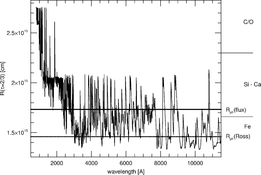
Figure 17: This figure shows the photospheric radius as measured in the observer frame at disk center for Model DD4 at 14 days after explosion, versus wavelength.

Figure 17 displays the photospheric radius ($\tau=2/3$ surface) as a function of wavelength as measured in the observer frame at the center of the disk, 14 days after explosion, with population II primordial abundances. The photosphere is a very strong function of wavelength whose behavior is dominated in the optical by a considerable number of strong lines. Also shown are the Rosseland and flux mean photospheric radii. Clearly, choosing either one as the photosphere and assuming the emergent flux is a blackbody at some temperature is a rather poor representation of the actual behavior. It is interesting to note, however, that the flux mean photosphere at this time lies at the outer extent of the iron-rich region as one would expect from the lack of strong iron lines in the maximum-light spectrum.

It is worth commenting that, whereas the assumption of constant $\kappa$ made in Section 2 in the derivation of the analytic light curve model may at first seem naïve, the results of the multi-group calculations (Figure 16) show that it is, in fact, not such a bad approximation, especially if a constant-density explosion model is employed in the analytic treatment (it is actually $\rho\kappa$ which is constant). This is fortunate, as it gives us confidence that the simple light curve model described above gives a fair representation of the response to changes in various parameters of the explosion model.

4 Time Dependence

As a final, more technical issue, we can use the analytic solution we have developed to examine the validity of various approximations to the solution of the radiative transfer problem in supernovæ. While it may seem obvious that SNe Ia are not steady state phenomena, several papers have appeared in the literature in which the absolute luminosity of some SNe Ia have been estimated ignoring the basic time dependence of the transport physics. This is a natural and indeed necessary assumption for the calculation of NLTE maximum-light spectra, as general, time dependent, NLTE calculations are beyond current computational capabilities at present. It is, however, important to understand the magnitude of the errors which may be incurred by such approximations.

Among the most important and commonly-used approximations is that of steady state—that one or more of the time-dependent terms in equations 1 and 2 can be ignored. These are enormously attractive approximations as they greatly reduce the computational complexity. A time independent problem is much easier to solve than a time dependent one!

Steady-state amounts to the assertion that heating by energy deposition and cooling by radiative processes (and perhaps by expansion as well) are balanced at all times. There are two versions of this approximation. The first asserts that the Lagrangian derivative (the first term in equation 1), is small compared with the flux divergence. In this approximation, the supernova is no different than a static stellar atmosphere. The second (employed, for example, by NugentBHB95 and references therein), takes into account energy loss from $PdV$ work but asserts that the Eulerian derivative $\partial E/\partial t$ is negligible.

Figure 18: The ratios of various terms in the transfer equation as functions of time. Because a logarithmic scale is used, the absolute value of each curve is plotted. Thus, at maximum (near 15 days) the Eulerian derivative changes sign from positive to negative.

In Figure 18 we present ratios of various terms in the transfer equations as functions of time for our fully time dependent solution. For clarity, only the fundamental mode is considered; the inclusion of higher modes will make the time dependence different at different depths in the ejecta but does not alter the character of the solution nor the order of magnitude of the terms.

The ratio of the Lagrangian derivative to the flux divergence in equation 1 is

$${{DE}\over{Dt}}\left[-{1\over{r^{2}}}{{\partial}\over{\partial r}}\left(r^{2}F\right)\right]^{-1}=\psi\left\{-1+{{\tau_{d}}\over{\alpha}}{{\tilde{\epsilon}\theta\Lambda}\over{\phi}}-{{4\tau_{d}}\over{t_{sc}\alpha}}\left(1+t/t_{sc})\right)^{-2}\right\}$$ (66)

Using the asymptotic value equation 36, equation 66 becomes the ratio of the (current) diffusion time to the expansion (elapsed) time and thus goes to zero in the limit of large $t$. At late times, energy is deposited in the ejecta and is immediately radiated away; thus the flux divergence must equal the deposition, and it is appropriate to use a “steady-state” solution which balances instantaneous luminosity against the time varying deposition rate, $\theta(t)\Lambda(t)$.

At peak light, $\dot{\phi}=0$ in equation 34 and in equation 36 as well, so equation 66 becomes the ratio of the present diffusion time to the elapsed time. Since peak occurs when the diffusion time approximately equals the elapsed time, the ratio in equation 66 is $\sim 1$, implying that the time dependent terms cannot be ignored. Thus while steady-state is a fine approximation at late times it is quite a poor approximation at earlier phases of the light curve. Indeed, it is only after 246 days that the ratio in equation 66 falls below 1%.

In the second approximation, what one might call “quasi-steady-state”, only the Eulerian derivative is neglected. We can formulate the ratio of the Eulerian to the advective derivative as

$${{\partial E/\partial t}\over{(v\cdot\nabla)E}}={{t_{sc}}\over{4}}\left[{{\tilde{\epsilon}\theta\Lambda}\over{\phi}}-{{\alpha}\over{\zeta(t)/t_{d}}}\right](1+t/t_{sc})^{2}.$$ (67)

Once again, this ratio goes to zero in the limit of large time, but it also goes to zero at peak, when $\dot{\phi}=0$. That this must be so is obvious from examination of the light curves of the previous sections. Before peak, the luminosity of the supernova is less than the rate at which energy is being deposited in the ejecta, even accounting for losses due to expansion. Shortly after peak, the luminosity is greater than the deposition rate. This means that before peak, a store of energy is being built up in the supernova and therefore that $\partial E/\partial t>0$. After peak, this “excess” energy is radiated away, and the energy loss is greater than the loss due to expansion alone so that $\partial E/\partial t<0$. Since the sign of the Eulerian derivative changes when the supernova traverses peak light, there must be a time near peak at which it is zero. This does not mean that the term can be ignored, however. When the effects of all modes are included, the time at which $\partial E/\partial t=0$ is different for each radius. As well, the derivative’s value is changing rapidly; one can see from the figure that only a few days before and after maximum it is 30% as great in magnitude as the advection term.

We wish particularly to draw attention to the erroneous conclusions drawn in this regard by Baron et al. (1996). In that work, its authors express $\partial E/\partial t$ as a finite difference over a time interval $\delta t$. They then go on to show that inclusion of this term has the effect of an additional source or sink of radiation. While this is correct, when comparing the magnitude of various terms they let $\delta t$, which would be the “time step” in a finite difference treatment of the time dependent problem, be the elapsed time. They then conclude that the term is small and can be ignored. This is wrong. While it is obvious that in an implicit difference scheme one approaches some sort of steady state if a sufficiently long time step is employed, it is equally obvious that such a state need have little semblance to a correct solution of the time-dependent equations. This is especially so in that the solution at peak is not an asymptotic limit. If they had chosen a time step small enough to preserve accuracy in the finite difference, $\delta t$ would have been almost two orders of magnitude smaller and their estimate of the relative size of the Eulerian derivative would have been much the same as that determined here.

To see the error in the quasi-steady state approximation another way, consider the limiting case of infinite opacity, radiative equilibrium, and homologous expansion. Equations 1 and 2 then become

$${{DE}\over{Dt}}=-{{4\dot{R}}\over{R}}E.$$ (68)

If we solve this equation directly, we find the expected result that $E\propto t^{-4}$. This clearly contradicts the notion that the intrinsic time derivative of $E$ is zero! In yet another demonstration, if we consider the case in which we set $\dot{\phi}=0$, the light curve must decline monotonically, following the energy deposition. Thus the mere fact that the light curve is observed to peak is testament to the error of the quasi-steady-state.

Perhaps the simplest way to gauge the effects of time dependence upon the light curve is to examine when the luminosity emitted at a given time was deposited in the ejecta. Figure 19 shows the cumulative fraction of luminosity at maximum light as a function of deposition time for a typical supernova model. It is clear that the “residence time” of the energy which emerges from a supernova near maximum light is significant. From the figure, for example, 50% of the luminosity is energy deposited at times earlier than 75% the age of the supernova.

Figure 19: The fraction of maximum light luminosity arising from energy deposited before the time indicated on the abscissa.

Energy is stored predominantly in the form of photons diffusing out through the ejecta. Even the tactic of taking the thermal structure of the matter from a light curve calculation, placing it in an atmosphere code, and calculating the resulting spectrum does not do justice to the presence of these “old photons”. There is no reason to suspect that the radiation temperature is the same as the matter temperature and thus without taking some measure of the radiation field energy density from the light curve calculation there is no way to characterize the spectrum or intensity of these photons in the spectrum calculation. The only way to avoid a serious omission in the physics of spectrum formation is to provide some measure of the spectral shape and intensity of the “old photons” to the atmosphere code. In practice, this means that the spectrum formation problem is the light curve problem; one cannot avoid the inherent time-dependence in calculating either light curves or spectra. Especially when attempting to calibrate SNe Ia as cosmological distance indicators, it is necessary to include all of these important physical effects.

It is true, however, that $\partial E/\partial t$ becomes small near maximum light, and it may be true, despite the presence of “old photons”, that a “quasi-steady-state” treatment may not be too much in error at this epoch. Without a benchmark time-dependent NLTE calculation with which to compare, however, it is difficult to assess the magnitude of any error in the resulting luminosity. Since the spectrum-forming layers of the outer atmosphere are primarily scattering, and since the shape of the pseudo-continuum may have little to do with the gas temperature or the luminosity as demonstrated above, a good agreement with the observed spectrum shape may not in fact imply a reliable estimate of the luminosity.

5 Conclusions

Radiation transport in SNe Ia has long been recognized to be fundamentally different in character from that in other astrophysical objects, a situation arising from the coincidence of large heavy element abundances with a large velocity gradient and a diffusion time comparable with the evolution time. The key to understanding this transport is the realization that diffusion downward in frequency is as important to the escape of energy as its diffusion outward in radius. This coincidence arises due to the rapid decline of the spectral density of optically thick lines with increasing wavelength. While the spectral shape of the trapped radiation field is nearly Planckian at temperatures near $2\times 10^{4}$ K, the flux mediating this escape occurs predominantly at much lower energies.

One can ultimately do justice to such a complex process only by performing detailed, time-dependent NLTE computations, those which are probably beyond the present state of the art, or at least present computers. We have demonstrated by more approximate means, however, some of the most important effects. For the present, the key to understanding lightcurve systematics is to provide a simple model for the lightcurve, and the key ingredient in this effort is to determine a mean opacity. The Rosseland mean, so useful in static atmospheres, is significantly misleading in the present context, leading to an incorrect picture of the escape of radiation and serious errors in photospheric radii and temperatures. We have shown that the flux mean as determined by a multi-frequency computation is remarkably constant in radius and with time during the peak phase of the lightcurve. This allows one to make some progress by adopting a narrow range of values for $\kappa_{F}$ in simple, constant-opacity models.

We have derived an analytic solution of the co-moving frame transport equations which closely reproduces the results of more complex numerical solutions. This allows one to examine a number of key features of the lightcurve physics itself and of the observed systematics in SNe Ia data. One result is the demonstration that the lightcurve and spectrum problem is inherently time dependent and cannot be approximated by time-independent calculations before at least 70 days past explosion. Because the spectrum near maximum light is formed by scattering lines atop a pseudo-continuum of line blends, the shape of the spectrum is relatively insensitive to the luminosity. We suspect that any correlation of line widths and velocities with bolometric luminosity arises from differences in the underlying explosions; the demonstration that a given model reproduces the shape of an observed spectrum does not therefore imply that such a model reproduces the luminosity of the observed explosion. Such a correlation thus requires, for now, an independent, observational calibration.

Using the analytic model, we have explored the effect of changes in a variety of parameters on the resulting lightcurve. These include the opacity, explosion energy, ⁵⁶Ni mass and distribution, and total mass. Of these, there is only one parameter which by itself can explain the observed correlation of peak width and luminosity: the total mass. All others, when varied individually, lead to anti-correlations. This does not necessarily imply that the mass of the explosion is the controlling parameter; there may be various combinations of parameters which, when altered in concert, lead to the same behavior. For example, if the opacity can be shown to be a strong function of the ⁵⁶Ni mass then the behavior of models at a single mass may be able to reproduce the PR. The fact that variations in so fundamental a property of the explosion as the total mass can explain the observed behavior is, to say the least, suggestive.

References

- Arnett (1980) Arnett, W. D. 1980, ApJ, 237, 541
- Arnett (1982) Arnett, W. D. 1982, ApJ, 253, 785
- Arnett (1996) Arnett, W. D. 1996, Supernovae and Nucleosynthesis (Cambridge Univeristy Press)
- Barbon et al. (1993) Barbon, R., Benetti, S., Cappellaro, E., Patat, F., & Turatto, M. 1993, Memorie Societa Astronomica Italiana, 64, 1083
- Baron et al. (1996) Baron, E., Hauschildt, P. H., & Mezzacappa, A. 1996, MNRAS, 278, 763
- Bartunov et al. (1994) Bartunov, O. S., Blinnikov, S. I., Pavlyuk, N. N., & Tsvetkov, D. Y. 1994, A&A, 281, L53
- Blinnikov & Bartunov (1993) Blinnikov, S. I., & Bartunov, O. S. 1993, A&A, 273, 106
- Blinnikov et al. (1996) Blinnikov, S. I., Bartunov, O. S., Popolitov, V. A., Eastman, R. G., & Woosley, S. E. 1996, ApJ, in preparation
- Castor (1970) Castor, J. 1970, MNRAS, 149, 111
- Eastman & Pinto (1993) Eastman, R. G., & Pinto, P. A. 1993, ApJ, 412, 731
- Evans et al. (1989) Evans, R., Van Den Bergh, S., & McClure, R. D. 1989, ApJ, 345, 752
- Hamuy et al. (1993) Hamuy, M., et al. 1993, AJ, 106, 2392
- Hamuy et al. (1996) Hamuy, M., Phillips, M. M., Suntzeff, N. B., Schommer, R. A., Maza, J., Smith, R. C., Lira, P., & Avilés, R. 1996, AJ, ”accepted for publication”
- Harkness (1991) Harkness, R. P. 1991, in SN 1987A and Other Supernovae, ed. J. Danziger & K. Kjär (ESO: Garching), 447
- Höflich (1995) Höflich, P. 1995, ApJ, 443, 89
- Höflich et al. (1995) Höflich, P., Khokhlov, A. M., & Wheeler, J. C. 1995, ApJ, 444, 831
- Höflich et al. (1993) Höflich, P., Müller, E., & Khokhlov, A. 1993, å, 268, 570
- Karp et al. (1977) Karp, A. H., Lasher, G., Chan, K. L., & Salpeter, E. E. 1977, ApJ, 214, 161
- Kurucz (1991) Kurucz, R. L. 1991, in Stellar Atmospheres: Beyond Classical Models, ed. L. Crivellari, I. Hubeny, & D. G. Hummer (Kluwer:Dordrecht), 441
- Li & McCray (1996) Li, H., & McCray, R. 1996, ApJ, 456, 370
- Mihalas (1978) Mihalas, D. 1978, Stellar atmospheres /2nd edition/ (San Francisco, W. H. Freeman and Co., 1978. 650 p.)
- Mihalas & Mihalas (1984) Mihalas, D., & Mihalas, B. W. 1984, Radiation Hydrodynamics (Oxford, Oxford University Press, 1984. 718 p.)
- Montes & Wagoner (1995) Montes, M. J., & Wagoner, R. V. 1995, ApJ, 445, 828
- Nomoto et al. (1984) Nomoto, K., Thielemann, F. K., & Yokoi, K. 1984, ApJ, 286, 644
- Nugent et al. (1995) Nugent, P., Baron, E., Hauschildt, P. H., & Branch, D. 1995, ApJ, 441, L33
- Osterbrock (1989) Osterbrock, D. 1989, Astrophysics of Gaseous Nebulæ and Active Galactic Nuclei (University Science Books)
- Phillips (1993) Phillips, M. M. 1993, BAAS, 182, 2907
- Pinto & Eastman (1996) Pinto, P., & Eastman, R. 1996, ApJ, in preparation
- Pinto (1988) Pinto, P. A. 1988, Ph.D. thesis, California Univ., Santa Cruz.
- Pollas (1994) Pollas, C. 1994, in Supernovæ, Les Houches, Session 1990, ed. R. M. S. Bludman & J. Zinn-Justin (North-Holland), 769
- Suntzeff (1995) Suntzeff, N. B. 1995, in IAU colloquium 145: Supernovae and Supernova Remnants, ed. R. McCray (Cambridge: Cambridge University Press), in press
- Vacca & Leibundgut (1996a) Vacca, W., & Leibundgut, B. 1996a, in Thermonuclear Supernovæ, ed. R. Canal & P. Ruiz-Lapuente (Elsevier Science Publishers)
- Vacca & Leibundgut (1996b) Vacca, W., & Leibundgut, B. 1996b, ApJ, in press
- Van Regemorter (1962) Van Regemorter, H. 1962, ApJ, 136, 906
- Wang et al. (1996) Wang, L., Wheeler, J. C., L., Z., & A., C. 1996, ApJ, 467, 435
- Weaver et al. (1980) Weaver, T. A., Axelrod, T., & Woosley, S. E. 1980, in Type Ia Supernovæ, ed. J. Wheeler, 113
- Wheeler et al. (1991) Wheeler, J. C., Swartz, D., & Harkness, R. A. 1991, Physics Reports, 227, 113
- Woosley et al. (1994) Woosley, S. E., Eastman, R. G., Weaver, T. A., & Pinto, P. A. 1994, ApJ, 429, 300
- Woosley & Weaver (1986) Woosley, S. E., & Weaver, T. A. 1986, ARA&A, 24, 205
- Woosley & Weaver (1991) Woosley, S. E., & Weaver, T. A. 1991, in Les Houches, Session LIV, ed. J. Audouze, S. Bludman, R. Mochkovitch, & J. Zinn-Justin (Elsevier Science Publishers)
- Woosley & Weaver (1994) Woosley, S. E., & Weaver, T. A. 1994, ApJ, 423, 371