On gravitational waves emitted by an ensemble
of rotating neutron stars

Abstract

We study the possibility to detect the gravitational wave background generated by all the neutron stars in the Galaxy with only one gravitational wave interferometric detector. The proposed strategy consists in squaring the detector’s output and searching for a sidereal modulation. The shape of the squared signal is computed for a disk and a halo distribution of neutron stars. The required noise stability of the interferometric detector is discussed. We argue that a possible population of old neutron stars, originating from a high stellar formation rate at the birth of the Galaxy and not emitting as radio pulsars, could be detected by the proposed technique in the low frequency range of interferometric experiments.

I Introduction

Rotating neutron stars (NS) are possible astrophysical sources of gravitational radiation in the frequency range of the interferometric detectors LIGO, VIRGO and GEO600 currently under construction [1, 2, 3]. Indeed, provided it deviates from axisymmetry, a rotating NS emits continuous wave (CW) gravitational radiation mainly at its rotation frequency and twice this frequency [4]. The non-axisymmetric shape of a NS can be caused by anisotropic stresses from the nuclear interactions, irregularities in the solid crust (“mountains”) [5, 6], the internal magnetic field [7, 8], some precessional motion [9], or the development of triaxial instabilities (for the most rapidly rotating NS): the Chandrasekhar-Friedman-Schutz instability [10, 11] and the MacLaurin-Jacobi type instability induced by viscosity [12, 13]. Estimates of upper bounds on the individual gravitational wave amplitude from a sample of 334 observed NS (radio pulsars) have been provided by Barone et al. [14] (see ref. [15] (resp. ref. [16]) for recent values based on a sample of 558 (resp. 706) pulsars). The amplitude of gravitational waves (GW) emitted by a rotating NS can be expressed in terms of the NS rotation period $P$, its distance to the Earth $r$, its moment of inertia $I$ about the rotation axis and its ellipticity (triaxial deformation) $\epsilon$ as (cf. Eq. (A7) below)

$$h_{0}=4.21\times 10^{-24}\ \left({{\rm ms}\over P}\right)^{2}\left({{\rm kpc}\over r}\right)\left({I\over 10^{38}{\ \rm kg\,m}^{2}}\right)\left({\epsilon\over 10^{-6}}\right).$$ (1)

The crucial parameter entering this formula is the ellipticity $\epsilon$. Its value depends on the physical mechanism that makes the star non-axisymmetric (cf. the references given above) and is highly uncertain. Upper bounds on $\epsilon$ can however be derived from the observed slowing down ($\dot{P}$) of pulsars by assuming that this latter is entirely due to the loss of angular momentum by gravitational radiation. Let us note that this provides an absolute upper bound; most of the $\dot{P}$ is usually thought to result instead from losses via electromagnetic radiation and/or magnetospheric acceleration of charged particles — at least for Crab-like pulsars. The maximum values of $\epsilon$ obtained in this way, as well as the corresponding maximum values of $h_{0}$, are given in Table I for five pulsars. The first three of them correspond to the three highest values of $h_{0,\rm max}$ among the 706 pulsars of the catalog by Taylor et al.[17, 18]. The two remaining entries are two millisecond pulsars: the second fastest one, PSR B1957+20, and the nearby pulsar PSR J0437-4715. The figures $h_{0,\rm max}\sim 10^{-24}$ for the Crab-like pulsars (three first entries in Table I) are almost certainly too optimistic because, as already said, electromagnetic phenomena can be invoked to explain most of, if not all, the observed pulsar spin-down. Besides, one may notice, following New et al. [19], that if the mean ellipticity of pulsars is taken to be of the order of the $\epsilon_{\rm max}$ of millisecond pulsars, i.e. $\epsilon\sim 10^{-9}$ (cf. Table I), then the Crab pulsar reveals to be a much worse candidate than PSR B1957+20, as it can be seen by setting $\epsilon=10^{-9}$ in Eq. (1) for these objects: $h_{0}^{\mbox{Crab}}\simeq 2\times 10^{-30}$ versus $h_{0}^{\mbox{1957+20}}\simeq 1\times 10^{-27}$.

The detectability of individual NS by existing and future gravitational wave detectors has been discussed by various authors, including Schutz [20], Jotania et al. [21, 22], Suzuki [23], New et al. [19], and Dhurandhar et al. [24]. For VIRGO-like instruments, it can be hoped that any pulsar that produces a GW amplitude on Earth, $h_{0}$, greater than $10^{-26}$ in the frequency bandwidth where the sensitivity of the detector is better than $10^{-22}{\ \rm Hz}^{-1/2}$, can be detected with three years of integration [16]. The last column of Table I gives the minimum value of $\epsilon$ required to produce $h_{0}>10^{-26}$. Notice that for Crab-like pulsars this value is below $1\%$ of the maximum ellipticity allowed by the measured spin-down rate of the pulsar, whereas for millisecond pulsars both values are of the same order.

In the present article we study the possibility to detect the total CW emission from the whole population of NS in our Galaxy by using only one LIGO/VIRGO type detector. The proposed strategy consists in measuring the square of the gravitational signal, $h^{2}$, and in detecting the sidereal modulation of this signal which results from the directivity of the detector and the anisotropy of the NS distribution. This technique (referred hereafter as quadratic detection) is very similar to the one used in radioastronomy when only one antenna is used and differs from the strategy proposed by Schutz [20] that consists in searching for NS one by one within a 4-dimensional space (frequency, phase and position on the sky) (technique referred hereafter as linear detection). The advantages and drawbacks of the two strategies are discussed and it will be shown that if the number of the emitting stars is larger than $2\times 10^{6}$, then the signal squaring technique is more convenient and more computer time saving than the linear one. Actually, the two techniques appear to be complementary.

The paper is organized as follows: in Sect. II the statistical properties of the squared signal are briefly recalled. The efficiency of the method as a function of the NS number and of the range of frequency at which they are supposed to radiate is computed, the comparison with the linear analysis for single NS search being performed in Sect. III. In Sect. IV, the constraints on the stability of the instrumental noise are computed. In Sect. V, we try to evaluate the number of gravitationally emitting NS in our Galaxy and the range of frequencies at which they are supposed to radiate. Sect. VI contains the conclusions.

II Statistical properties of the squared signal

The response $h(t)$ of an interferometric detector to the gravitational radiation emitted by $N$ NS spread out on the sky is detailed in Appendix A. For the purpose of this section, let us consider that $h(t)$ is the sum of $N$ elementary periodic functions $h_{i}$ with unknown frequencies $\nu_{i}$ and phases $\phi_{i}$, the precise form being given by Eqs. (A2)-(A7).

The time average value of $h(t)$, $\langle h(t)\rangle$, is zero, but the average of its square is not. Therefore the strategy to detect the gravitational emission of an ensemble of NS, the frequencies of which spread out from $\nu_{1}$ to $\nu_{2}$, consists in measuring the square of the signal $h^{2}(t)$. It is easy to see that $\langle h^{2}(t)\rangle$ is proportional to the sum of the squares of the shear from each NS (cf. Eq. (A15)):

$$\langle h^{2}(t)\rangle\simeq\sum_{i=1}^{N}\alpha_{i}(t){A_{i}^{2}\over r_{i}^{2}}\ ,$$ (2)

where $r_{i}$ is the distance of the $i$-th NS, $A_{i}$ its gravitational wave amplitude at one unit distance, $\alpha_{i}(t)$ some factor involving the direction of the NS and the polarization of its radiation with respect to the detector arms. For the purpose of the present discussion, Eq. (2) can be recast in the following approximate form

$$\langle h^{2}(t)\rangle\simeq K(t)\,N\,{A^{2}\over D_{\rm q}^{2}}\ ,$$ (3)

where $A^{2}$ is the mean value of $A_{i}^{2}$,

$$D_{\rm q}:=\left[{1\over N}\sum_{i=1}^{N}{1\over r_{i}^{2}}\right]^{-1/2}$$ (4)

is the inverse-square average distance of the NS population and $K(t)$ is a time varying factor, with the periodicity of one sidereal day. Its non-constancy is induced by the directivity of the detector and the anisotropy of the NS distribution.

The study of the efficiency of the quadratic technique is made easy by the close analogy with the radioastronomy observation technique. Radioastronomers measure the square of the electromagnetic field emitted by a large ensemble of collective modes of a plasma. They are confronted to the problem of extracting some signal from the noise of the receiver. One possible technique consists in scanning the sky around the source, and in measuring the differences of the total noise on/off of the source. In the case of gravitational waves, the source is scanned by the interferometric detector via the rotation of the Earth.

Let us also notice that the problem of detection of the gravitational wave emission from an ensemble of NS is very close to the search for a gravitational cosmological background discussed in great details by Flanagan [25] (see also [26]). The main and basic difference is the daily modulation of the signal from the NS ensemble, which allows the search to be performed with only one detector instead of two detectors required for the cosmological background detection [25].

Let $s(t)=h(t)+n(t)$ be the output of the detector, $h(t)$ being the gravitational radiation signal and $n(t)$ the detector’s noise. The frequency bandwidth of the detector is supposed to be $\Delta\nu=\nu_{2}-\nu_{1}$. By squaring and by averaging $s(t)$ we obtain:

$$\langle s^{2}(t)\rangle=\langle h^{2}(t)\rangle+\langle n^{2}(t)\rangle$$ (5)

because noise and signal are not correlated and consequently the average of the cross product $\langle 2n(t)h(t)\rangle$ vanishes. Here the average must be understood as the average on the outputs of an infinite number of detectors.

If the noise is stationary, $\langle n^{2}(t)\rangle$ is a constant, and its value is

$$\langle n^{2}(t)\rangle=\int_{\nu_{1}}^{\nu_{2}}G(\nu)\hat{n}^{2}(\nu)d\nu$$ (6)

where $\hat{n}^{2}(\nu)$ and $G(\nu)$ are respectively the noise power per Hz and the frequency response of the detector. For simplicity we shall assume the noise being white ($\hat{n}$ independent of $\nu$ and $G(\nu)=1$ for $\nu_{1}\leq\nu\leq\nu_{2}\$). The above expression then reads

$$\langle n^{2}(t)\rangle=\hat{n}^{2}\Delta\nu$$ (7)

The quantity $\langle h^{2}(t)\rangle$ is time dependent: there are high frequency time variations with a typical frequency of NS rotation, and a low frequency time variation due to the slow change of the orientation of the interferometer arms with respect to the Galaxy induced by the Earth rotation. This latter frequency, $\nu_{\rm sid}$, is equal to the inverse of one sidereal day: $1/\nu_{\rm sid}=86164.092055$ s. It is this modulation that must be searched for.

In practice, observations are performed with only one detector; consequently the ensemble average $\langle\rangle$ must be replaced by an average on time. In what follows we shall consider a simplified case in order to allow the reader who is not familiar with the radioastronomy technique, to understand the basic ideas. The reader will find more details in the excellent book by Kraus [27] and in the already quoted paper by Flanagan [25]. Let $T$ be the averaging time. We can write

$${1\over T}\int_{t}^{t+T}n^{2}(t^{\prime})\,dt^{\prime}=\langle n^{2}(t)\rangle+\psi(t)\ ,$$ (8)

where $\psi(t)$ is a random function. Under the ergodicity hypothesis $\psi(t)$ vanishes when $T\rightarrow\infty$. When $T$ is finite, $\psi(t)$ has the following statistical properties:

$$\langle\psi(t)\rangle=0\ ,\quad\langle\psi^{2}(t)\rangle=C\hat{n}^{4}\Delta\nu/T$$ (9)

Here $C$ is a constant of the order of unity and depends on $G(\nu)$. For the rectangular filter considered above $C=2$. Values of $C$ for different filters can be found in Chapter 7 of ref. [27].

If $T$ is much shorter than one sidereal day, $\langle h^{2}(t)\rangle$ can be considered as constant, and the signal-to-noise ratio $R_{\rm quad}$ can be easily computed from Eqs. (3) and (8):

$$R_{\rm quad}={N\,A^{2}\over D_{\rm q}^{2}\sqrt{\langle\psi^{2}(t)\rangle}}={N\,A^{2}\sqrt{T}\over D_{\rm q}^{2}\ \hat{n}^{2}\sqrt{C\Delta\nu}}$$ (10)

If $H=N/\Delta\nu$ is the number of the NS per unit frequency, $R_{\rm quad}$ reads

$$R_{\rm quad}={H\,A^{2}\sqrt{\Delta\nu T}\over\hat{n}^{2}D_{\rm q}^{2}\sqrt{C}}$$ (11)

Note that $R_{\rm quad}$ is magnified by the factor $\sqrt{\Delta\nu T}$ well known by radioastronomers.

If $T$ is much longer than one sidereal day, we have to take into account the periodicity of the signal. Let us suppose for simplicity that the factor $K(t)$ appearing in Eq. (3) is harmonic with period $P_{\rm sid}$ equal to one sidereal day and with a known phase: $\langle h^{2}(t)\rangle=N\,A^{2}\cos(2\pi t/P_{\rm sid})/D_{\rm q}^{2}$. In this case the best way to proceed is to make a Fourier transform of the squared signal. The signal-to-noise ratio $R_{\rm quad}$ is then:

$$R_{\rm quad}={NA^{2}\over D_{\rm q}^{2}\sqrt{\hat{\psi}^{2}(\nu)\,\delta\nu}}$$ (12)

where $\delta\nu=2/T$ is the width of a single bin of the Fourier transform and $\hat{\psi}^{2}(\nu)$ is the spectral power of the noise $\psi(t)^{2}$. At very low frequency $\hat{\psi}^{2}(\nu)=C\hat{n}^{4}\Delta\nu$, so that Eq. (12) becomes

$$R_{\rm quad}=N\ {A^{2}\over D_{\rm q}^{2}}\ \sqrt{T\over 2C\,\Delta\nu}\,{1\over{\hat{n}}^{2}}\ .$$ (13)

In the realistic case (cf. Appendix A), the signal is periodic (period $P_{\rm sid}$) but not harmonic. Its shape depends on the Galactic NS distribution. Figures 1 and 2 show its variation during one sidereal day for two different NS distributions. These shapes can be used as templates to optimize the extraction of the signal.

III Comparison with the linear search for a single NS

Let us compare the efficiency of the quadratic analysis with respect to the linear one proposed by Schutz [20] for single NS searches. If the frequency and the position of the NS one searches for is known, the signal-to-noise ratio of the linear technique is given by

$$R_{\rm lin}={A\over D_{\rm i}}\,\sqrt{T\over 4{\hat{n}}^{2}}\ ,$$ (14)

where $D_{\rm i}$ is the distance to the individual NS that is searched for. The factor $4$ in the denominator is due to the product of the bandwidth times an extra-factor $2$ coming from the fact that the phase is not known.

The ratio $E=R_{\rm lin}/\sqrt{R_{\rm quad}}$ is a good quantity to characterize the advantages and drawbacks of the two methods. We have, from Eqs. (13) and (14),

$$E={D_{\rm q}\over D_{\rm i}}\,{(C\Delta\nu T)^{1/4}\over 2^{3/4}\,N^{1/2}}\ .$$ (15)

Taking $\Delta\nu=1{\rm\ kHz}$, $T=1{\ \rm yr}$, $C=2$ and $D_{\rm i}=D_{\rm q}$, the quadratic technique appears to be more efficient ($E\leq 1$) than the linear one if the number of NS is larger than $9\times 10^{4}$. The above result is based on the two underlying hypothesis: (i) the frequency and the position of the isolated NS are known exactly, (ii) the distance $D_{\rm i}$ of the isolated NS is equal to the averaged distance $D_{\rm q}=\langle 1/r^{2}_{i}\rangle^{-1/2}$ of the NS of the ensemble.

Let us consider now the case $D_{\rm q}\not=D_{\rm i}$. $D_{\rm q}$ depends on the distribution of NS in the Galaxy. If their distribution corresponds to the Galactic disk (see Sect. V), then $D_{\rm q}=5.1$ kpc (value resulting from the distribution function (A23) with the parameters $R_{0}=3.8{\rm\ kpc}$ and $z_{0}=0.5{\rm\ kpc}$). $D_{\rm i}$ can be taken to be the distance of the closest NS. For example, for the nearby millisecond pulsar, PSR J0437-4715 [28], $D_{\rm i}=140{\rm\ pc}$. Let us take $D_{\rm i}=100{\rm\ pc}$. The two methods become then equivalent for $N=2.2\times 10^{8}$ NS.

However, in searching for a single NS, its position has to be known with an accuracy high enough to compensate for the Doppler shift of the frequency induced by the rotation of the Earth and its motion around the Sun. The last effect is the most important one. The accuracy of the declination $\delta$ and in the azimuth $\phi$ is about $\delta\phi=\phi R_{\oplus}\nu_{\rm max}c$ where $R_{\oplus}$ , $\nu_{\rm max}$ and $c$ are respectively the radius of the Earth orbit ($150\times 10^{6}{\rm\ km}$), the expected maximum frequency of the NS and the speed of light. A similar precision is needed on the declination of the source. This means that the sky must divided in about $4\times 10^{10}\ (\nu/100{\ \rm Hz})^{2}$ boxes and we have to try to detect a periodic source (by Fourier transform) in each box, after compensation of the variation of the frequency of the source due to the Earth motion. In the above rough analysis, we have neglected the less important Doppler shift induced by the Earth rotation. In this section, we do not discuss the technical possibility of performing more than $10^{10}$ Fourier transforms each of them containing $3\times 10^{9}(\nu_{\rm max}/100{\ \rm Hz})(T/1{\ \rm yr})$ bins. The detection will be considered as positive if the probability of a random fluctuation of the signal in all the boxes times the number of bins is less than a prefixed value. If we take the probability to be lower than .16 (corresponding to the 1 $\sigma$ criterion), the value of the corresponding signal-to-noise ratio $R_{\rm lin}$ is about 9.5 for $\nu_{\rm max}=100{\rm\ Hz}$ and 10.5 for $\nu_{\rm max}=1{\rm\ kHz}$. Consequently Eq. (15) becomes

$$E=10\times{D_{\rm q}\over D_{\rm i}}\,{(C\Delta\nu T)^{1/4}\over 2^{3/4}N^{1/2}}$$ (16)

The two methods become then equivalent for $N=2.2\times 10^{6}$.

IV Stability of the noise

A Non-stationary noise

The above results hold under the hypothesis that the term $\langle n^{2}(t)\rangle$ in Eq. (8) is constant, i.e. that the noise is stationary. Now the actual noise is not stationary: low frequency fluctuations are always present. Let us recall that the sources of noise in interferometric detectors are the photon shot noise (at high frequency) and the Brownian noise of the mirrors (at low frequency). There are at least two sources of low frequency fluctuations: (i) the fluctuations of the optical power of the laser and (ii) the temperature fluctuations of the mirrors. When the interferometer is in lock, the fluctuations of the laser power can be taken under control within few $10^{-5}$ and are therefore not dangerous at all. However, the interferometer may be falling out of lock occasionally or the laser may be shut down and switched on some time later. In either case, this will induce a temperature fluctuation in the mirrors. However its amplitude will be at most $0.1{\ \rm K}$ [29]. This falls within the range of the required accuracy on the temperature measurement of non-periodic fluctuations, as derived in Sect. IV B below.

We shall thus consider only the mirror temperature fluctuations and estimate the constraints they impose. We will discuss the possibility of monitoring the temperature fluctuation to keep their effects under control.

In what follows, we suppose that the fluctuations in the term $\langle n^{2}(t)\rangle$ of Eq. (8) have a small amplitude and that their typical time scale is much longer than $1/\nu_{1}$. Let us introduced the new random variable $\alpha(t)$ by

$$\langle n^{2}(t)\rangle=\overline{\langle n^{2}(t)\rangle}(1+\alpha(t))$$ (17)

where the symbol $\overline{X}$ means the average on time (if it exists). The hypothesis of small amplitude fluctuations implies that $\sqrt{\langle\alpha^{2}(t)\rangle}\ \ll 1$. As stated above, we consider only the contribution to the noise due to the temperature. In this case, the noise ${\hat{n}}^{2}(\nu)$ is proportional to the temperature $\Theta$ [30] [31] :

$${\hat{n}}^{2}(\nu)=\beta\Theta\ .$$ (18)

Under the above hypotheses, Eq. (8) reads:

$${1\over T}\int_{t}^{t+T}n^{2}(t^{\prime})\,dt^{\prime}=\overline{\langle n^{2}(t)\rangle}\,(1+\alpha(t))+\psi(t)$$ (19)

where $\psi(t)$ has the same properties as that stated in Eq. (9). Within quadratic terms in $\alpha(t)$, Eq. (19) reads

$${1\over T}\int_{t}^{t+T}n^{2}(t^{\prime})\,dt^{\prime}=\hat{n}^{2}\,\Delta\nu+\hat{n}^{2}\,\Delta\nu\,\alpha(t)+\psi(t)\ .$$ (20)

The random variable $\alpha(t)$ has a zero mean value, $\overline{\alpha(t)}=0$, and its variance $\overline{\alpha^{2}(t)}$ is proportional to the temperature fluctuations of the mirrors. Consequently the typical time scale for $\alpha(t)$ is of the order of one hour, much longer than $1/\nu_{1}\sim 0.1{\rm\ s}$. The typical amplitude of the temperature variation is a few kelvins, much smaller than the room temperature ($300{\rm\ K}$), therefore the above hypotheses are fulfilled. It is worth to note that in defining $\alpha(t)$ and its statistical properties we have averaged on time, instead of averaging on an infinite ensemble of identical detectors. The reason is that for identical detectors in the same environment, the daily variation of the temperature, and consequently the amplitude of the thermal noise, is the same for all the detectors.

B Non-periodic temperature fluctuations

The fluctuations of the mirrors temperature are not known today. Only in situ measurements of the temperature, once the detector will be operational, will provide us with the statistical properties of $\alpha(t)$. However, let us try to guess the temperature trends of the mirrors, in order to see if the precision needed on the temperature control can be achieved with the present technology. One reasonable hypothesis is to take a power law for the Fourier spectrum of the temperature fluctuations $\delta\hat{\Theta}(\nu)^{2}$ :

$$\delta\hat{\Theta}(\nu)^{2}={a^{2}\over\nu_{\rm T}}\left({\nu\over\nu_{\rm T}}\right)^{-\gamma}$$ (21)

where $a$, $\gamma$ and $\nu_{\rm T}$ are some constants. These parameter can be estimated in the following way. According to Eq. (21), the temperature variation on a time scale $\tau$ is given by

$$\langle\delta\Theta^{2}\rangle={a^{2}\over\nu_{\rm T}}\int_{\nu}^{\infty}\left({\nu^{\prime}\over\nu_{\rm T}}\right)^{-\gamma}\,d\nu^{\prime}={a^{2}\over\gamma-1}\left({\nu\over\nu_{\rm T}}\right)^{1-\gamma}\ ,$$ (22)

where $\nu=1/\tau$. As already said, we do not have yet any real measurements of the temperature variations of the detector’s mirrors. Consequently we shall proceed by guessing the temperature variations in the environment of the experiment. It seems reasonable to assume that the temperature variation on a time scale $\tau=1{\rm\ h}$ cannot exceed $1{\rm\ K}$ and $10{\rm\ K}$ on a time scale $\tau=12{\rm\ h}$. Setting $\nu_{\rm T}=(1{\rm\ h})^{-1}=1/3600{\rm\ Hz}$ in Eq. (22), we obtain then $\gamma=3$ and $a=1.41\ {\rm\ K}$.

Let us now estimate the precision required in the temperature monitoring in order that the amplitude of the temperature noise be lower than the “ordinary” noise $\psi(t)$. From Eq. (20), this requirement writes $\hat{n}^{4}\,\Delta\nu^{2}\hat{\alpha}(\nu)^{2}<\hat{\psi}(\nu)^{2}$. Taking into account that $\hat{\alpha}(\nu)^{2}=\delta\hat{\Theta}(\nu)^{2}/\Theta^{2}$, $\hat{\psi}^{2}(\nu)=C\hat{n}^{4}\Delta\nu$ (Eq. (9)), and $\gamma=3$, one obtains from Eq. (21) the condition (for $C=2$):

$$a<\sqrt{2}\,\Theta\,{\nu^{3/2}\over\nu_{\rm T}\,\Delta\nu^{1/2}}=4.8\times 10^{-3}\left(\frac{\Theta}{300{\rm\ K}}\right)\left({\nu\over 10^{-5}{\rm\ Hz}}\right)^{3/2}\left(\frac{100{\rm\ Hz}}{\Delta\nu}\right)^{1/2}\ {\rm\ K}\ .$$ (23)

For $\nu=(12{\rm\ h})^{-1}$, $\Delta\nu=100{\rm\ Hz}$, and $\Theta=300{\rm\ K}$, we get $a<1.7\times 10^{-2}{\rm\ K}$. This value is one hundred times smaller than the actual value of $a$ obtained above from the expected daily temperature variation ($a=1.41\ {\rm\ K}$). Since at this frequency ($(12{\rm\ h})^{-1}$), the amplitude of the temperature variation is about $10{\rm\ K}$, this means that the temperature fluctuations have to be monitored with a precision of $10^{-2}\times 10{\rm\ K}=0.1{\rm\ K}$ for the extra-noise to be extracted from the “ordinary” noise $\psi(t)$.

C Periodic temperature fluctuations

A periodic modulation due to the variation of the solar flux might be present in the power spectrum of the mirror temperature fluctuations. Maybe this will not be the case, given the amount of shielding the vacuum system and suspension will provide to the mirrors. We however consider temperature fluctuations correlated with the solar flux because they represent the most dangerous obstacle to the proposed method of detection. Indeed the solar flux spectrum contains, beside the solar day frequency, the sidereal day one, which may pollute the GW signal from galactic NS. Table II shows the Fourier spectrum of the solar flux at the latitude of Pisa (VIRGO site) computed by taking a period of 4 years. There are important lines at frequencies corresponding to multiples of the inverse of one solar day ($\nu_{\rm sol}=1.1574074\times 10^{-5}{\rm\ Hz}$), as well as important lines at frequencies that are multiple of the inverse of one sidereal day ($\nu_{\rm sid}=1.1605763\times 10^{-5}{\rm\ Hz}$). These latter lines can be explained by looking at the expression giving the solar flux as a function of time: the daily solar flux is modulated by the annual variation of the declination of the Sun. Consequently, there exists a line resulting from the beating of the solar frequency $\nu_{\rm sol}$ with the frequency corresponding to the inverse of the tropical year ($\nu_{\rm ty}=3.1688765\times 10^{-8}{\rm\ Hz}$). Therefore around the solar frequency, the two frequencies $\nu_{\rm sol}\pm\nu_{\rm ty}$ are present, and in particular the sidereal day frequency $\nu_{\rm sid}=\nu_{\rm sol}+\nu_{\rm ty}$.

The possible temperature fluctuation spectrum induced by the solar flux can be written

$$\delta\hat{\Theta}(\nu)^{2}=\sum_{j}b^{2}_{j}\delta(\nu-\nu_{j})\ ,$$ (24)

where the $\nu_{j}$ are the solar flux frequencies displayed in Table II.

Let us compute the level at which the temperature of the mirrors has to be taken under control, in order to have the amplitude of this extra-noise lower than the “ordinary” noise $\psi(t)$. Taking into account Eq. (20), the relationship between the coefficients $b_{j}$ (Eq. (24)) and the periodic components $\alpha_{j}$ of the noise $\alpha(t)$ reads

$$\langle b_{j}^{2}\rangle=\beta^{2}\Theta^{2}\,\Delta\nu^{2}\langle\alpha_{j}\rangle^{2}\ .$$ (25)

For a given multiple of the sidereal frequency, $j\nu_{\rm sid}$, we have thus to compare the contribution of the extra noise $\alpha_{j}{\hat{n}}^{2}(\nu)\,\Delta\nu\cos(2\pi j\nu_{\rm sid}t+\phi)$ with the term $\psi(t)$ (Eqs. (8), (9) and (19)). Taking into account that the thickness of the bin of a Fourier transform of a signal of length $T$ is $2/T$, we have $\alpha_{j}\leq\sqrt{2C/\Delta\nu T}$; the corresponding periodic temperature variation $\sqrt{\langle\delta\Theta^{2}\rangle}$ must be less than $10^{-2}(\frac{\Delta\nu}{100{\rm\ Hz}})^{-1/2}T^{-1/2}_{\rm year}{\rm\ K}$ ($C=2$).

D Conclusions

From the above analysis it appears that the non-periodic temperature fluctuations of the mirrors are not very dangerous, because an accuracy of $0.1{\rm\ K}$ in the mirror temperature measurement seems easily reachable. On the contrary, the periodic fluctuations must be kept under control within a few $10^{-3}{\rm\ K}$ for observation times longer than one year. This seems to be a challenging task. However, it must be noticed that the periodic temperature fluctuations can be measured on time intervals of the order of one year, and therefore are easier to control. Note also that measures of the noise at frequencies $\nu_{\rm sol}$ and $\nu_{\rm sol}-\nu_{\rm ty}$ allows to deduce the noise at the sidereal frequency $\nu_{\rm sid}=\nu_{\rm sol}+\nu_{\rm ty}$ for the spectral components at the frequencies $\nu_{\rm sol}-\nu_{\rm ty}$ and $\nu_{\rm sol}+\nu_{\rm ty}$ are almost identical (cf. Table II). The required accuracy of these measurements is about $10^{-3}$.

To conclude, we recommend that all the detector parameters (temperature of the mirrors, power of the laser and so on) shall be monitored. In fact, as already said, we do not need any regulation of the temperature, but only to know, with the accuracy discussed above, how the temperature varies.

V Number of neutron stars and their galactic distribution

A Number of rapidly rotating neutron stars in the Galaxy

1 General considerations

From the star formation rate and the outcome of supernova explosions, the total number of NS in the Galaxy is estimated to be about $10^{9}$ [32]. The number of observed NS is much lower: $\sim 700$ NS are observed as radio pulsars [17, 18], $\sim 150$ as X-ray binaries [33, 34] (among which $\sim 30$ are X-ray pulsars) and a few as isolated NS, through their X-ray emission [35].

For our purpose, the relevant number is given by the fraction of these $\sim 10^{9}$ NS which rotates sufficiently rapidly to emit gravitational waves in the frequency bandwidth of VIRGO-like detectors. The upper bound of this bandwidth ($\nu_{\rm max}\sim\mbox{a few kHz}$), is sufficiently high to encompass even the most rapidly rotating NS, at the centrifugal break-up limit, which — depending on the nuclear matter equation of state and on the NS mass — ranges from $1{\rm\ kHz}$ to $2{\rm\ kHz}$ [36]. On the other hand, the lower bound of the interferometer bandwidth ($\nu_{\rm min}\sim 10{\rm\ Hz}$) is a sensitive parameter for increasing the number of accessible NS. If the observed radio pulsars are representative of the population of rotating NS, lowering $\nu_{\rm min}$ from $10{\rm\ Hz}$ to $5{\rm\ Hz}$ would increase the number of observable NS by a factor $2.3$.

In the following, we set the low frequency threshold of VIRGO to the value $\nu_{\rm min}=5{\ \rm Hz}$, which may be reachable in a second stage of the experiment. Using the fact that the highest gravitational frequency of a star which rotates at the frequency $\nu$ is $2\nu$, this means that the rotation period of a detectable NS must be lower than $P_{\rm max}=0.4{\ \rm s}$. The NS that satisfy to this criterion can be divided into three classes:

  (C1)

young pulsars which are still rapidly rotating (e.g. Crab or Vela pulsars);

  (C2)

millisecond pulsars, which are thought to have been spun up by accretion when member of a close binary system (during this phase the system may appear as a low-mass X-ray binary);

  (C3)

NS with $P<0.4{\ \rm s}$ but which do not exhibit the pulsar phenomenon.

In the examples given in Table I, the first three entries belong to class (C1), while the other two ones belong to class (C2).

The number of millisecond pulsars in the Galaxy is estimated to be of the order $N_{2}\sim 10^{5}$ [37]. The number of observed millisecond pulsars ($P<10{\ \rm s}$) is about 50 and is continuously increasing.

The number of young (non-recycled) rapidly rotating NS is more difficult to evaluate. An estimate can be obtained from the fact that the observed non-millisecond pulsars with $P<0.4{\ \rm s}$ represent 28 % of the number of cataloged pulsars and that the total number of active pulsars in the Galaxy is around $5\times 10^{5}$ [38]. The number of rapidly rotating non-recycled pulsars obtained in this way is $N_{1}\sim 1.4\times 10^{5}$.

Adding $N_{1}$ and $N_{2}$ gives a number of $\sim 2\times 10^{5}$ NS belonging to the populations (C1) and (C2) defined above. This number can be considered as a lower bound for the total number of NS with $P<0.4{\ \rm s}$. The final figure depends on the amount of members of the population (C3). This latter number is (almost by definition !) unknown. We present below a scenario leading to a large and potentially detectable population (C3).

2 The specific case of NS relics of the Galaxy formation

It seems now well established that the birth of galaxies has been accompanied by a burst of massive-star formation. This took place at a cosmological redshift $z\sim 2$ [39], [40], i.e. when the Universe was $\sim 20\%$ of its present age. The remnant of these first generations of massive stars could contribute significantly to the population (C3), as we are going to see.

The massive stars formed in the infancy of the Galaxy, some $\tau\sim 10{\rm\ Gyr}$ ago, should have given birth to a large population of rapidly rotating ($P^{-1}>20{\rm\ Hz}$) NS. Let us assume that these NS have a mean ellipticity of $\epsilon\simeq 10^{-6}$, which amounts to only one thousandth of the maximum ellipticity permitted for the Crab pulsar (cf. Table I). Let us consider the fraction of these stars for which the spin-down is driven by gravitational radiation and not by electromagnetic processes. This may happen in the following cases: (i) the magnetic field is quite low ($B<10^{10}{\rm\ G}$) either because the NS have been formed with such a field — given our poor knowledge of magnetohydrodynamical processes during stellar collapse and the proto-neutron star phase, this cannot be excluded — or because it has been destroyed during an accretion phase in a close binary system [41], (ii) the magnetic field configuration is such that the energy losses are small (for a review of the possible magnetic field structure of NS and their evolution see e.g. ref. [42]). Under these assumptions, the considered NS do not show up at present as radio pulsars, i.e. they belong to population (C3). Note that New et al. [19] have also suggested that there could exist a large population of NS whose spin-down is driven by gravitational radiation. The differences with our hypothesis are that (i) they consider these NS to be presently rapidly rotating (millisecond periods) and (ii) they do not provide any specific scenario to create this population.

An easy calculation show that with $\epsilon\simeq 10^{-6}$ and in $10{\rm\ Gyr}$, the emission of gravitational radiation has slow down these NS to rotational period of $P=0.075{\rm\ s}$, quite independently of their initial period. This corresponds to a frequency of $13{\rm\ Hz}$, which fits in the low frequency part of interferometric detectors (contrary to the population suggested by New et al. [19]). The present gravitational wave amplitude emitted by such a NS at one distance unit is given by Eq. (A7) below and amounts to $A\simeq 7.5\times 10^{-28}{\rm\ kpc}^{-1}$. Inserting this value into Eq. (13) and taking the inverse-square average distance of this NS population to be $D_{\rm q}=5{\rm\ kpc}$ (cf. Sect. III) leads to the following signal-to-noise ratio for the quadratic detection of these NS, the number of which is $N$:

$$R_{\rm quad}=0.34\ \left({N\over 10^{10}}\right)\left({T\over 3{\rm\ yr}}\right)\left({10{\rm\ Hz}\over\Delta\nu}\right)^{1/2}\left({10^{-21}{\rm\ Hz}^{-1/2}\over\hat{n}}\right)^{2}\ ,$$ (26)

where $10^{-21}{\rm\ Hz}^{-1/2}$ is the (present day) expected VIRGO sensitivity at the frequency of $10{\rm\ Hz}$ [43] and $10^{10}$ is a possible value for the total number of relic NS. Note that since the considered NS population is supposed to radiate at low frequencies, one can take a narrow bandwidth $\Delta\nu=10{\rm\ Hz}$ in order to increase the signal-to-noise ratio. Note also that improving the low-frequency detector sensitivity at from $10^{-21}{\rm\ Hz}^{-1/2}$ to say $10^{-22}{\rm\ Hz}^{-1/2}$, would lead to a signal-to-noise ratio of $\sim 30$ if there are $N\sim 10^{10}$ relic NS with an mean ellipticity of $10^{-6}$.

B Galactic distribution

The observed pulsars are concentrated toward the galactic plane, with a scale height above that plane of about $0.5{\ \rm kpc}$ [38]. This latter value is almost an order of magnitude greater than the scale height of their progenitors (massive stars), reflecting the high “kick” velocities that pulsars acquire at their birth (see e.g. [44] and references therein). If the rapidly rotating NS considered in Sect. V A follow this distribution, their distribution function can be represented by Eq. (A23) and the corresponding time variation of the squared GW signal $\langle h^{2}(t)\rangle$ is shown in Fig. 1. The Fourier spectrum of this signal is given in Table III. Beside the constant part, it involves four frequencies, which are the first four harmonics of the sidereal day frequency $\nu_{\rm sid}$. The amplitude of the GW signal read in Fig. 1 is

$$\sqrt{\langle h^{2}(t)\rangle}\simeq 2\times 10^{-26}\sqrt{N\over 10^{5}}\ .$$ (27)

This value can be compared with the GW amplitude of an individual NS which would have the same parameters as the mean ones used in the computation leading to Fig. 1, namely $\epsilon=10^{-8}$, $P=5{\ \rm ms}$ and $I=10^{38}{\ \rm kg\,m}^{2}$ [cf. Eq. (1)]

$$h_{0}\simeq 2\times 10^{-27}\ \left({{\rm kpc}\over r}\right)\ .$$ (28)

Because of the important kick velocities mentioned above, it cannot be excluded that the actual distribution of NS constitutes a halo around our Galaxy, instead of being concentrated in the galactic disk. A corresponding distribution function if then given by Eq. (A24) and the resulting signal is shown in Fig. 2.

From Figs. 1 and 2, it appears that, from the detection point of view, the disk distribution is more favorable than the halo one. Indeed, the relative variation of $\langle h^{2}(t)\rangle$ during one day is $100\%$ in the case of the disk, but only $\sim 15\%$ for the halo. This is due to the fact that the halo distribution is more isotropic than the disk one.

VI Conclusion

The detection of the gravitational waves emitted by rotating NS is a difficult task, but a positive result will give important informations on the evolution of massive stars. Two strategies are conceivable: the detection of the coherent signal from some isolated NS (linear detection) and the detection of the incoherent signal emitted by a large ensemble of NS (quadratic detection). The two strategies are complementary. The first one is well suited to detect the gravitational radiation emitted by a few very close NS, whereas the second one allows us to detect the gravitational radiation emitted by all the NS of the Galaxy. We have shown that if the distance of the closest NS is about $100{\rm\ pc}$, the two methods give the same probability of detection if the number of radiating NS in the Galaxy is about $10^{6}$.

The two strategies have their own drawbacks. Searching for individual radiating NS requires an extraordinary amount of computational time. It is possible that the overall sensitivity of this method will be limited by the power of future computers. The second method needs a high noise stability if it is to be used by only one detector. Moreover, this method has more chances to succeed if the number of emitters in the frequency bandwidth of the detector is large, which motivates the attempts to keep the low frequency threshold of interferometric detectors as low as possible. Besides, we have argued that a possible first generation of NS originating from an important stellar formation rate at the birth of the Galaxy, should have been spun down in $10{\rm\ Gyr}$ to periods of the order $0.1{\rm\ s}$ by the gravitational radiation reaction. This population could be detected by the quadratic method provided that the sensitivity of interferometric detectors is sufficiently good around $5$ to $10{\rm\ Hz}$. It should be noticed that since the wavelengths corresponding to these frequencies are between $3\times 10^{4}{\rm\ km}$ and $6\times 10^{4}{\rm\ km}$, detectors at different locations onto the Earth can be employed for a search in cross-correlation.

Finally, let us note that the quadratic technique presented in this article can also be applied to detect a single strong source of continuous wave gravitational radiation.

A Squared signal from the NS ensemble

The detector output is

$$s(t)=h(t)+n(t)\ ,$$ (A1)

where $n(t)$ is the detector’s noise and $h(t)$ the detector’s response to the gravitational radiation from the $N$ galactic NS:

$$h(t)=\sum_{i=1}^{N}\left[F_{+}^{i}(t)h_{+}^{i}(t)+F_{\times}^{i}(t)h_{\times}^{i}(t)\right]\ .$$ (A2)

In the above equation, $h_{+}^{i}(t)$ and $h_{\times}^{i}(t)$ are the two polarization modes of the gravitational waves emitted by the $i$-th NS and $F_{+}^{i}(t)$ and $F_{\times}^{i}(t)$ are the (time-varying) beam-pattern factors taking into account the direction and polarization of the radiation from the $i$-th NS with respect to the detector’s arms (cf. Sect. 5.1 of ref. [8]). $h_{+}^{i}$ and $h_{\times}^{i}$ can be expressed in terms of the the $i$-th NS’s angular velocity $\Omega_{i}$, ellipticity $\epsilon_{i}$, distance $r_{i}$, inclination of the rotation axis with respect to the line of sight $\iota_{i}$ and distortion angle $\chi_{i}$, according to (cf. Eqs. (20), (21) and (25) of ref. [8])

$$h_{+}^{i}(t) = {A_{i}\over r_{i}}\sin\chi_{i}\Big{[}{1\over 2}\cos\chi_{i}\sin\iota_{i}\cos\iota_{i}\cos(\Omega_{i}t+\phi_{i})$$ (A4)

$$\qquad\qquad-\sin\chi_{i}{1+\cos^{2}\iota_{i}\over 2}\cos 2(\Omega_{i}t+\phi_{i})\Big{]}$$

$$h_{\times}^{i}(t) = {A_{i}\over r_{i}}\sin\chi_{i}\Big{[}{1\over 2}\cos\chi_{i}\sin\iota_{i}\sin(\Omega_{i}t+\phi_{i})$$ (A6)

$$\qquad\qquad-\sin\chi_{i}\cos\iota_{i}\sin 2(\Omega_{i}t+\phi_{i})\Big{]}\ ,$$

$$A_{i}={16\pi^{2}G\over c^{4}}{I_{i}\,\epsilon_{i}\over P_{i}^{2}}\ ,$$ (A7)

where $P_{i}=2\pi/\Omega_{i}$ is the rotation period of the star, $I_{i}$ its moment of inertia, and $\phi_{i}$ some phase angle.

Let us consider the mean value

$$\langle h^{2}(t)\rangle:={1\over\tau}\int_{t}^{t+\tau}h^{2}(t^{\prime})\ dt^{\prime}$$ (A8)

of $h^{2}(t)$ on a time $\tau$ such that

$$\Omega^{-1}\ll\tau\ll 1{\rm\ day}\ ,$$ (A9)

where $\Omega$ is a typical NS rotation frequency: $\Omega^{-1}<1{\rm\ s}$ (for instance $\tau=10{\rm\ s}$). From Eqs. (A4)-(A6), and using (A9) ($\tau\gg\Omega^{-1}$ implies that integrals of products like $\cos(\Omega_{i}t)\times\cos(\Omega_{j}t)$ are negligibly small when $i\not=j$ and $\tau\ll 1{\rm\ day}$ implies that $F_{+}^{i}$ and $F_{\times}^{i}$ are approximatively constant on a time $\tau$) one obtains

$$\langle h^{2}(t)\rangle\simeq I_{1}(t)+I_{2}(t)+I_{3}(t)$$ (A10)

with

$$I_{1}(t) = \sum_{i=1}^{N}{(F_{+}^{i})^{2}\over\tau}\int_{t}^{t+\tau}(h_{+}^{i})^{2}\ dt^{\prime}$$ (A11)

$$I_{2}(t) = 2\sum_{i=1}^{N}{F_{+}^{i}\,F_{\times}^{i}\over\tau}\int_{t}^{t+\tau}h_{+}^{i}\,h_{\times}^{i}\ dt^{\prime}$$ (A12)

$$I_{3}(t) = \sum_{i=1}^{N}{(F_{\times}^{i})^{2}\over\tau}\int_{t}^{t+\tau}(h_{\times}^{i})^{2}\ dt^{\prime}$$ (A13)

It can be seen easily that $I_{1}(t)=I_{3}(t)$ and, by virtue of (A9), $|I_{2}|\ll I_{1}$. Hence

$$\langle h^{2}(t)\rangle=2\sum_{i=1}^{N}{[F_{+}^{i}(t)]^{2}\over\tau}\int_{t}^{t+\tau}[h_{+}^{i}(t^{\prime})]^{2}\ dt^{\prime}\ .$$ (A14)

Using Eq. (A4) for $h_{+}^{i}$ and performing the time integration leads to

$$\langle h^{2}(t)\rangle={1\over 4}\sum_{i=1}^{N}{A_{i}^{2}\over r_{i}^{2}}\,[F_{+}^{i}(t)]^{2}\,\sin^{2}\chi_{i}\Big{[}\cos^{2}\chi_{i}\sin^{2}\iota_{i}\cos^{2}\iota_{i}+\sin^{2}\chi_{i}(1+\cos^{2}\iota_{i})^{2}\Big{]}\ .$$ (A15)

For a given NS distribution, the expression (A15) can be computed step by step, using the property that for two independent random variables $u$ and $v$, and for large $N$, $\sum_{i=1}^{N}u_{i}v_{i}\simeq\bar{u}\sum_{i=1}^{N}v_{i}$, where $\bar{u}$ denotes the mean value of $u$: $\bar{u}\simeq\sum_{i=1}^{N}u_{i}\ /\ N$. The variables $A$, $\chi$ and $\iota$ being independent, Eq. (A15) results in

$$\langle h^{2}(t)\rangle={\overline{A^{2}}\over 4}\Big{[}\overline{\sin^{2}\chi\cos^{2}\chi}\ \overline{\sin^{2}\iota\cos^{2}\iota}+\overline{\sin^{4}\chi}\ \overline{(1+\cos^{2}\iota_{i})^{2}}\Big{]}\ \sum_{i=1}^{N}{[F_{+}^{i}(t)]^{2}\over r_{i}^{2}}\ .$$ (A16)

Taking for $\chi$ and $\iota$ distributions that correspond respectively to the probability law $P(\chi)=1/\pi$ (uniform distribution in $[0,\pi]$) and $P(\iota)=1/2\,\sin\iota$ (uniform distribution on the celestial sphere) results in

$$\langle h^{2}(t)\rangle={43\overline{A^{2}}\over 240}\ \sum_{i=1}^{N}{[F_{+}^{i}(t)]^{2}\over r_{i}^{2}}\ .$$ (A17)

$F_{+}^{i}(t)$ depends on (i) the orientation of the detector’s arms, which varies with time due to the Earth motion, (ii) the direction of the $i$-th NS, which can be represented by its equatorial coordinates on the celestial sphere, namely the right ascension $\alpha_{i}$ and the declination $\delta_{i}$ and (iii) the polarization angle $\psi_{i}$ of the gravitational wave with respect to the equatorial coordinates:

$$F_{+}^{i}(t)=F_{+}(\alpha_{i},\delta_{i},\psi_{i},t)\ .$$ (A18)

The exact dependence is quite complicated and can be found in Sect. 5.1 of ref. [8]. Let us first take the mean value of $F_{+}^{i}(t)$ with respect to the polarization angle $\psi$, which is uniformly distributed in $[0,2\pi]$. Let us denote the result by $\overline{{}^{\psi}F}_{+}$:

$$\overline{{}^{\psi}F}_{+}(\alpha_{i},\delta_{i},t)=\langle F_{+}(\alpha_{i},\delta_{i},\psi,t)\rangle_{\psi}\ .$$ (A19)

Equation (A17) then becomes

$$\langle h^{2}(t)\rangle={43\overline{A^{2}}\over 240}\ \sum_{i=1}^{N}{\left[\overline{{}^{\psi}F}_{+}(\alpha_{i},\delta_{i},t)\right]^{2}\over r_{i}^{2}}\ .$$ (A20)

Let $f(r,\alpha,\delta)$ be the spatial distribution function of NS in the Galaxy, normalized so that $N\,f(r,\alpha,\delta)$ is the number density of NS:

$$\int_{r=0}^{r=\infty}\int_{\delta=-\pi/2}^{\delta=\pi/2}\int_{\alpha=0}^{\alpha=2\pi}f(r,\alpha,\delta)\,r^{2}\,\cos\delta\,dr\,d\delta\,d\alpha\ =1\ .$$ (A21)

Equation (A20) becomes

$$\langle h^{2}(t)\rangle={688\over 15}{\pi^{4}G^{2}\over c^{8}}\,\overline{I^{2}}\ \overline{\epsilon^{2}}\ \overline{P^{-4}}\ N\ \int_{r=0}^{r=\infty}\int_{\delta=-\pi/2}^{\delta=\pi/2}\int_{\alpha=0}^{\alpha=2\pi}\left[\overline{{}^{\psi}F}_{+}(\alpha,\delta,t)\right]^{2}\,f(r,\alpha,\delta)\,\cos\delta\,dr\,d\delta\,d\alpha\ ,$$ (A22)

where use has been made of Eq. (A7) to express $\overline{A^{2}}$.

A Galactic disk distribution of NS can be modeled by the choice

$$f(r,\alpha,\delta)=\left\{\begin{array}[]{lr}{\displaystyle{\exp(-R/R_{0})\over 4\pi R_{0}^{2}\,z_{0}}}&\quad\mbox{if}\ |z|\leq z_{0}\\ 0&\quad\mbox{if}\ |z|>z_{0}\end{array}\right.\ ,$$ (A23)

where $R=R(r,\alpha,\delta)$ is the distance to the Galactic rotation axis and $z=z(r,\alpha,\delta)$ is the height above the galactic plane. Figure 1 shows the value of $\langle h^{2}(t)\rangle$ computed according to this distribution with $R_{0}=3.8{\rm\ kpc}$ and $z_{0}=0.5{\rm\ kpc}$.

On the opposite, a NS distribution corresponding to a Galactic halo can be modeled by the choice

$$f(r,\alpha,\delta)={64\over 63\pi^{2}a_{0}^{3}}\,{(a/a_{0})^{2}\over\sqrt{(a_{0}/a)-1}}\ ,$$ (A24)

where $a=a(r,\alpha,\delta)$ is the distance from the Galactic centre and $a_{0}$ is the radius of the halo. Figure 2 shows the value of $\langle h^{2}(t)\rangle$ computed according to this distribution with $a_{0}=10{\rm\ kpc}$.

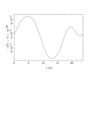
FIG. 1.: Variation during one day of the total squared signal from a NS distribution concentrated in the Galactic disk, according to Eqs. (A22) and (A23) with the parameters $\overline{\epsilon^{2}}=(10^{-8})^{2}$, $\overline{I^{2}}=(10^{38}{\rm\ kg\,m}^{2})^{2}$, $\overline{P^{-4}}=(5{\rm\ ms})^{-4}$, $R_{0}=3.8{\rm\ kpc}$ and $z=0.5{\rm\ kpc}$. The localization and orientation of the detector are those of VIRGO. $t=0$ corresponds to a zero local sidereal time.

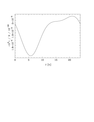
FIG. 2.: Variation during one day of the total squared signal from a NS distribution corresponding to a Galactic halo, according to Eqs. (A22) and (A24) with the parameters $\overline{\epsilon^{2}}=(10^{-8})^{2}$, $\overline{I^{2}}=(10^{38}{\rm\ kg\,m}^{2})^{2}$, $\overline{P^{-4}}=(5{\rm\ ms})^{-4}$, and $a_{0}=10{\rm\ kpc}$. The localization and orientation of the detector are those of VIRGO. $t=0$ corresponds to a zero local sidereal time.

TABLE I.: Gravitational radiation data for five selected pulsars. The GW amplitudes on Earth, $h_{0}$, are computed according to Eq. (1) by assuming that $I=10^{38}{\ \rm kg\,m}^{2}$ (a representative value for a $1.4\,M_{\odot}$ neutron star). $\epsilon_{\scriptscriptstyle-6}$ is the ellipticity in units of $10^{-6}$. The maximum ellipticity and maximum GW amplitudes are derived by attributing the totality of the observed pulsar spin-down rate to the emission of gravitation radiation.

pulsar	distance	GW		GW	maximum	maximum	ellipticity
name		frequencies		amplitude	ellipticity	GW amplitude	to get $h_{0}=10^{-26}$
	$r{\ \rm[kpc]}$	$f{\ \rm[Hz]}$	$2f{\ \rm[Hz]}$	$h_{0}$	$\epsilon_{\rm max}$	$h_{0,\rm max}$	$\epsilon_{\rm detect}$
Vela	0.5	11	22	$1.1\times 10^{-27}\,\epsilon_{\scriptscriptstyle-6}$	$1.8\times 10^{-3}$	$1.9\times 10^{-24}$	$9.1\times 10^{-6}$	$=5\times 10^{-3}\,\epsilon_{\rm max}$
Crab	2	30	60	$1.9\times 10^{-27}\,\epsilon_{\scriptscriptstyle-6}$	$7.5\times 10^{-4}$	$1.4\times 10^{-24}$	$5.3\times 10^{-6}$	$=7\times 10^{-3}\,\epsilon_{\rm max}$
Geminga	0.16a	4.2	8.4	$4.7\times 10^{-28}\,\epsilon_{\scriptscriptstyle-6}$	$2.3\times 10^{-3}$	$1.1\times 10^{-24}$	$2.1\times 10^{-5}$	$=9\times 10^{-3}\,\epsilon_{\rm max}$
B1957+20	1.5	621	1242	$1.1\times 10^{-24}\,\epsilon_{\scriptscriptstyle-6}$	$1.6\times 10^{-9}$	$1.7\times 10^{-27}$	$9.1\times 10^{-9}$	$>\epsilon_{\rm max}$
J0437-4715b	0.14	174	348	$9.1\times 10^{-25}\,\epsilon_{\scriptscriptstyle-6}$	$2.9\times 10^{-8}$	$2.6\times 10^{-26}$	$1.1\times 10^{-8}$	$=0.4\,\epsilon_{\rm max}$

TABLE II.: Fourier spectrum of the solar flux at the latitude of Pisa.

frequency	period	identification	spectral component
$\nu$ [Hz]	$\nu^{-1}$ [h]		(arbitary units)
3.1688089E-08	8766.000	1 year	0.6391195
6.3376177E-08	4383.000	6 months	1.4378662E-02
1.1510698E-05	24.13214	$\nu_{\rm sol}-2\nu_{\rm ty}$	4.0333651E-02
1.1542386E-05	24.06589	$\nu_{\rm sol}-\nu_{\rm ty}$	0.4005030
1.1574074E-05	24.00000	$\nu_{\rm sol}$ (solar day)	1.836788
1.1605762E-05	23.93447	$\nu_{\rm sol}+\nu_{\rm ty}$ (sidereal day)	0.4006524
1.1637450E-05	23.86930	$\nu_{\rm sol}+2\nu_{\rm ty}$	3.9582606E-02
2.3084773E-05	12.03294	$2\nu_{\rm sol}-2\nu_{\rm ty}$	5.2575748E-02
2.3116459E-05	12.01645	$2\nu_{\rm sol}-\nu_{\rm ty}$	1.2078404E-02
2.3148148E-05	12.00000	$2\nu_{\rm sol}$	0.7087801
2.3179837E-05	11.98359	$2\nu_{\rm sol}+\nu_{\rm ty}$	1.4178075E-02
2.3211524E-05	11.96724	$2\nu_{\rm sol}+2\nu_{\rm ty}$	5.2661020E-02

TABLE III.: Fourier spectrum of the total squared signal $\langle h^{2}(t)\rangle$ corresponding to a disk distribution of NS and depicted in Fig. 1.

frequency	cosine coef.	sine coef.
	(arbitary units)	(arbitary units)
0	7.895	0
$\nu_{\rm sid}$	0.923	0.593
$2\nu_{\rm sid}$	-0.738	-0.065
$3\nu_{\rm sid}$	-0.079	0.124
$4\nu_{\rm sid}$	0.005	0.087

REFERENCES

- [1] S. Bonazzola, J.-A. Marck, Annu. Rev. Nucl. Part. Sci. 45, 655 (1994)
- [2] J.-A. Marck, J.-P. Lasota (eds.), Relativistic Gravitation and Gravitational Radiation, Proc. of Les Houches School (26 September - 6 October 1995), Cambridge University Press, Cambridge, England, in press.
- [3] I. Ciufolini, F. Fidecaro (eds.), Proc. of the International Conference on Gravitational Waves: Sources and Detectors, Cascina (Pisa) (March 19-23, 1996). World Scientific, Singapore, in press.
- [4] J.R. Ipser, Astrophys. J. 166, 175 (1971)
- [5] M.A. Alpar, D. Pines, Nature 314, 334 (1985)
- [6] P. Haensel, in ref. [2] (preprint astro-ph/9605164)
- [7] D.V. Gal’tsov, V.P. Tsvetkov, A.N. Tsirulev, Zh. Eksp. Teor. Fiz. 86, 809 (1984); English translation in Sov. Phys. JETP 59, 472
- [8] S. Bonazzola, E. Gourgoulhon, Astron. Astrophys. 312, 675 (1996)
- [9] M. Zimmermann, E. Szedenits, Phys. Rev. D 20, 351 (1979)
- [10] R.V. Wagoner, Astrophys. J. 278, 345 (1984)
- [11] D. Lai, S.L. Shapiro, Astrophys. J. 442, 259 (1995)
- [12] J.R. Ipser, R.A. Managan, Astrophys. J. 282, 287 (1984)
- [13] S. Bonazzola, J. Frieben, E. Gourgoulhon, Astrophys. J. 460, 379 (1996)
- [14] F. Barone, L. Milano, I. Pinto, G. Russo, Astron. Astrophys. 203, 322 (1988)
- [15] W. Velloso, F. Barone, E. Calloni, L. Di Fiore, A. Grado, L. Milano, G. Russo, Gen. Rel. Grav., 28, 613 (1996)
- [16] E. Gourgoulhon, S. Bonazzola, in ref. [3] (preprint astro-ph/9605150)
- [17] J.H. Taylor, R.N. Manchester, A.G. Lyne, Astrophys. J. Suppl. 88, 529 (1993)
- [18] J.H. Taylor, R.N. Manchester, A.G. Lyne, F. Camilo, unpublished work (1995)
- [19] K.C.B. New, G. Chanmugam, W.W. Johnson, J.E. Tohline, Astrophys. J. 450, 757 (1995)
- [20] B.F. Schutz, in: The detection of gravitational waves, Blair D.G. (ed.). Cambridge University Press, Cambridge, England (1991)
- [21] K. Jotania, S.V. Dhurandhar, Bull. Astr. Soc. India 22, 303 (1994)
- [22] K. Jotania, S.R. Valluri, S.V. Dhurandhar, Astron. Astrophys. 306, 317 (1996)
- [23] T. Suzuki, in: First Edoardo Amaldi Conference on Gravitational Wave Experiments, eds. E. Coccia, G. Pizzella, F. Ronga, World Scientific, Singapore (1995)
- [24] S.V. Dhurandhar, D.G. Blair, M.E. Costa, Astron. Astrophys., 311, 1043 (1996)
- [25] E.E. Flanagan, Phys. Rev. D 48, 2389 (1993)
- [26] B. Allen, in ref. [2] (preprint gr-qc/9604033)
- [27] J.D. Kraus, Radio astronomy. McGraw-Hill, New York (1966)
- [28] S. Johnston et al., Nature 361, 613 (1993)
- [29] J.-Y. Vinet, private communication.
- [30] P.R. Saulson, Phys. Rev. D 42, 2437 (1990)
- [31] F. Bondu, J.-Y. Vinet, Phys. Lett. A 198, 74 (1995)
- [32] F.X. Timmes, S.E. Woosley, T.A. Weaver, Astrophys. J. 457, 834 (1996)
- [33] N.E. White, F. Nagase, A.N. Parmar, in: X-ray binaries, W.H.G Lewin, J. van Paradijs, E.P.J. van den Heuvel (eds.). Cambridge University Press, Cambridge, England (1995)
- [34] J. van Paradijs, in: The lives of the neutron stars, M.A. Alpar, Ü Kiziloglu, J. van Paradijs (eds.). Kluwer Academic Publishers, Dordrecht (1995)
- [35] F.M. Walter, S.J. Wolk, R. Neuhäuser, Nature 379, 233 (1996)
- [36] M. Salgado, S. Bonazzola, E. Gourgoulhon, P. Haensel, Astron. Astrophys. 291, 155 (1994)
- [37] D. Bhattacharya, in X-ray binaries, eds. W.H.G. Lewin, J. van Paradijs, E.P.J. van den Heuvel (eds.). Cambridge University Press, Cambridge, England (1995)
- [38] A.G. Lyne, in: The lives of the neutron stars, M.A. Alpar, Ü Kiziloglu, J. van Paradijs (eds.). Kluwer Academic Publishers, Dordrecht (1995)
- [39] S.J. Lilly, O. Le Fèvre, F. Hammer, D. Crampton, Astrophys. J. 460, L1 (1996)
- [40] P. Madau, H.C. Ferguson, M.E. Dickinson, M. Giavalisco, C.C. Steidel, A. Fruchter, submitted to Mon. Not. R. Astron. Soc. (preprint astro-ph/9607172)
- [41] V. Urpin, U. Geppert, Mon. Not. R. Astron. Soc. 275, 1117 (1995)
- [42] D. Bhattacharya, G. Srinivasan, in X-ray binaries, eds. W.H.G. Lewin, J. van Paradijs, E.P.J. van den Heuvel (eds.). Cambridge University Press, Cambridge, England (1995)
- [43] Giazotto A. et al., in First Edoardo Amaldi Conference on Gravitational Wave Experiments, eds. E. Coccia, G. Pizzella, F. Ronga, World Scientific, Singapore (1995).
- [44] A. Burrows, J. Hayes, Phys. Rev. Lett. 76, 352 (1996)
- [45] P.A. Caraveo, G.F. Bignami, R. Mignani, L.G. Taff, Astrophys. J. 461, L91 (1996)