Evolution in the X–ray Cluster Luminosity Function Revisited

Abstract

We present new X–ray data taken from the ROSAT PSPC pointing archive for 21 clusters in the Einstein Extended Medium Sensitivity Survey (EMSS). We have supplemented these data with new optical follow–up observations found in the literature and overall, 32 of the original 67 $z>0.14$ EMSS clusters now have new information. Using this revised sample, we find no systematic difference, as a function of X–ray flux, between our measured X–ray cluster fluxes and those in the original EMSS ($\simeq 30\%$ scatter). However, we do detect a marginal correlation between this observed difference in the flux and the redshift of the clusters, with the lower redshift systems having a larger scatter by nearly a factor of two. We have also determined the X–ray extent of these re–observed EMSS clusters and find 14 of them have significant extents compared to the ROSAT Point–Spread Function. Combining these data with extended clusters seen in the original EMSS sample, at least 40% of $z>0.14$ clusters now have an observed x–ray extent thus justifying their classification as X–ray clusters.

Using our improved EMSS sample, we have re–determined the EMSS X–ray Cluster Luminosity Function as a function of redshift. We have removed potential mis–classifications and included our new measurements of the clusters X–ray luminosities and redshifts. We find similar luminosity functions to those originally presented by Henry et al. (1992); albeit with two important differences. First, we show that the original low redshift EMSS luminosity function is insufficiently constrained. Secondly, the power law shape of our new determination of the high redshift EMSS luminosity function ($z=0.3\rightarrow 0.6$) has a shallower slope than that seen by Henry et al. . We have compared our new EMSS luminosity functions with those recently derived from nearby sample of X–ray clusters and find that the overall degree of observed luminosity function evolution is mild at best. This is a result of the shallower slope seen in our EMSS high redshift luminosity function and a more robust low redshift determination of the X–ray cluster luminosity function from the literature.

We have quantified the degree of evolution seen in the X–ray cluster luminosity using several statistical tests. The most restrictive analysis indicates that our low and high redshift EMSS luminosity functions are statistically different at the $95\%$ level. However, other tests indicate that these low and high redshift luminosity functions only differ by as little as $1\sigma$. These data are therefore, consistent with no evolution in the X–ray cluster luminosity function out to $z\simeq 0.5$.

To appear in Ap. J.

Nichol et al. Evolution in the X–ray Cluster Luminosity Function Revisited

1 Introduction

One of the most striking results in observational cosmology over the past five years has been the report of rapid evolution in the space density of X–ray clusters out to $z\sim 0.5$. The strongest evidence for such evolution has been presented by [Gioia et al. 1990a] & [Henry et al. 1992] (H92) using a sample of clusters serendipitously detected in Einstein IPC pointings (the Einstein Extended Medium Sensitivity Survey: EMSS). They report that the luminosity function of X–ray selected clusters steepens significantly as a function of redshift with the most distant cluster sample having nearly an order of magnitude less X–ray luminous clusters ($>10^{45}\,{\rm erg\,s^{-1}}$) than the present epoch.

In recent years, observations by the ROSAT X–ray satellite have focused on extending the redshift baseline of these evolutionary studies and overall, the results qualitatively agreed with the original findings of [Henry et al. 1992]. For example, all the specific deep PSPC pointings towards known optically rich, distant clusters of galaxies ($z>0.6$) have yet to discover a single X–ray bright cluster ([Nichol et al. 1994], [Castander et al. 1994] & [Bower et al. 1994]). These studies however, may be biased since most of their original targets were drawn from optically selected catalogues.

In the long term, such bias can be removed by compiling serendipitous samples of distant X–ray clusters from the large archive of ROSAT PSPC pointings in the same vein as the EMSS. Several groups have already begun this task and their combined effort should provide a powerful database for quantifying the degree of observed X–ray cluster evolution ([Castander et al. 1995], [Rosati et al. 1995], [Burke et al. 1995], [Scharf et al. 1997] & [Romer et al. 1997]). This work is still in its infancy, mainly because of the large amount of optical follow–up needed to verify the presence of a distant X–ray cluster and to exclude possible contaminants like stars and AGNs. Preliminary results from these ROSAT surveys either appear to be consistent with the EMSS sample (see [Castander et al. 1995]), or, advocating no evolution (see [Collins et al. 1997]).

The theoretical consequences of X–ray cluster luminosity evolution are significant, suggesting that the large–scale structure in the universe evolved hierarchically over a relatively short look–back time. However, the present results are inconsistent with simple scale–invariant hierarchical clustering models, since these actually predict an increase in X–ray bright clusters with increasing redshift ([Kaiser 1986]). Several authors have resolved this discrepancy but at the expense of breaking scale–invariance and allowing significant energy input into the gas at high redshift ([Kaiser 1991], [Evrard & Henry 1991], [Cavaliere et al. 1993]). Alternatively, the problem could be alleviated by steepening the slope of the initial density power spectrum on cluster scales, yet this would be inconsistent with popular Cold Dark Matter theories of structure formation ([Davis et al. 1985], [Henry et al. 1992]).

Considering the underlying theoretical importance of cluster evolution, we report here a re–examination of the EMSS cluster sample since this database is the most robust, well–understood catalogue of X–ray clusters out to $z\simeq 0.5$ presently available. The EMSS, as a whole, has received intense optical scrutiny over the past decade and many of its 835 X–ray sources now have a secure identification ([Gioia et al. 1990b], [Stocke et al. 1991]). In the next section, we describe new data available from the ROSAT pointing archive on nearly half of the $z>0.14$ EMSS clusters used by H92 in their evolutionary study. These new data therefore, provide an important check since many of these distant EMSS clusters were only $\simeq 5$ sigma detections in the Einstein data, i.e. there is a large uncertainty on their X–ray fluxes. The ROSAT re–observations of these clusters represent a significant improvement on this for three reasons: First, the clusters received, on average, longer exposure times; second, ROSAT has a much lower particle background thus improving its sensitivity to low surface brightness, extended objects; third, the satellite has greater on–axis angular resolution.

This new ROSAT dataset has allowed us to test two critical concerns about the EMSS cluster sample: i) the accuracy of the X–ray cluster fluxes and therefore, their luminosities; ii) the classification of the X–ray emission as a hot, intracluster medium. The latter point is very important with regards to identication since X–ray point sources such as stars and AGNs dominate the X–ray source counts. Therefore, only a small error in classifying these objects as clusters, and vice versa, will make a large difference to the final X–ray cluster subsample. Therefore, the most secure signature of cluster emission is X–ray extent. This re–examination of the EMSS is part of a large project aimed at searching the ROSAT data archives for serendipitous observations of distant X–ray clusters; Serendipitous High–redshift Archival ROSAT Cluster (SHARC) survey (see [Burke et al. 1995], [Ulmer et al. 1995]). Throughout this paper we assume $H_{o}=50\,{\rm km\,s^{-1}\,Mpc^{-1}}$ and $q_{o}=0.5$ to be consistent with previous work.

2 New Data and Analysis

We present, in Table 1, all the $z>0.14$ EMSS clusters, from Table 2 of H92, for which new data are available including re-observations by the ROSAT satellite and/or further optical identification work by Gioia & Luppino (1994; GL94) and others. Column 1 gives the EMSS name of the clusters followed by, in column 2, the ROSAT pointing identification number. Column 3 presents the measured redshift of the clusters which were taken from GL94 or Carlberg et al. (1996). Columns 4, 5 & 6 give the results of our X–ray source analysis and indicates whether we find the cluster X–ray emission extended or not (the numbering given in column 6 is the same as that in Figures 1 and 2). Column 7 gives the PSPC off–axis angle (in pixels) of the clusters and indicates cases where the cluster was the original requested target of ROSAT; $\simeq 85\%$ of our ROSAT EMSS cluster re–observations were again accidental. Column 8 is the averaged PSPC exposure time (vignetted corrected), while column 9 gives the net source counts (within the bandpass $0.4\rightarrow 2.0\,$keV). Many of the re–observed EMSS clusters are detected to significantly higher signal–to–noises in our data than that used by H92. Columns 10 & 11 are the measured source and background X–ray count rates and the final four columns are the X–ray fluxes and total luminosities computed from these observed count rates in both the ROSAT and Einstein bandpasses.

The PSPC pointing data used in this paper were obtained from the GSFC ROSAT data archive and reduced using a suite of programs we have developed as part of the SHARC survey. We refer the reader to our forthcoming paper, [Romer et al. 1997], that describes in detail our data reduction techniques. However, for completeness, we briefly highlight the main features of our analysis here. The raw X–ray data were initially reduced using the methodology outlined by [Snowden et al. 1994]. For each pointing, an individual exposure map was constructed from the satellite’s orbital information and divided into the binned X–ray photon data (15 arcsecond pixels). We concentrated on the “hard” ROSAT band, $0.4\rightarrow 2.0\,$keV, since this substantially reduces the background count rate. The exposure and vignetted corrected images were then analysed using our own source detection algorithm which is based on a mexican–hat wavelet transform. This particular wavelet is well–suited to analysing PSPC data since it is the second derivative of a Gaussian and therefore, this underlying function matches closely the (radially averaged) shape of the ROSAT Point Spread Function (PSF) which can be approximated by a Gaussian.

A crucial part of our re–analysis of the EMSS sample was to determine if the observed X–ray cluster emission was extended or not. For this reason, we present this particular stage of the analysis in greater detail. The extent of all sources in a pointing was determined directly from our wavelet data taking advantage of the fact that the width of the mexican hat filter, at it’s zero–crossing points, is equal to the width (between inflection points) of the original Gaussian it was constructed from. Therefore, we grew each source outwards from its initial centroid until we reached zero in wavelet–space. This source boundary, in wavelet–space, is then a measurement of the size of that source and is simply the product of the size of the mexican–hat (we define this as $\sigma_{w}$ which is the dispersion of the underlying Gaussian) and the size of the observed source, which in most cases will be the PSF. A final centroid analysis is then carried out on each candidate source, using only the pixels within this zero–crossing boundary, and their major and minor axes determined.

This procedure was independently carried out for three different mexican–hat sizes; $\sigma_{w}=$ 3, 6 and 9 pixels. The power of this approach is that the different size filters are sensitive to different regimes of the off-axis PSF. The smallest filter is best suited to the inner region of the PSPC field–of–view, while further off–axis, the larger filter sizes become more powerful as the PSF increases. For example, at large off-axis angles, the smallest filter tends to break–up sources because the surface brightness profiles of sources flattens due to increases in the PSF and reduction in the ROSAT telescope effective collecting area. The $\sigma_{w}=$ 6 and 9 pixel filters help to recover from this. Therefore, by changing the filter size in our analysis, we naturally accommodate for a changing PSF thus allowing us to probe further out into the ROSAT field–of–view.

Figures 1 and 2 shows the distribution of the major and minor axes, as a function of off-axis angle, for 1637 high signal–to–noise sources detected in the $\sigma_{w}=3$ wavelet maps of 407 deep ROSAT PSPC pointings. The size of the these sources is the convolution of the wavelet size with the intrinsic source size and therefore, they are larger expected. These pointings have been reduced as part of the SHARC survey which is presently investigating all extended sources seen in these data. The other $\sigma_{w}$ maps are very similar and are therefore, not shown. The only difference, as highlighted above, is the area over which the PSF locus is well–defined has been shifted to higher off-axis angles. Clearly visible in Figure 1 is the expected increase in the ROSAT PSF with off–axis angle above which we must determine if a source is extended or not. Also shown is a line which represents sources that are $>3\sigma$ extended and was empricially determined, as a function of off–axis angle, from these sources (see [Romer et al. 1997] for further information).

The off–axis angle and major and minor axes of all EMSS clusters detected in the 3 pixel wavelet map are presented in Table 1 (column 6) and are plotted in Figures 1 and 2. An EMSS cluster is designated as extended if its major and/or minor axis is above this $3\sigma$ line in any of the 3 wavelet maps, for example, MS0811.6+6301 was selected as extended based solely on the $\sigma_{w}=6$ wavelet information. A question mark in Table 1 signifies clusters that do not satisfy these criteria, but appear to lie away from the point–source locus in two or more of its wavelet representations.

The X–ray count rates of the EMSS clusters were measured interactively using the IRAF/PROS software package. This differs from the approach used in the SHARC survey and therefore, we describe it fully here. In the original EMSS, the cluster count rates were computed within a fixed angular aperture ($2.4\times 2.4$ arcmins) and were later corrected, via a cluster model, to the total X–ray flux. We, however, had the freedom to select a fixed metric aperture thus scaling it sppropriately with redshift and the PSF for each individual cluster (we convolved the angular size of the metric aperture with the expected size of the PSF). For aa assumed King profile with a core radius of $0.25{\rm Mpc}$ and $\beta=\frac{2}{3}$, we computed the angular size of an aperture for each cluster that would encompass 85% of the total cluster flux, irrespective of redshift and off–axis angle (the fluxes and luminosities given in Table 1 are corrected for the 15% of light expected outside the aperture). Furthermore, the interactive approach allowed us examine the environment of each cluster and exclude any nearby sources (both in the background and source apertures). Wherever possible, the background was estimated from an annulus around the source aperture having a similar number of pixels as the source aperture. If this was not possible, a nearby area devoid of sources was used, ensuring that it was at the same off-axis distance as the source so the vignetting corrections would be comparable.

These measured count rates were finally converted to fluxes (${\rm erg\,cm^{-2}\,s^{-1}}$) by integrating a 6keV Raymond–Smith (RS) spectrum through the ROSAT response function and accounting for absorption using HI column densities interpolated from Stark et al. (1992) and the model by Morrison & McCammon (1983). This therefore, gave us the X–ray cluster flux in the ROSAT bandpass outside our own Galaxy. We then converted the ROSAT fluxes to that expected in the Einstein bandpass again using a 6keV RS spectrum. We chose this model cluster spectrum to be fully consistent with the H92 analysis. The cluster luminosities (including k–corrections) for both the ROSAT and EMSS bandpasses are given in columns 14 & 15 of Table 1 respectively.

Ideally, we would like to convert our ROSAT count rates to Einstein fluxes using the individual spectra of these EMSS clusters. However, for a vast majority of the EMSS such data does not exist. Therefore, to quantify this potential systematic effect, we re–computed the expected Einstein fluxes of all our ROSAT EMSS detections using the Luminosity–Temperature relationship of [Wang & Stocke 1993] and iterated it until we gained a stable solution (within 0.1% between iterations). This usually took $<4$ passes and always changed the final iterated cluster luminosity by less than 6%. For example, MS0015.9+1609 shifted from ${\rm L_{x}(44)}=22.78\,{\rm erg\,s^{-1}}$ – which is given in Table 1 – to ${\rm L_{x}(44)}=23.72\,{\rm erg\,s^{-1}}$ for an iterated temperature of 11.35keV. Our count rate to flux conversion was also relatively insensitive to variations in the RS metal abundance and varied by less than 10% over a reasonable range of metallicities.

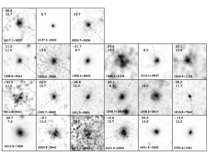
Figure 3: A greyscale plot of the count rates of the 21 EMSS cluster with new ROSAT data given in Table 1. North is upwards with East to the left. The solid line represents the measured position angle of the cluster and is only computed for clusters with ${\rm minor/major}>0.8$, thus avoiding circular clusters. The numerical value – in degrees – of the position angle is the top number shown in the top–left hand corner of the window. The dashed line is the direction towards the center of the PSPC and helps the reader determine if the asymmetrical PSPC PSF has influenced the determination of the position angle. In some cases, this looks likely. The dashed line is not plotted if the cluster was nearly on-axis. The count rate data are scaled linearly between zero and the maximum observed count rate (these maps have been vignetted and exposure corrected). The contribution of the PSF has not been removed and these images have also been lightly smoothed with a Gaussian of width one pixel to reduce the binning noise. The size of the plotting window is given as the bottom number in the top left–hand corner and is equal to the aperture used in the flux determination. Other sources near the cluster were removed prior to any flux determination i.e. MS1208.7+3928.

In Figures 3 and 4, we present all available ROSAT data on the distant $z>0.14$ EMSS clusters discussed in this paper. The size of the individual plotting windows in Figure 3 is equal to the diameter of the aperture used to compute the cluster count rates. Also shown is the measured position angle of the observed x–ray emission and the radial direction towards the center of the PSPC. In Figure 4, we present the ROSAT radial X–ray surface brightness profiles for the clusters as well as the appropriate off-axis ROSAT PSF. For the PSPC data, this was computed from the point–source locii seen in Figures 1 and 2 (not the $3\sigma$ line). For the HRI data, we used the model of David et al. (1993) for the PSF. These plots clearly show that many of the re–observed EMSS clusters are high signal–to–noise X–ray detections and are extended.

Table 2: Maximum likelihood Parameterisation of XCLFs derived from the original EMSS Data Sample

Redshift shell	Number	$\alpha$	$K(10^{7}Mpc^{-3}L_{44}^{\alpha-1})$
0.14 - 0.2	21	$2.24\pm 0.32$ ($2.19\pm 0.21$)	$7.5\pm 1.9$ ($5.85\pm 0.25$)
0.2 - 0.3	23	$2.72\pm 0.29$ ($2.67\pm 0.26$)	$7.6\pm 1.9$ ($6.82\pm 0.51$)
0.3 - 0.6	23	$3.37\pm 0.31$ ($3.27\pm 0.29$)	$14.8\pm 5.2$ ($12.33\pm 3.87$)

3 Comparison of Cluster X–ray Flux Measurements

One of the motivations of our work was to check the robustness of the EMSS flux measurements. In H92, the total flux was computed, using a King model, from the detected flux within a fixed angular aperture. In contrast, we attempt to measure the total flux directly using a fixed metric aperture. For the 21 ROSAT–EMSS clusters, Figure 5 presents the difference between our ROSAT mesurement of the total flux of the EMSS clusters in the Einstein bandpass (column 13 in Table 1) and that given by H92, versus our total ROSAT–EMSS flux. The error bars plotted in Figure 5 were derived from the propagation of the errors published on the net counts by H92 and in Table 1 of this paper (column 9). Using a $\chi^{2}$ test, we have compared the data in Figure 5 with the expected relationship i.e. the zero line in Figure 5. For all the data points, we find $\chi^{2}=57$ for 20 degrees of freedom (d.o.f) which is highly improbable. However, much of this disagreement is due to the two points at the highest total flux (MS0451.5+0250 and MS0735.6+7421). Therefore, if we constrain our analysis to ${\rm F_{x}<2\times 10^{-12}\,erg\,s^{-1}\,cm^{2}}$ and ${\rm F_{x}<10^{-12}\,erg\,s^{-1}\,cm^{2}}$, we find $\chi^{2}=33$ (18 d.o.f) and $\chi^{2}=12$ (12 d.o.f) respectively. These indicate that the observed scatter (28%) at lower flux levels is consistent with the observed errors on the two datasets (ours and H92).

Figure 1: The major and minor axes for 1637 high signal–to–noise sources detected in 407 deep ROSAT PSPC pointings versus their off-axis angle (the x–axis the convolution of the source size with the wavelet filter size). The change in the PSPC PSF with off-axis angle is visible and was defined empiricially (the dotted lines represent $>3\sigma$ extended sources). The star symbols are $z>0.3$ EMSS clusters and have the same numbering as given in column 4 of Table 1. The unfilled circles are the 2 EMSS clusters that only have lower limits measured for their extents. These sources were found in the $3$ pixel wavelet map.

Figure 2: The same as Figure 1 but showing the $z<0.3$ EMSS clusters (solid symbols). Again, the numbers coincide with those given in column 4 of Table 1.

A more interesting plot to make is to plot the flux differences in Figure 5 as a function of redshift. This is shown in Figure 6. In this case, there does appear to be a noticeable decrease in the flux differences with increased redshift. This is quantified by splitting the sample at $z=0.3$, with the lower redshift clusters having a mean absolute difference of 39%, while for the higher redshift data, the mean absolute difference is only 19%. The standard error on both these means is $\sim 30\%$, since both were determined using $\simeq 10$ clusters. Therefore, this observed drop in the mean absolute flux difference is marginally significant. Such a decrease with redshift is consistent with the H92 methodology since at higher redshifts there would be a greater amount of the clusters’ total flux within the fixed angular aperture compared to lower redshifts, thus the required correction would be smaller.

4 Measurement of Extended Cluster X–ray Emission

It is imperative that the classification of all EMSS clusters should be made as secure as possible. This is straightforward using the measured extent of the observed X–ray emission from the cluster. Figures 1 and 2 present the observed extent of our ROSAT–EMSS clusters against that expected for X–ray point–sources (as a function of off-axis angle). Overall, 14 of the 21 clusters with new ROSAT data are flagged extended in Table 1 (column 4). For 3 of these extended sources, H92 also detected an extent in the Einstein data (these clusters are highlighted in Table 1). By combining our extent results with H92, a total of 25 $z>0.14$ EMSS clusters now have sufficient X–ray information to measure a significant X–ray extent ($40\%$ of the whole EMSS sample). Constraining ourselves to $z>0.3$, this figure drops to $30\%$. For these extended clusters, therefore, we are most probably seeing X–ray emission from a hot, intracluster gas which undoubably strengthens their classification as X–ray clusters.

Next we discuss the clusters marked as non–extended, or uncertain, in our database. Some of these are the result of low signal–to–noise, low intrinsic X–ray luminosity and/or uncertainties in the PSF at large off–axis angles. For example, MS0418.3–3844 is very close to the ROSAT rib structure resulting in an unrealistic major and minor axis in all 3 wavelet maps and therefore, we only present a lower limit to the cluster size in Table 1. The same problem occurred for MS811.6+6301 in the $\sigma_{w}=3$ wavelet map, but it was observed to be extended in the larger wavelet maps.

For EMSS clusters MS1209.0+3917, MS1219.9+7542, MS1512.4+3647 and MS2137.3-2353, there exists significant archival ROSAT HRI data which can help classify these systems. In the PSPC data, they all lie on – or near – the observed point source locus in all three wavelet maps (see Figures 1 and 2). They also appear unextended in Figure 4 Considering the length of exposure time gained in these PSPC data, we suggest that these clusters either have compact cores, or, that they are mis-identifications. For MS1209.0+3917 and MS1219.9+7542, the HRI indicates that these X–ray sources are point–like with little evidence for any X–ray extent. The optical CCD image of MS1209.0+3917 by GL94, and their own suspicions, supports the idea that this cluster is a mis-identification. For MS1219.9+7542, this system is a poor group with a dominant galaxy showing moderate [OII] emission in its’ optical spectrum (GL94 and Stocke et al. 1991). The X–ray and optical data combined, appears to indicate that the x-ray emission for these two EMSS clusters may be due to an AGN and not a hot, intracluster medium. We therefore, remove these clusters in any further analysis of the EMSS sample.

For MS2137.3-2353 and MS1512.5+3647, the HRI data indicates that the X–ray emission from these systems is extended compared to the PSF. We fitted a King model to the HRI data and measured core radii of $17\pm 8$ ($\beta=0.77\pm 0.28$) and $16\pm 10$ ($\beta=0.63\pm 0.23$) arcseconds for MS2137.3-2353 and MS1512.5+3647 respectively. Clearly, both clusters could not have been expected to be resolved by the PSPC instrument since even on-axis, the PSPC PSF has a $\simeq 20$ arcseconds FWHM (illustrated in Figure 4). For both systems, the angular extent of the X–ray emission represents a metric core radius of less than $100$ kpc; significantly smaller than the rest of the EMSS sample. For MS2137.3-2353, the lensing work of Mellier et al. (1993) agrees with this metric core radius, while the optical appearance of this system is dominated by a single, large cD–like galaxy with a similar metric size as the observed X–ray emission (GL94). For MS1512.5+3647, Stocke et al. (1991) has classified this system as a “cooling–flow galaxy” which is defined to be a galaxy with similar optical characteristics as the dominant galaxy in a cooling flow clusters but which is no associated with a rich, optical cluster of galaxies (see the CCD image in GL94). Carlberg et al. 1996 has extensive redshift information on this EMSS cluster and measure a velocity dispersion of $\sigma_{v}=690\,{\rm km\,s^{-1}}$. However, this system appears to have substantial redshift contamination (as seen in Figure 1 of their paper) and may indicate that MS1512.5+3647 is a projection effect. More data are required on these two systems to unambiguously classify them. We do not remove MS2137.3-2353 and MS1512.5+3647 in our later analysis, but note that our results were quite insensitive to their inclusion, or, removal.

No high quality ROSAT HRI data exists for the remaining 2 clusters marked as non–extended, or uncertain, in Table 1 (MS1208.7+3928 & MS1617.1+3237). For these two, we therefore performed Monte Carlo simulations to assess whether we had the required signal–to–noise to observe an extent or not (these simulations are presently being developed as part of the SHARC survey to help characterise the selection function of that survey and will be presented in detail in a forthcoming paper). Briefly, the simulations used here involved adding false clusters to the relevent ROSAT PSPC pointings (Table 1) using an underlying King profile of core radius $0.25$ Mpc and $\beta=\frac{2}{3}$. These false clusters were given the same signal–to–noise as the real real detections and were positioned at the same off–axis angle (usually opposite the real cluster in the PSPC field–of–view). For each cluster, 10 iterations were constructed and passed through our source detection software. This allowed us to determine the frequency with which these false sources were flagged as extented. Using these simulations as a guideline, it would appear that MS1208.7+3928 is more compact than expected since it was always detected as extended in the simulations. MS1617.1+3237, however, remains uncertain since the simulations indicated that we do not have high enough signal–to–noise to unambigously detect an extent given this nominal profile (it was flagged as extended only $\simeq 70\%$ of the time).

5 The X–ray Cluster Luminosity Function

5.1 A Re–Determination of the H92 Result

As mentioned earlier, the most striking result to come out of the EMSS cluster sample is evidence for rapid negative evolution in the X–ray Cluster Luminosity Function (XCLF; H92). Considering the amount of new information gained on the EMSS sample of clusters over the past few years, we have revisited the H92 result here. Our motivation for this are two–fold: First, to determine if actual changes in specific clusters make a significant systematic difference to the observed XCLF; secondly, to assess the robustness of the result to small, yet significant, changes in the overall cluster population. For instance, if the XCLF was radically altered, in any sense, by changes to a few clusters, it would indicate that the sample was not stable and remove much of its predictive power. In conjunction, we have re-assessed the statistical significance of X–ray evolution originally reported by H92.

Figure 4: The radially–averaged profiles for 21 EMSS clusters with new ROSAT PSPC data (given in Table 1) and 4 EMSS clusters with available HRI data. The x–axis is in arcseconds from the intensity–weighted centroids of the clusters, while the y–axis is the observed X–ray surface brightness (${\rm counts\,s^{-1}\,arcsec^{-2}}$). The binsize used for the PSPC and HRI data was 20 and 6 arcseconds respectively. The dashed lines show the expected size of the PSF at that given off-axis angle (as given in Table 1). The PSPC PSF was empirically determined from the data given in Figures 1 and 2 (we use the observed point–source locus not the $>3\sigma$ line shown). The HRI PSF was taken from David et al. 1993

We initially re–computed the XCLF using the same $1/V_{a}$ test as employed by H92 ([Avni & Bahcall 1980]). This involved computing the maximum observable volume ($V_{a}$) for each cluster,

$$V_{a}=\sum_{i=1}^{N}\Omega_{i}\Delta V(z_{max},z_{min}),$$ (1)

where $\Omega_{i}$ is the area of the EMSS survey to a given sensitivity limit (see Table 3 in H92), $N$ is the total number of different sensitivity limits (19 in total from Table 3 in H92) and $z_{min}$ is the lower redshift limit for a given redshift shell. For $z_{max}$, the smaller of either the maximum detectable redshift for a given cluster, or, the high redshift limit in a given redshift shell was used. The maximum detectable redshift was computed in the same fashion as in H92 (Eqn. 2 in their paper) using the sensitivity limits in Table 3 of H92 and either our new ROSAT determination of the cluster luminosity (using the same csomology and k–corrections) or that given in Table 2 of H92 (for clusters with no new ROSAT information).

These individual cluster volumes were then converted into a XCLF by binning them as a function of luminosity according to

$$n(L)=\sum_{j=1}^{n}\frac{1}{V_{a,j}\,\Delta L},$$ (2)

where $n$ is the number of clusters in the luminosity bin $\Delta L$ wide. Again, we use new ROSAT measurements of the clusters X–ray luminosities where appropriate. Before we discuss our new determinations of the EMSS XCLFs, we note that we reproduced the binned H92 XCLFs as shown in Figure 2 of their paper using only the data given in Table 2 of H92. The re–determinations of the H92 XCLFs are shown in Figure 7 for comparison and serve as a good check of our methodology.

Meanwhile, Figure 8 shows our new determinations of the EMSS XCLFs in the same three redshift shells as used by H92; z=0.14 to 0.2, 0.2 to 0.3 and 0.3 to 0.6. We have used, where appropriate, the new data presented in Table 1 of this paper, which includes removing clusters that we have flagged as either unextended or uncertain (see the discussion above and Table 1 where we have marked removed clusters with a $\star$). For clusters with no new information associated with them, we simply used the original fluxes and luminosities quoted in H92. Poisson error bars are shown and were obtained from the confidence limits tabulated by [Gehrels 1986].

Table 3: Maximum likelihood Parameterisation of XCLFs derived from our New EMSS Data Sample

Redshift shell	Number	$\alpha$	$K(10^{7}Mpc^{-3}L_{44}^{\alpha-1})$
0.14 - 0.2	19	$2.44\pm 0.34$ ($2.19\pm 0.21$)	$7.9\pm 1.8$ ($5.85\pm 0.25$)
0.2 - 0.3	21	$2.66\pm 0.30$ ($2.67\pm 0.26$)	$6.5\pm 1.7$ ($6.82\pm 0.51$)
0.3 - 0.6	21	$3.03\pm 0.30$ ($3.27\pm 0.29$)	$7.9\pm 3.0$ ($12.33\pm 3.87$)
0.14 - 0.3	40	$2.62\pm 0.22$	$7.2\pm 1.3$
With Luminosity Errors
0.14 - 0.2	19	$2.60\pm 0.37$	$8.7\pm 2.0$
0.2 - 0.3	21	$2.73\pm 0.31$	$7.0\pm 1.8$
0.3 - 0.6	21	$3.08\pm 0.32$	$8.5\pm 3.4$

Clearly, the three new XCLFs presented in Figure 8 are similar to those shown in H92 and Figure 7. This indicates that the EMSS sample is internally robust, since 50% of the clusters used in our new EMSS XCLFs have either a changed classification (cluster or not), a new flux measurement (different by up to 60%), and/or a new redshift. Certain clusters have changed substantially in luminosity, populating different bins in our XCLF than they did in the H92 result. This is certainly true in the highest redshift shell where the 2 clusters MS0015.9+1609 and MS0451.6-0305 have been elevated in total luminosity to occupy a previously unoccupied bin centered at $2.5\times 10^{45}\,{\rm erg\,s^{-1}}$. We note here that other re–determinations of the ROSAT flux for these two clusters are in good agreement with ours (Hughes, private communication, Neumann & Böhinger 1996, Donahue & Stocke 1995).

Figure 5: The percentile difference between our estimate of the EMSS total flux (derived from our ROSAT data) and the total EMSS flux quoted by H92, as a function of our estimate of the EMSS total flux. The errors plotted were derived from the combinations of the errors on the net counts given in H92 and our errors in Table 1.

Figure 6: The same as Figure 4, but plotted as a function of EMSS cluster redshift.

However, these binned XCLFs do not allow us to judge the statistical significance of our work and therefore, we parameterised our luminosity functions using a power-law luminosity function of the form, $n(L_{44})=K\,L_{44}^{-\alpha}$, where $L_{44}$ is the clusters luminosity in units of $10^{44}\,{\rm erg\,s^{-1}}$ (H92). For every cluster in a particular redshift shell, we compute the probability that we would see this cluster, at that luminosity, given the sensitivity limits of the EMSS (in H92 Table 3) and the model. This probability ($P$) can be expressed in full as,

$$P(L_{i})=\frac{1}{N}\int_{-\infty}^{\infty}V(L)\,L^{-\alpha}\,\delta(L_{i}-L)\,dL,$$ (3)

where $L_{i}$ is the observed luminosity of a cluster (taken from Table 1 of this paper or Table 2 from H92), $V(L)$ is the available volume within which that cluster could have been seen and $\delta(L_{i}-L)$ is a delta function which is unity at $L_{i}$ and zero for all other values of $L$. This, therefore, assumes no error on the observed luminosities (see below) and Eqn. 3 can be reduced to

$$P(L_{i})=\frac{1}{N}V_{a}\,L_{i}^{-\alpha}\,\Delta L,$$ (4)

where $V_{a}$ is given in Eqn. 1 (the available search volume of the cluster) and $\Delta L$ is chosen to be vanishingly small so only a $L_{i}$ cluster can fall within this interval (see Cash 1979 for full details). In Eqn. 3 and 4, $N$ is the normalisation such that

$$N=\int_{L_{min}}^{\infty}\,V(L)\,L^{-\alpha}\,dL$$ (5)

intergrated over the entire same range of luminosities. The likelihood of a given model is therefore,

$${\cal L}(\alpha)=\prod_{i=1}^{n_{obj}}\,P(L_{i}|\alpha)$$ (6)

using Equations 3,4 and 5.

Since our ML method is slightly different from the approach implemented by H92, we ensured that our ML fits to the original H92 data were compatible with those published in their paper. In other words, we attempted to fully reproduce the H92 result using only the data in Table 2 of their paper. We summarise these results in Table 2 and the fits are shown in Figure 7. Overall, we obtained excellent agreement with the H92 results with only one significant discrepancy; we see a $50\%$ large error on the low redshift XCLF than H92 (In Tables 2 and 3, we present in parentheses the slopes, and errors, on all 3 EMSS XCLFs as published in H92). The source of this discrepancy remains unclear but may be the result of us have a different likelihood distribution, for this low redshift shell, than H92 and Gioia et al. (1990a). This would effect our error analysis because we integrated the observed likelihood distribution directly, while H92 and Gioia et al. (1990a) used an analytical approach which assumes the likelihood distribution is a Gaussian (Gioia, private communication). We performed this latter approach on our data and did find a smaller error on the slope of the low redshift EMSS XCLF compared to that presented in Table 2. However, it was not large enough to fully explain this discrepancy between us and H92.

Figure 7: Binned X–ray Cluster Luminosity Functions in three redshift shells. These were computed by us using only the original data in H92 (we have used different bin centers to those used by H92). The solid line represents our best ML fit while the dotted line is the best ML fit from H92.

Figure 8: Binned X–ray Cluster Luminosity Functions in three redshift shells. In this case, we have used the improvements detailed in Table 1 of this paper in conjunction with data from the original H92 data. The solid line represents our best ML fit as seen in Table 2. The square symbol in the bottom plot represents the volume density of very high redshift EMSS clusters discussed in the text.

Table 3 summaries the ML parameterisations of our new EMSS XCLFs and includes (in parentheses) the original H92 results for comparison. The normalisation of the power–law XCLF (K) was computed by requiring Eqn. 5 to give the observed number of clusters. Our ML parametric representations are in reasonable agreement with those published by H92. This should not be too surprising given the visual similarity in the binned XCLFs. The largest discrepancy is in the slope of the highest redshift XCLF, where we find a shallower slope than H92 by $\simeq 1\sigma$. This change is almost exclusively due to the increased dynamic range in luminosity we are probing since we have a new highest luminosity bin compared to H92. We also find that our determination of the low redshift XCLF has a steeper slope compared to the original H92 result (we were able to re–produce the H92 slope when we used only their data). This is somewhat surprising since we have only changed 4 clusters in this redshift shell (2 changed in luminosity and 2 clusters were removed; see Table 1). We have investigated this discrepancy by re–computing the low redshift XCLF removing each of these 4 clusters one at a time. The most significant effect is noticed when MS2318.7-2328 is removed because of a lower redshift measurement by Romer (1994). This cluster is the highest luminosity cluster in the original H92 determination of the low redshift XCLF and therefore, it is understandable that its’ removal has the largest effect on our XCLF re–determination (also it explains why we see a steeper slope since we have removed the highest luminosity cluster in that shell). Overall, this low redshift shell is poorly determined since it is very sensitive to small changes in the dataset.

To quantify the statistical significance of our ML fits, we present in Tables 2 and 3 the computed errors on our ML parameters. These were computed by re–normalising the observed likelihood distributions (by integrating over the whole distribution and dividing it by the total) for the three redshift shells and determining the interval that enclosed 68% of the values. Figure 9 presents our observed likelihood distributions for the three redshift shells and can be approximated by a Gaussian. This figure is extremely enlightening, since it shows that the slope ($\alpha$) of the low redshift parametric XCLF is insufficiently constrained since it has a wide likelihood distribution. Overall, the high redshift XCLF parameterisation is only mildly inconsistent with the low redshift data. The probability of not getting the high redshift slope – from the low redshift data – is only 93%. This is caused by a combination of the low dynamic range – in luminosity – that the low redshift data extends over and the changes in the XCLF slopes mentioned above. Moreover, the difference in slope between the low and middle redshift XCLFs is clearly insignificant with the probability of obtaining the middle redshift shell maximum likelihood slope – from the low redshift data – being 51%.

Since the error on the XCLFs is crucial to any measurement of XCLF evolution, we tested our ML error analysis by performed Monte Carlo simulations ($>2000$ iterations per XCLF). This involved generating fake cluster databases – with the same total number of clusters as the real data – drawn at random from the parameterised H92 XCLFs. For all three redshift shells, the mean of the subsequent distribution of fitted XCLF slopes measured for these fake cluster catalogues was identical to the original input values. Moreover, the distributions were Gaussian–like and had dispersions very similar to those presented in Tables 2 and 3. Therefore, our error estimates on the real XCLFs given in Tables 2 and 3 are consistent with the scatter expected for these number of clusters (in each redshift shell).

Figure 9: The likelihood distributions for the three different redshift EMSS X–ray Cluster Luminosity Functions. The dashed line is the combined luminosity function ($z=0.14$ to 0.3) discussed in the text. The solid points –with errors– represent the maximum likelihood slopes as tabulated in Table 2.

Figure 10: Comparison of the low redshift XCLF (solid line) with the high redshift XCLF (dotted line) and the XCLF of Ebeling et al. (1995, 1996) computed from the RASS (dashed line). The latter has been shifted to the same energy bandpass. The solid symbols ($\bullet$) are binned high redshift luminosity function, while the open circles ($\circ$) are the low redshift case. The solid square is the volume density of very high redshift ($z>0.6$) clusters and the arrow ($\uparrow$) marks the lower limit of Nichol et al. (1994) in this redshift range.

Figure 11: $V/V_{max}$ versus $L_{x}$ for the EMSS sample. The left–hand panel is for the combined low (0.14 to 0.3) redshift shell ($\bullet$) against the high redshift EMSS shell (open symbols). The right–hand panel is for the original low (0.14 to 0.2) redshift shell ($\star$) against the same high redshift shell data.

5.2 Further Tests of XCLF Evolution

In this section we move beyond the analysis used by H92 to incorporate different statistical tests and independent XCLF results published over the last few years. We also investigated splitting the sample into different redshift shells.

Our analysis has highlighted that the low redshift EMSS XCLF is insufficiently constrained. Recently, however, Ebeling et al. (1995, 1996) has published a new low redshift XCLF using the ROSAT All–Sky Survey (RASS) Brightest Cluster Sample comprising of 173 $z<0.3$ X–ray clusters. From their analysis, they found that the data was consistent with no XCLF evolution out to $z=0.3$. This can be seen in Figure 10, where we compare this new RASS XCLF with our re–determiations of the EMSS XCLFs. We have now combined the lower two redshift EMSS shells (i.e. $z=0.14$ to 0.3) since our analysis indicates that there is little statistical difference between the two. Furthermore, it helps in our search for evidence for XCLF evolution because it increases the dynamic range – in cluster luminosities – studied thus providing a greater constraint on the fitted ML parameters (see Figure 9 and Table 3).

Clearly, there is excellent agreement between the RASS XCLF and our combined lower redshift EMSS XCLF. This is very impressive since the two samples cover different redshift regimes i.e. the RASS sample only has $20\%$ ($8\%$) of its clusters at $z>0.14$ ($z>0.2$) – the lower limit of the EMSS data – and all having $L_{x}>5\times 10^{44}\,{\rm erg\,s^{-1}}$). The fact that these two XCLFs, from different surveys over different redshift ranges, agree so well justifies our original motivation for combining the two lower EMSS samples. Clearly, the emphasis should now be on determining the degree of evolution above $z=0.3$. We say this irrespective of our own work, since Ebeling et al. (1995, 1996) sees no evidence for evolution at redshifts lower than this using a much larger sample of clusters. We have therefore, compared this new combined lower redshift EMSS XCLF with that derived at high redshift. Although the fitted ML slopes of these two EMSS XCLFs are different ($z=0.14$ to 0.3 compared to $z=0.3$ to 0.6), a close inspection of Figure 9 and Table 3 highlights that this discrepancy is only mildly significant.

To quantify this significance, we have implemented a 2D Kolmogorov–Smirnov (KS) test, in the $L_{x}$–$V/V_{max}$ plane, comparing the two redshift shells, 0.14 to 0.3 and 0.3 to 0.6, from our improved EMSS sample. The $V/V_{max}$ was calculated using the approach outlines in Avni & Bahcall (1980) using a uniform density distribution. This statistical analysis removes the need for any binning, or fitting, of the data and directly test the hypothesis that these two distributions were drawn from the same underlying parent distribution. Therefore, for this application, it is a very powerful method. Figure 11 shows the data displayed in the $L_{x}$–$V/V_{max}$ plane for the two redshift shells mentioned above. A KS test of these two gives a probability of 15% that they were drawn from the same underlying distribution. This drops only slightly to 11% if we limit ourselves to comparing the $z=0.14$ to 0.2 shell to the high redshift shell. In these KS tests, we have constrained the data to $L_{x}(0.3-3.5)>10^{44}\,{\rm erg\,s^{-1}}$ since below this limit the high redshift shell starts to become seriously incomplete (the EMSS does not have the sensitivity to probe such clusters at these high redshifts). If we compare all the data without a luminosity cut, the above KS probabilities – that the two distributions are the same – are 9% and 5% respectively.

For comparison, we also computed the mean $V/V_{max}$ in the high redshift shell (over the same range of $L_{x}$) for both our improved EMSS sample and the original H92 sample. We found $0.44\pm 0.08$ for our data and $0.36\pm 0.06$ for H92 (the standard error on the mean is quoted). This again indicates that the evidence for evolution in the high redshift shell has decreased since our measured mean $V/V_{max}$ is now consistent with the expected value (0.5; [Avni & Bahcall 1980]).

Most statistical analyses of XCLFs do not include observed luminosity errors. As can be seen in Figures 5 and 6, this can be a large effect and a function of redshift. For completeness therefore, we re–computed our ML parameterisations of the XCLFs but replacing the delta function in Eqn. 3 by a Gaussian whose width is equal to the observed luminosity error (using either the error on the flux given in Table 2 of H92 or our error on the ROSAT flux in Table 1 of this paper). This is computationally intensive since for each cluster the probability of it being observed is now an integral over a range of possible luminosities (because of the error in the luminosity). The search volume for each possible luminosity is re–computed (Eqn. 1) since $z_{max}$ changes with luminosity.

In Table 3, we present these new ML parameterisation of the low, middle and high redshift EMSS XCLFs. As can be seen, their are two effects in adding such errors. First, all the slopes have steepened with respect to their previous determinations (with no errors). Second, the degree to which they have steepened is different for each redshift shell, with the lower redshift shells changing the most. Therefore, the statistical significance of any steepening with redshift of these slopes is now lessened; the low and high redshift shells are only inconsistent at the $1\sigma$ level.

Finally, we turn our attention to the form of the very high redshift XCLF i.e. $z=0.6$ to $0.9$. In the past few years, several groups have used the ROSAT satellite to extend the study of XCLF evolution into this redshift regime ([Nichol et al. 1994], [Castander et al. 1994]). Moreover, further optical follow–up by GL94 has revealed two new EMSS clusters that have $z>0.6$ (see also Luppino & Gioia 1995). Although the data are still very limited, we have plotted the volume density of these two very high redshift EMSS clusters as a single point in Figure 10. Also plotted is the lower limit for lower luminosity clusters in this redshift shell as derived by [Nichol et al. 1994]. In both case, these data are consistent with the lower redshift EMSS XCLFs.

Using the EMSS sensitivity limits given by H92, we have computed that the lowest detectable cluster luminosity in this very high redshift shell is $4.1\times 10^{44}\,{\rm ergs\,s^{-1}}$. Given the low redshift XCLF parameterisation (redshift 0.14 to 0.3; Table 3), we estimate that the EMSS should have detected a total of 10 clusters brighter than this limit at these very high redshifts (we would expect three of these clusters to have $L_{x}>10^{45}$). This discrepancy is either evidence for evolution in the bright end of the XCLF at these high redshifts, or, a reflection of the EMSS classification procedure (the highest redshift clusters are the hardest to find and measure).

6 Conclusions

We present in this paper a thorough re-examination of the EMSS cluster sample using new data from the ROSAT PSPC pointing archive. Furthermore, we include the latest information on the optical follow–up of this sample of clusters. In total, 32 of the original 67 $z>0.14$ EMSS clusters used by H92 to study X–ray cluster evolution have new information associated with them, of which, 21 have new X–ray data obtained from the ROSAT archive. For these clusters, we find no systematic difference, as a function of X–ray flux, between the original EMSS flux estimates and our ROSAT re–determinations ($28\%$ scatter). Our analysis did however, indicate that this scatter may be correlated with cluster redshift with the high redshift clusters having a lower scatter by a factor of two. This is consistent with the expected trend given that the original EMSS fluxes were computed within a fixed angular aperture.

We determined the extent for 21 of the ROSAT re-observed clusters, of which, 14 were clearly extended compared to the ROSAT point–spread function. Combining this with results from H92, 40% of the $z>0.14$ EMSS clusters are extended in the X–rays thus securing their classifications as X–ray clusters. For the other 7 clusters, only 2 were definitely classed as point–like X–ray sources and the optical follow–up work of these clusters supports the idea that these maybe mis–classifications. The remaining 5 clusters are uncertain, either due to a lack of signal–to–noise to make a conclusive statement on their extent, or, they simply resist easy categorisation (MS2137.3–2353, MS1512.4+3647).

This exercise also highlights the power of the SHARC analysis methods. We were able to extract known distant X–ray clusters from the ROSAT PSPC data archive based upon their observed X–ray extent (clusters make up a small fraction of all X–ray emitting sources). In cases where we did not detect an extent, there is a clear and well–understood reason for missing the cluster. For example, certain systems ($\sim 10\%$ of the EMSS) have intrinsically compact cores compared to typical X–ray clusters and the rest of the EMSS sample and may represent as a new class of X–ray source (see Stocke et al. 1991). Full details of the SHARC survey selection function will be presented in future papers.

We have used this improved EMSS catalogue to revisit the question of X–ray cluster luminosity evolution. The original work of H92 suggested a steepening of the slope of the XCLF with redshift with a statistical significance of $3\sigma$. We employed similar statistical analysis as H92 (binned $1/V_{a}$ test and Maximum Likelihood analysis) to our data and found that, in general, we find similar XCLFs as presented by H92. However, we found two significant differences. First, Figure 9 shows that the EMSS provides a poor determination of the local X–ray cluster luminosity function and shows that the low redshift EMSS XCLF is consistent with all the other EMSS XCLFs. Secondly, we find a shallower slope for the high redshift EMSS XCLF, which immediately reduces the significance of any claimed X–ray cluster luminosity evolution.

We have compared our determinations of the EMSS XCLFs with those found in the literature. For this comparison, we have combined the two lower redshift EMSS XCLF since there is little statistical evidence that these functions are significantly different. This combined low redshift XCLF ($z=0.14$ to 0.3) agrees well with that derived from the RASS (Ebeling et al. 1995, 1996) and strongly suggests there is no evidence for XCLF evolution below $z=0.3$. Furthermore, a 2D KS test between this combined low $z$ XCLF and the high $z$ XCLF indicates that the significance of any evolution between the two is only 85%. If we compare the original low $z$ EMSS shell (0.14 to 0.2) with the high $z$ shell, the significance of any observed evolution only rises to $89\%$. These findings are now consistent with those of [Collins et al. 1997].

At greater redshift ($z>0.6$), the data remains scarce, but at low cluster luminosities the XCLF does not appear to be radically different. At high luminosities ($L_{x}(0.3-3.5)>10^{45}\,{\rm erg\,s^{-1}}$), the fact that the EMSS does not detect such clusters may be indicative of evolution. Overall, Figure 10 summaries our new determinations of the EMSS XCLFs within the framework of other work in this field and, we believe, demonstrates that the significance of any claimed evolution with redshift can only be mild at best. Several projects are already underway (i.e. the SHARC survey; [Burke et al. 1995]) which will help clarify the situation by constructing larger samples of X–ray clusters from the ROSAT data (both RASS and archival data).

7 Acknowledgements

The authors would like to thank Francisco Castander, Harald Ebeling, Isabella Gioia, Jack Hughes, Avery Meiksin and Martin White for discussions, advice and help during this work. We would also like to thank the combined efforts of Carlo Graziani, Cole Miller and Jean Quashnock for their assistance and guidance on the likelihood analysis presented in this paper. We thank Patricia Purdue for extensive help with the X–ray reduction. We extend a special thank you to the people at the GSFC ROSAT data archive and Steve Snowden for his help and encouragement in adapting his data reduction software. We are indebted to Michael Loewenstein for access to his propriety HRI data on MS1219.9+7542. We thank an anonymous referee for their comments. BH acknowledges summer support at Northwestern University from a NASA Space Consortium Grant through Aerospace Illinois. He also acknowledges CARA for partial funding during this work. DJB and CAC acknowledges PPARC for a studentship and Advanced fellowship respectively. This work was partially supported by NASA ADP grant NAG5-2432.

References

- [Avni & Bahcall 1980] Avni, Y., Bahcall, J. N., 1980, ApJ, 235, 694
- [Bower et al. 1994] Bower, R. G., Bohringer, H., Briel, U. G., Ellis, R. S., Castander, F. J., Couch, W. J., 1994, MNRAS, 268, 345
- [Burke et al. 1995] Burke, D. J., Collins, C. A., Nichol, R. C., Romer, A. K., Holden, B. P., Sharples, R. M., Ulmer, M. P. 1995, Proc. from Roentgenstrahlung from the Universe, Wuerburg, Germany
- [Cash 1979] Cash, A., 1979, ApJ, 228, 939
- [Carlberg et al. 1995] Carlberg, R. G., Yee, H. K. C., Ellingson, E., Abraham, R., Gravel, P., Morris, S., Pritchet, C. J., 1996, ApJ, 462, 32
- [Castander et al. 1994] Castander, F. J., Ellis, R. S., Frenk, C. S., Dressler, A., Gunn, J. E. 1994, ApJ, 424, L79
- [Castander et al. 1995] Castander, F. J., Bower, R. G., Ellis, R. S., Aragon–Salamanca, A., Mason, K. O., Hasinger, H., McMahon, R.G., Carrera, F.J., Mittaz, J. P. D., Perez–Fournon, I., Lehto, H. J., 1995, Nature, 377, 39
- [Cavaliere et al. 1993] Cavaliere, A., Colafrancesco, S., Menci, N., 1993, ApJ, 415, 50
- [Collins et al. 1997] Collins, C. A., Burke, D. J., Romer, A. K., Sharples, Nichol, R. C., 1997, ApJ, submitted
- [David et al. 1993] David L. P, et al., 1993, “The ROSAT High Resolution Imager”, ROSAT Status Report.
- [Davis et al. 1985] Davis M., Efstathiou, G., Frenk, C. S., White, S. D. M., 1985, ApJ, 292, 371
- [Donahue & Stocke 1995] Donahue, M., Stocke, J. T., 1995, ApJ, 449, 554
- [Ebeling et al. 1995] Ebeling, H., Allen, S. W., Crawford, C. S., Edge, A. C., Fabian, A. C., Bohringer, H., Voges, W., Huchra, J.P. 1995, Proc. from Roentgenstrahlung from the Universe, Wuerburg, Germany
- [Ebeling et al. 1996] Ebeling, H., Edge, A. C., Fabian, A. C., Allen, S. W., Crawford, C. S., Böhringer, H., 1996, ApJL, in press.
- [Evrard & Henry 1991] Evrard, A., Henry, J. P., 1991, ApJ, 383, 95
- [Gehrels 1986] Gehrels, A., 1986, ApJ, 303, 336
- [Gioia et al. 1990a] Gioia, I. M., Henry, J. P., Maccacaro, T., Morris, S. L., Stocke, J. T., Wolter, A. 1990a, ApJ, 356, L35
- [Gioia et al. 1990b] Gioia, I. M., Maccacaro, T., Schild, R. E., Wolter, A., Stocke, J. T., Morris, S. L. 1990b, ApJS, 72, 567
- [Gioia & Luppino 1994] Gioia, I. M., Luppino, G. A. 1994, ApJS, 94, 583 (GL94)
- [Henry et al. 1992] Henry, J. P., Gioia, L., Maccacaro, T., Morris, S. L., Stocke, J., Wolter, A. 1992, ApJ, 386, 408 (H92)
- [Kaiser 1986] Kaiser N., 1986, MNRAS, 222, 323
- [Kaiser 1991] Kaiser N., 1991, ApJ, 383, 104
- [Luppino & Gioia 1995] Luppino, G. A., Gioia, I. M., 1995, ApJ, 445, 77L
- [Mellier et al. 1993] Mellier, Y., Fort, B., Kneib, J. P., 1993, ApJ, 407, 33
- [Morisson & McCammon 1983] Morrison, R., McCammon, D. A. 1983, ApJ, 270, 119
- [Neumann & Böhinger 1996] Neumann, D. M., Böhinger, H., 1996, MNRAS, submitted
- [Nichol et al. 1994] Nichol, R. C, Ulmer, M. P., Kron, R. G., Wirth, G. D., Koo, D. C., 1994, ApJ, 432, 464
- [Romer 1994] Romer, A. K., 1994, PhD Thesis, Univ. of Edinburgh
- [Romer et al. 1997] Romer, A. K., Nichol, R. C., Holden, B. P., Ulmer, M. P., Burke, D. J., Collins, C. A., 1996, in preparation
- [Rosati et al. 1995] Rosati, P., Della Ceca, R., Burg, P., Norman, C., Giacconi, R., 1995, ApJ, 445, 11
- [Scharf et al. 1997] Scharf, C. A., Jones, L., Ebeling, H., Perlman, E., Malkan, M., Wegner, G., 1997 , ApJ, accepted
- [Snowden et al. 1994] Snowden, S. L., McCammon, D., Burrows, D. N., Mendehall, J. A., 1994, ApJ, 424,714
- [Stark et al. 1992] Stark A. A., Gammie C. F., Wilson R. W., Balley J., Linke R. A., Heiles C., Hurwity M., 1992, ApJS, 79, 77
- [Stocke et al. 1991] Stocke, J. T., Morris, S. L., Gioia, I. M., Maccacaro, T., Schild, R. E., Wolter, A., Fleming, T.A., Henry, J. P. 1991, ApJS, 76, 813
- [Ulmer et al. 1995] Ulmer, M. P., Romer, A. K., Nichol, R. C., Holden, B. P., Collins, C. A., Burke, D. J. 1995, BAAS, 187, 9503
- [Wang & Stocke 1993] Wang, Q. & Stocke, J. T. 1993, ApJ, 408, 71