How to measure CMB power spectra without losing information

Abstract

Abstract: A new method for estimating the angular power spectrum $C_{\l}$ from cosmic microwave background (CMB) maps is presented, which has the following desirable properties:
(1) It is unbeatable in the sense that no other method can measure $C_{\l}$ with smaller error bars.
(2) It is quadratic, which makes the statistical properties of the measurements easy to compute and use for estimation of cosmological parameters.
(3) It is computationally faster than rival high-precision methods such as the nonlinear maximum-likelihood technique, with the crucial steps scaling as $n^{2}$ rather than $n^{3}$, where $n$ is the number of map pixels.
(4) It is applicable to any survey geometry whatsoever, with arbitrary regions masked out and arbitrary noise behavior.
(5) It is not a “black-box” method, but quite simple to understand intuitively: it corresponds to a high-pass filtering and edge softening of the original map followed by a straight expansion in truncated spherical-harmonics.
It is argued that this method is computationally feasible even for future high-resolution CMB experiments with $n\sim 10^{6}-10^{7}$. It is shown that $C_{\l}$ computed with this method is useful not merely for graphical presentation purposes, but also as an intermediate (and arguably necessary) step in the data analysis pipeline, reducing the data set to a more manageable size before the final step of constraining Gaussian cosmological models and parameters — while retaining all the cosmological information that was present in the original map.

I INTRODUCTION

The angular power spectrum $C_{\l}$ of the fluctuations in the cosmic microwave background (CMB) is a gold mine of cosmological information. Since it depends on virtually all classical cosmological parameters (the Hubble parameter $h$, the density parameter $\Omega$, the cosmological constant $\Lambda$, etc.), an accurate measurement of $C_{\l}$ would amount to an accurate measurement of most of these parameters [1, 2, 3]. In the last few years, the angular power spectrum has emerged as the standard way of presenting experimental results in the literature, replacing other fluctuation measures such as the correlation function and the Gaussian autocorrelation function amplitude (as described in e.g. [4]). There are several reasons for this:

1. The Boltzmann equation is diagonal in the Fourier (multipole) domain rather than in real space, so the features of the power spectrum can be given a direct and intuitive physical interpretation (see e.g. [5]).

2. A plot of power-spectrum estimates allows experiments to be compared in a model-independent way, as opposed to, say, parameter estimates and exclusion plots that are only valid within the framework of particular cosmological models.

3. For Gaussian models, power spectrum estimation constitutes a useful (and arguable necessary) data compression trick for making the analysis of future megapixel sky maps feasible in practice.

In what follows, we will pay considerable attention to the the third point, since there are at present no unbeatable methods available that are computationally feasible when $n$, the number of map pixels, is very large. The CPU time needed for applying the maximum-likelihood method directly to a map scales as $n^{3}$, since it involves computing determinants of $n\times n$ (non-sparse) covariance matrices, and the Karhunen-Loève data compression method (see [6, 7, 8, 9] and references therein) unfortunately requires the diagonalization of an $n\times n$ matrix, which also scales as $n^{3}$. Such a brute-force approach has so far only been implemented up to $n\sim 4000$ [9, 10, 11], and it currently appears unfeasible to push it much beyond $n=10^{4}$. In contrast, the upcoming satellite missions MAP and Planck will have $n$ in the range $10^{6}-10^{7}$. The data-compression aspect of power spectrum estimation is illustrated in Figure 1: if the power spectrum retains (in a distilled form) all the cosmological information that was present in the map, then the computationally unfeasible step of estimating the parameters directly from the map can be split in to two feasible steps, giving exactly the same answer and and the same error bars. This is completely analogous to the way in which map-making is an intermediate step, and as was recently shown [12], there are indeed map-making methods that destroy no cosmological information at all.

In this paper, we will derive a new method for estimating $C_{\l}$ from maps that has the following desirable properties:

1. It is unbeatable in the sense that no other method can give smaller error bars on $C_{\l}$ or on any cosmological parameters upon which $C_{\l}$ depends.

2. It is quadratic, which means that the statistical properties of the estimates are easy to compute.

3. It is faster than the maximum-likelihood method and the eigenmode method [13], with the required CPU time for the crucial steps scaling as $n^{2}$ rather than $n^{3}$.

4. It is transparent and easy to understand intuitively.

The rest of this paper is organized as follows. In Section 2, we discuss in more detail how to assess the merits of a power spectrum estimation method, and derive a simple test for determining whether it is unbeatable in the above sense. In Section 3, we derive the new method and prove that it is in fact unbeatable in the sense of Section 2. In Section 4, we explore its properties, illustrated with an application to the 4 year COBE/DMR data. In section 5, we discuss how to use this method in the analysis of a future megapixel map, both for graphically presenting the data and for measuring cosmological parameters. Finally, we summarize our conclusions in Section 6.

II HOW TO ASSESS HOW GOOD A METHOD IS

Above we listed three uses for power spectrum estimation methods. Especially for the third use, as a data compression technique, we clearly want a method to have the following properties:

1. It should be computationally feasible in practice.

2. It should produce estimates of $C_{\l}$ whose statistical properties are well enough understood to make them useful for parameter estimation and model testing.

3. It should destroy as little information as possible.

We will now elaborate on the third of these criteria, and return to the other two further on.

A The notion of a lossless method

The Fisher information matrix formalism (see [9] for a comprehensive review) offers a simple and a useful way of diagnosing the methods corresponding to the various boxes in Figure 1, to measure how much information they destroy. Given any set of cosmological parameters of interest ($h$, $\Omega$, etc.), their Fisher matrix ${\bf F}$ gives the smallest error bars with which the parameters can possibly be measured from a given data set. ${\bf F}^{-1}$ can, crudely speaking, be thought of as the best possible covariance matrix for the measurement errors on the parameters. For instance, the Cramer-Rao inequality shows that no unbiased method whatsoever can measure the $i^{th}$ parameter with error bars (standard deviation) less than $1/\sqrt{{\bf F}_{ii}}$. If the other parameters are not known but estimated from the data as well, the minimum standard deviation rises to $({\bf F}^{-1})_{ii}^{1/2}$.

By computing the Fisher matrix separately from each of the intermediate data sets in Figure 1, we can thus track the flow of information down the data pipeline and check for leaks. For instance, if the Fisher matrix computed from the raw time-ordered data (TOD) is identical to that computed from the map, then the map-making method (denoted ${\bf W}$ in the figure) is lossless in the sense that no information about these parameters has been lost in the map-making process. It was recently shown [12] that some of the popular map-making methods from the literature are lossless whereas others are not. The advantage of making a lossless map is that this reduces the data set to a more manageable size before the more complicated nonlinear data analysis step (the final likelihood analysis). We will see that the angular power spectrum plays quite an analogous role, allowing us to subject the map to a second data compression step before commencing the final parameter estimation step, and we can clearly diagnose it in exactly the same way. Let us make the following definition, which is applicable to any data compression method whatsoever (to any procedure that reduces a larger data set into a smaller one):

• A data compression method is said to be lossless if any set of cosmological parameters can be measured just as accurately from the compressed data set as from the original data set.

B Lossless or not? A simple test

Unfortunately, this definition is not particularly useful for diagnosing a method in practice, since it involves computing the Fisher matrices for a large or infinite number of parameter sets. Fortunately, this is equivalent to a much simpler test, as we will now show.

If the probability distribution $f$ for the data set ${\bf x}$ (the pixels temperatures in a sky map) depends on some parameters $\lambda_{1},\lambda_{2},...$, then the Fisher information matrix for these parameters is defined as [9]

$${\bf F}^{\lambda}_{ij}\equiv-\left\langle{\partial^{2}\over\partial\lambda_{i}\partial\lambda_{j}}\ln f\right\rangle.$$ (1)

Since $f$ is a probability distribution over ${\bf x}$, $\int f({\bf x};\lambda_{1},\lambda_{2},...)d^{n}x=1$ for any choice of the parameter vector $\{\lambda_{i}\}$. Differentiating this identity, we obtain

$$\left\langle{\partial\over\partial\lambda_{i}}\ln f\right\rangle=\int{\partial\ln f\over\partial\lambda_{i}}fd^{n}x={\partial\over\partial\lambda_{i}}\int fd^{n}x=0.$$ (2)

Using this result and the chain rule, we find that if the parameter set $\{\lambda_{i}\}$ depends on some other parameter set $\{\theta_{i}\}$, then the Fisher matrix for these new parameters is given by

$${\bf F}^{\theta}={\bf J}^{t}{\bf F}^{\lambda}{\bf J},$$ (3)

where the Jacobian matrix

$${\bf J}_{ij}\equiv{\partial\lambda_{i}\over\partial\theta_{j}}.$$ (4)

Note that this simple transformation rule holds regardless of whether the probability distribution is Gaussian or not.

If the CMB fluctuations ${\bf x}$ are Gaussian and isotropic, then we know that their probability distribution is entirely determined by the power spectrum. This means that if we choose the parameters $\lambda_{i}$ to be the power spectrum coefficients ${\bf C}_{\l}$, the Fisher matrix for any cosmological parameters whatsoever can be computed directly from ${\bf F}^{C}$, the Fisher matrix for the power spectrum itself:

$${\bf F}^{\theta}={\bf J}^{t}{\bf F}^{C}{\bf J},$$ (5)

where

$${\bf J}_{\l i}\equiv{\partial C_{\l}\over\partial\theta_{i}}.$$ (6)

In other words, there is no need to compute and compare large numbers of Fisher matrices for various parameter combinations, since they can all be computed directly from ${\bf F}^{C}$. Here and throughout, we will let $\widehat{C}_{\l}$ denote estimates of the true angular power spectrum $C_{\l}$, so the estimates are unbiased if they satisfy

$$\langle\widehat{C}_{\l}\rangle=C_{\l}.$$ (7)

With this notation, we can summarize this section as follows. To test if a power spectrum estimation method is lossless, we simply compute the covariance matrix

$${\bf V}_{\l\l^{\prime}}\equiv\langle\widehat{C}_{\l}\widehat{C}_{\l^{\prime}}\rangle-\langle\widehat{C}_{\l}\rangle\langle\widehat{C}_{\l^{\prime}}\rangle$$ (8)

and check if it equals the inverse of the Fisher matrix ${\bf F}^{C}$ of equation (11) below.

C The power spectrum Fisher matrix

Let us now evaluate this important matrix ${\bf F}^{C}$. Using the addition theorem for spherical harmonics gives the well-known correlation function formula

$${\bf C}\equiv\langle{\bf x}{\bf x}^{t}\rangle={\bf N}+\sum_{\l}{\bf P}^{\l}{\bf C}_{\l},$$ (9)

where ${\bf N}$ denotes the noise covariance matrix and the matrices ${\bf P}^{\l}$ are defined as

$${\bf P}^{\l}_{ij}\equiv{2\l+1\over 4\pi}P_{\l}({\widehat{\bf r}}_{i}\cdot{\widehat{\bf r}}_{j}).$$ (10)

Here the $P_{\l}$ denote Legendre polynomials and ${\widehat{\bf r}}_{i}$ is a unit vector pointing in the direction of pixel $i$. Thus $\partial{\bf C}/\partial C_{\l}={\bf P}^{\l}$, and equation (15) of [9] (which gives the Fisher matrix for a general multivariate Gaussian probability distribution) yields

$${\bf F}^{C}_{\l\l^{\prime}}={1\over 2}\hbox{tr}\>\left[{\bf C}^{-1}{\partial{\bf C}\over\partial C_{\l}}{\bf C}^{-1}{\partial{\bf C}\over\partial C_{\l}^{\prime}}\right]={1\over 2}\hbox{tr}\>{\bf C}^{-1}{\bf P}^{\l}{\bf C}^{-1}{\bf P}^{\l^{\prime}}.$$ (11)

Are there any lossless methods? Below we will answer this question affirmatively.

III THE OPTIMAL METHOD

In this section, we will derive the above-mentioned lossless method.

A A first guess: the ML-method

In many cases (including some mapmaking algorithms [12]), the maximum-likelihood (ML) method turns out to be lossless, so one might guess that this would be the case here as well. Indeed, this approach to power-spectrum estimation has been applied to the 4 year COBE DMR data [11, 14]. Unfortunately, the ML-estimates $\widehat{C}_{\l}$ turn out to depend on the data set ${\bf x}$ in a highly nonlinear way, which gives the ML-estimates two undesirable properties:

1. They must be found by numerically solving a system of nonlinear equations, which is time-consuming.

2. The probability distributions for these estimates are virtually hopeless to compute analytically, which makes it difficult to use the ML-power spectrum estimates in the last step of the data pipeline, in a likelihood analysis to determine cosmological parameters.

For these reasons, it would be a pleasant surprise if the ML-method turned out not to be lossless, but inferior to some simpler power spectrum estimation technique.

B A second guess: quadratic methods

Fortunately, as we will see below, there are indeed considerably simpler estimates of the power spectrum that are lossless — specifically, quadratic ones. By a quadratic estimator, we mean one that is a quadratic function of the pixels, taking the form

$$\widehat{C}_{\l}={\bf x}^{t}{\bf E}^{\l}{\bf x}-b_{\l}$$ (12)

for some symmetric matrix ${\bf E}^{\l}$ and some constant $b_{\l}$. Before embarking on detailed calculations, let us give a more intuitive argument for why we might expect the best method to be quadratic. It is easy to see that the entire data set ${\bf x}$ can be recovered from the set of all pair products $x_{i}x_{j}$, apart from an uninteresting overall sign ambiguity: given the matrix ${\bf x}{\bf x}^{t}$, we simply compute $x_{i}=\pm({\bf x}{\bf x}^{t})_{ii}^{1/2}$ and then fix all signs except one using the off-diagonal terms. Since the overall sign is irrelevant, the data set consisting of the $n^{2}$ numbers in ${\bf x}{\bf x}^{t}$ therefore contains all the cosmological information that the $n$ numbers in ${\bf x}$ did. Our quadratic power estimator $\widehat{C}_{\l}=\sum_{ij}{\bf E}_{ij}({\bf x}{\bf x}^{t})_{ij}-b_{\l}$ is simply a linear function of these pair products. Equation (9) is telling us that

$$\langle x_{i}x_{j}\rangle={\bf N}_{ij}+\sum_{\l}{\bf P}_{ij}^{\l}{\bf C}_{\l},$$ (13)

i.e., that these pair products are on average just linear combinations of the coefficients $C_{\l}$ that we want to measure, so by analogy with the mapmaking results of [12], we might guess that since the problem is linear, the best solution should be linear, so that there exists an estimator of the form of equation (12) that is lossless.

Encouraged by this, we will now derive the the best method in the quadratic family. After that, we will give a proof showing that this method is lossless, i.e., that no other (more nonlinear) method can possibly do any better.

C The best quadratic method…

Let us now find the quadratic power spectrum estimators that give the smallest error bars. Substituting equation (9) into equation (12) and chosing

$$b_{\l}=\hbox{tr}\>{\bf N}{\bf E}^{\l}$$ (14)

to make the estimate unbiased, we obtain

$$\langle\widehat{C}_{\l}\rangle=\sum_{\l^{\prime}}{\bf W}_{\l\l^{\prime}}{\bf C}_{\l^{\prime}},$$ (15)

where the Window function is given by

$${\bf W}_{\l\l^{\prime}}\equiv\hbox{tr}\>{\bf P}^{\l^{\prime}}{\bf E}^{\l}.$$ (16)

Let us find the estimate of $C_{\l}$ with minimal variance subject to the normalization constraint that ${\bf W}_{\l\l}=1$. Since we are assuming Gaussianity, the covariance matrix of equation (8) is given by

$${\bf V}_{\l\l^{\prime}}=\sum_{ijkl}\left[{\bf C}_{ik}{\bf C}_{jl}+{\bf C}_{il}{\bf C}_{jk}\right]{\bf E}^{\l}_{ij}{\bf E}^{\l^{\prime}}_{kl},$$ (17)

so we want to find the ${\bf E}^{\l}$ that minimizes ${\bf V}_{\l\l}$ subject to this constraint. The analogous problem for Galaxy surveys was recently solved by Hamilton [15], and we will follow his notation and let a Greek index denote a pair of Latin indices, with $\alpha=(i,j)$ and $\beta=(k,l)$. With this notation, ${\bf E}^{\l}$ and ${\bf P}^{\l}$ change from $n\times n$ matrices to $n^{2}$-dimensional vectors (or, since they are symmetric, to $n(n+1)/2$-dimensional vectors if we restrict ourselves to counting each pixel pair only once — say, $j\geq i$). Defining the matrix

$${\bf M}_{\alpha\beta}\equiv\left[{\bf C}_{ik}{\bf C}_{jl}+{\bf C}_{il}{\bf C}_{jk}\right],$$ (18)

our problem reduces to simply minimizing $\sum_{\alpha\beta}{\bf M}_{\alpha\beta}{\bf E}^{\l}_{\alpha}{\bf E}^{\l}_{\beta}$ subject to the constraint $\sum_{\alpha}{\bf P}^{\l}_{\alpha}{\bf E}_{\alpha}=1$. Introducing a Lagrange multiplier just as in [15], we find the solution to be

$${\bf E}^{\l}_{\alpha}\propto({\bf M}^{-1})_{\alpha\beta}{\bf P}^{\l}_{\beta}.$$ (19)

D …is in fact both simple…

Unfortunately, equation (19) is not a very useful result for our application, since the matrix that needs to be inverted is enormous, with dimensions $[n(n+1)/2]\times[n(n+1)/2]$ when eliminating the redundant rows and columns corresponding to double-counted pixel pairs. For this reason, Hamilton proceeds [16] to provide an approximate method for solving this equation by means of a perturbation series expansion. Fortunately, the giant matrix ${\bf M}^{-1}$ can be rewritten in a much simpler form using some algebraic tricks. To show this, let us make an alternative derivation of the optimal matrix ${\bf E}^{\l}$. Since both ${\bf E}^{\l}$ and ${\bf C}$ are symmetric, we can rewrite equation (17) as

$${\bf V}_{\l\l^{\prime}}=2\hbox{tr}\>[{\bf C}{\bf E}^{\l}{\bf C}{\bf E}^{\l^{\prime}}],$$ (20)

so we simply want to minimize $\hbox{tr}\>{\bf C}{\bf E}^{\l}{\bf C}{\bf E}^{\l}$ subject to $\hbox{tr}\>{\bf P}^{\l}{\bf E}^{\l}=1.$ Introducing a Lagrange multiplier $\lambda$, we wish to minimize the function

$$L=\hbox{tr}\>\left[{\bf C}{\bf E}^{\l}{\bf C}{\bf E}^{\l}-2\lambda({\bf P}^{\l}{\bf E}^{\l}-1)\right].$$ (21)

Requiring the derivatives with respect to the components of ${\bf E}^{\l}$ to vanish, we obtain

$${\bf C}{\bf E}^{\l}{\bf C}=\lambda{\bf P}^{\l},$$ (22)

so substituting the $\lambda$ that gives $\hbox{tr}\>{\bf P}^{\l}{\bf E}^{\l}=1$ leaves us with the simple solution

$${\bf E}^{\l}={1\over 2{\bf F}_{\l\l}}{{\bf C}^{-1}{\bf P}^{\l}{\bf C}^{-1}},$$ (23)

where ${\bf F}$ is the Fisher information matrix given by equation (11), i.e., ${\bf F}_{\l\l}=\hbox{tr}\>[{\bf C}^{-1}{\bf P}^{\l}{\bf C}^{-1}{\bf P}^{\l}]/2$. Comparing this with equation (19), we see that equation (23) has the advantage that only a much smaller matrix $(n\times n)$ needs to be inverted.

E …and lossless

We will discuss the properties of this power spectrum estimation method at some length in Section IV, as well as apply it to the COBE data. Before doing this, however, we will now prove that this method is lossless in the sense defined above. (Our derivation of the method merely guaranteed that it was the best quadratic method, but did not rule out the possibility that it destroys information and is inferior to some more nonlinear technique.)

The way we chose to normalize ${\bf E}_{\l}$ does clearly not affect the error bars with which we can determine cosmological parameters, since multiplying the estimated power spectrum coefficients $\widehat{C}_{\l}$ by some constants (or indeed by any invertible matrix) will not change their information content (see [9]). To simplify the calculation below, let us therefore scrap the ${\bf F}_{\l\l}$-factor in equation (23) and define rescaled power spectrum coefficients

$$y_{\l}\equiv{\bf x}^{t}{\bf E}^{\l}{\bf x},$$ (24)

where

$${\bf E}^{\l}\equiv{1\over 2}{{\bf C}^{-1}{\bf P}^{\l}{\bf C}^{-1}}.$$ (25)

Substituting equation (25) into equation (20), we now find that the covariance matrix for ${\bf y}$ reduces to simply

$$\langle{\bf y}{\bf y}^{t}\rangle-\langle{\bf y}\rangle\langle{\bf y}\rangle^{t}={\bf F},$$ (26)

the Fisher matrix. Arranging the true power spectrum coefficients $C_{\l}$ into a vector ${\bf c}$, equation (15) takes the simple form

$$\langle{\bf y}\rangle={\bf F}{\bf c}.$$ (27)

In other words, the window function matrix ${\bf W}$ of equation (16) is also equal to the ubiquitous Fisher matrix. This means that if we use the vector

$$\tilde{\bf c}\equiv{\bf F}^{-1}{\bf y}$$ (28)

to estimate the power spectrum ${\bf c}$, then this estimator will have the nice property that it is unbiased:

$$\langle\tilde{\bf c}\rangle={\bf c}.$$ (29)

This Fisher-Cramer-Rao inequality (see [9] for a review) tells us that the best an unbiased estimator can possibly do (in terms of giving small error bars) is for its covariance matrix to equal ${\bf F}^{-1}$, the inverse of the Fisher matrix. Using equation (26) and equation (28), we find that this covariance matrix is precisely

$$\langle(\tilde{\bf c}-{\bf c})(\tilde{\bf c}-{\bf c})^{t}\rangle={\bf F}^{-1}[\langle{\bf y}{\bf y}^{t}\rangle-\langle{\bf y}\rangle\langle{\bf y}\rangle^{t}]{\bf F}^{-1}={\bf F}^{-1},$$ (30)

so $\tilde{\bf c}$ is indeed optimal in this sense. In other words, we have found the best unbiased estimator of the power spectrum, the one which gives the smallest error bars allowed by the Fisher-Cramer-Rao inequality . The fact that it turned out to be a simple quadratic estimator is good news for CMB data analysis, since this means that it is much simpler to implement in practice than for instance the highly nonlinear ML-method.

IV A WORKED EXAMPLE: THE COBE DATA

In this section, we will discuss various aspects of how the method works. To prevent the discussion from becoming overly dry and abstract, we will illustrate it with a worked example: application of the method to the 4 year COBE/DMR data.

A The COBE power spectrum

We combine the 53 and 90 GHz channels (A and B) of the COBE DMR 4 year data [17] into a single sky map by the standard minimum-variance weighting, pixel by pixel. We use the data set that was pixelized in galactic coordinates. After excising the region near the galactic plane with the “custom cut” of the COBE/DMR team [17], $n=3881$ pixels remain. As has become standard, we make no attempts to subtract galactic contamination outside this cut. We remove the monopole and dipole and include this effect as described in the Appendix.

The resulting power spectrum is shown in Figure 2 (top), and is very similar to that extracted with the eigenmode method [18] — we will discuss the relation between various methods below. A brute force likelihood analysis of the 4 year data set [11] gives a best fit normalization of $Q_{rms,ps}=18.4\,{\rm\mu K}$ for pure Sachs-Wolfe $n=1$ model, corresponding to the heavy horizontal line in the figure, and we used this as the fiducial power spectrum when computing ${\bf C}$. If this model were correct, we would expect approximately $68\%$ of the data points to fall within the shaded $1-\sigma$ error region. As can be seen, the height of this region (the size of the vertical error bars) is dominated by cosmic variance for low $\l$ and by noise for large $\l$.

B The window functions

Our COBE example illustrates a number of general features regarding how the window function depends on the target multipole and on the sky coverage, as shown in Figures 3 and 4. However, since we are conforming to the customary way of plotting window functions here, rather than to the definition of equation (16), a few clarifying words regarding precisely what is plotted are in order before proceeding.

1 What they mean

As has become standard, the vertical axis in Figure 2 shows not $C_{\l}$ but the relatively flat quantity

$$D_{\l}\equiv\l(\l+1)C_{\l}/2\pi,$$ (31)

so we want to interpret the data points as weighted averages of these quantities (rather than as weighted averages of the $C_{\l}$-coefficients), with the window function giving the weights. In addition, we must take into account the fact that the COBE beam smearing suppresses the true multipoles $C_{\l}$ by the known factors $B_{\l}^{2}$ given by [19]. We thus rewrite equation (9) as

$${\bf C}=\langle{\bf x}{\bf x}^{t}\rangle={\bf N}+\sum_{\l}{\tilde{\bf P}}^{\l}D_{\l},$$ (32)

where we have defined ${\tilde{\bf P}}^{\l}\equiv\mu_{\l}{\bf P}^{\l}$ and

$$\mu_{\l}\equiv{B_{\l}^{2}\over\l(\l+1)/2\pi},$$ (33)

and find the Fisher matrix for the $D_{\l}$-coefficients to be

$${\tilde{\bf F}}_{\l\l^{\prime}}\equiv\mu_{\l}\mu_{\l^{\prime}}{\bf F}_{\l\l^{\prime}}.$$ (34)

Since each window function by definition must add up to unity, the correct normalization for the band-power estimators of $D_{\l}$ is

$$\widehat{D}_{\l}\equiv N_{\l}\mu_{\l}y_{\l}={\mu_{\l}N_{\l}\over 2}{\bf x}^{t}{\bf C}^{-1}{\bf P}_{\l}{\bf C}^{-1}{\bf x},$$ (35)

where the normalization constants are defined by

$$N_{\l}\equiv\left[\sum_{\l^{\prime}}{\tilde{\bf F}}_{\l\l^{\prime}}\right]^{-1}.$$ (36)

This implies that the mean is

$$\langle D_{\l}\rangle=\sum_{\l^{\prime}}{\tilde{\bf W}}_{\l\l^{\prime}}D_{\l^{\prime}},$$ (37)

where the window function

$${\tilde{\bf W}}_{\l\l^{\prime}}\equiv N_{\l}{\tilde{\bf F}}_{\l\l^{\prime}}$$ (38)

satisfies $\sum_{\l^{\prime}}{\tilde{\bf W}}_{\l\l^{\prime}}=1$, and the covariance is

$$\langle D_{\l}D_{\l^{\prime}}\rangle-\langle D_{\l}\rangle\langle D_{\l^{\prime}}\rangle=N_{\l}N_{\l^{\prime}}{\tilde{\bf F}}_{\l\l^{\prime}}.$$ (39)

For $\l=\l^{\prime}$, this expression gives the (squared) error bars plotted on the data points $\widehat{D}_{\l}$ in Figure 2. The horizontal point locations and the corresponding horizontal bars give the means and r.m.s. widths of the window functions ${\tilde{\bf W}}_{\l\l^{\prime}}.$

2 How they depend on the target multipole

Figure 3 shows the window functions for estimating the multipoles $\l_{*}=$10, 15 and 20. As can be seen, their shape and width is more or less the same, so increasing the target multipole $\l_{*}$ merely translates them in $\l$-space. This quantitative result is easy to understand in terms of the quantum mechanics analogy made in [13]: if the wave function of a quantum particle on a sphere is required to vanish in certain regions, then its angular momentum distribution (spherical harmonic coefficients) must have a certain minimum width which is independent of the average angular momentum (in our case, independent of the target multipole $\l_{*}$).

3 How they depend on the sky coverage

The Heisenberg dispersion formula (“uncertainty relationship”) tells us that this minimum width is of order [13]

$$\Delta\l\sim 1/\Delta\theta,$$ (40)

where $\Delta\theta$ is the angular size in radians of the smallest dimension of the sky patch. This simple scaling is quantitatively illustrated in Figure 4. For instance, comparing the two middle panels shows that adding a second hemisphere does not reduce the width of the window (since $\Delta\theta$ remains unchanged), but merely removes the power leakage from the even multipoles (since the galaxy cut is approximately symmetric under reflection, and even and odd multipoles remain roughly orthogonal, since they have opposite parity).

C The essence of the method

How does our method work? In this section, we will see that it is quite straightforward to acquire an intuitive understanding what the method does with the data and why this improves the situation. First we note that equation (35) can be rewritten as

$$\widehat{D}_{\l}\propto{\bf z}^{t}{\bf P}^{\l}{\bf z},$$ (41)

where the vector ${\bf z}$ is defined as

$${\bf z}\equiv{\bf C}^{-1}{\bf x}.$$ (42)

Since ${\bf z}$ also consists of $n$ numbers, we can plot it as a sky map, as is done in Figure 5. Moreover, by the addition theorem for spherical harmonics, we can factor the matrix ${\bf P}_{\l}$ as

$${\bf P}^{\l}={\bf Y}_{\l}{\bf Y}_{\l}^{t},$$ (43)

where the $n\times(2\l+1)$-dimensional matrix ${\bf Y}_{\l}$ is defined as

$${\bf Y}^{\l}_{im}\equiv Y_{\l m}({\widehat{\bf r}}_{i}).$$ (44)

Here and throughout, we let $Y_{\l m}$ denote the real-valued spherical harmonics, which are obtained from the standard spherical harmonics by replacing $e^{im\phi}$ by $\sqrt{2}\sin m\phi$, $1$, $\sqrt{2}\cos m\phi$ for $m<0$, $m=0$, $m>0$ respectively. Combining the last four equations, we find that

$$\widehat{D}_{\l}\propto{1\over(2\l+1)}\sum_{m=-\l}^{\l}\left|\sum_{i}Y_{\l m}({\widehat{\bf r}}_{i})z_{i}\right|^{2},$$ (45)

which we recognize as the method of expansion in truncated spherical harmonics [20, 21, 22], but applied to the map ${\bf z}$ instead of the map ${\bf x}$.

Figure 5 compares the maps ${\bf x}$ and ${\bf z}$, and visual inspection reveals that although the small-scale features of ${\bf x}$ remain visible in ${\bf z}$, there are two obvious differences:

1. ${\bf z}$ looks high-pass filtered, with large-scale fluctuations rendered almost invisible.

2. The edges are softened by downweighting the pixels near the galaxy cut, notably in the high signal-to-noise case.

As described below, both of these phenomena have a simple intuitive explanation.

1 High-pass filtering

Since $\langle{\bf x}{\bf x}^{t}\rangle={\bf C}$, it follows that

$$\langle{\bf z}{\bf z}^{t}\rangle={\bf C}^{-1}\langle{\bf x}{\bf x}^{t}\rangle{\bf C}^{-1}={\bf C}^{-1}.$$ (46)

In other words, those modes which had the most power in the original map ${\bf x}$ have the least power in the map ${\bf z}$ and vice versa. Computing $\widehat{D}_{\l}$ from ${\bf z}$ with the simple spherical-harmonic method is therefore akin to the standard way of estimating a mean with inverse-variance weighting: first we re-weight the numbers by dividing them by their variance, then we perform a straight average on the result. Figure 6 illustrates the effect of this procedure in the Fourier (multipole) domain, on the window functions. The top panel shows the result of applying the straight spherical-harmonic method directly to ${\bf x}$. The reason that the results are so poor is that the power spectrum ${\bf C}_{\l}$ falls rapidly with $\l$, so that even though the “red leak” from lower multipoles is small on geometric grounds, the amount of large-scale power being aliased into the estimates of high multipoles is nonetheless comparable to the weak small-scale signal that we are trying to measure. The middle panel shows the optimal method, i.e., applying the straight spherical-harmonic method to ${\bf z}$. Since the power spectrum of ${\bf z}$ is “tilted” to suppress the large-scale power, the troublesome red leak is seen to be virtually eliminated: it no longer matters that some fraction of the large-scale power in ${\bf z}$ gets aliased down to small scales, since there is is so little large-scale power there in the first place.

The bottom panel shows the window function that would result if the signal-to-noise ratio was about 500 times higher, roughly corresponding to what is expected for the upcoming Planck satellite. Here the high-pass filtering is seen to be more extreme, and the window function is seen to be slightly narrower still. If the pixel noise is uniform and uncorrelated, then ${\bf C}$ will clearly become proportional to the identity matrix if we let the signal-to-noise ratio approach zero. This means that if the noise in a map is orders of magnitude greater than the signal, then ${\bf z}\propto{\bf x}$ and the best pixel weighting becomes to do nothing at all, leaving the map as it is. In this sense, the three maps in Figure 5 form a progression of ${\bf z}$-maps corresponding to increasing signal-to-noise.

2 Edge tapering

The second salient feature of the method, “feathering” the edges, is also easy to understand in terms of the quantum mechanics analogy given in [13]. For the window function to be narrow, we loosely speaking want the pixel weighting to be narrow in the Fourier (multipole) domain, so to avoid excessive “ringing” in Fourier space, the weighting in real space should be continuous and smooth. This standard signal-processing procedure is also known as apodizing, and is routinely used in the analysis of one-dimensional time series data [23]. An alternative way to see why the edges are softened is to consider the noise map, i.e., the map of the standard deviations of the pixels in ${\bf z}$. This is simply the square root of the diagonal part of its covariance matrix, i.e., $\Delta z_{i}=({\bf C}^{-1})_{ii}^{1/2}$. As is readily verified even for a simple one-dimensional array of pixels, the diagonal elements of ${\bf C}^{-1}$ will be smaller near the edges even though all diagonal elements of ${\bf C}$ itself are the same (since ${\bf C}_{ij}=c({\widehat{\bf r}}_{i}\cdot{\widehat{\bf r}}_{j})$ for some correlation function $c$ when the noise is uniform).

Just as with the high-pass filtering, the degree of edge tapering is seen to increase with the signal-to-noise ratio $S/N$. As mentioned, $S/N\to 0$ gives ${\bf C}\propto{\bf I}$, i.e., no edge softening at all, whereas the noise map tends to zero at the edges when $S/N\to\infty$. In this sense, our new method strikes a balance between the all-out apodization of the eigenmode method [13] and the laissez-faire approach of the Hauser-Peebles method [20], with the amount of softening depending on what is affordable given the noise. Clearly, if $S/N\sim 0$, the sole source of variance in $\widehat{D}_{\l}$ is the noise, so the widths of the window functions (and hence the cosmic variance leakage from unwanted aliased multipoles) is irrelevant, and we simply wish to weight all pixels equally (or by the inverse of their noise variance if the noise is non-uniform). If there is very little noise, on the other hand, we can go to great lengths to narrow down the window functions. Indeed, the excellent S/N of Planck drives the algorithm to “deconvolve” the power spectrum to obtain an even narrower window in the bottom panel of Figure 5 than in the middle one.

D Speed issues

A quick glance at equation (35) might give the impression that inversion and multiplication of $n\times n$ matrices are required to compute the estimated power spectrum $\widehat{D}_{\l}$, which are devastatingly slow $n^{3}$ operations. Fortunately, this impression is deceptive, since equation (41) shows that merely a matrix-vector product (ordo $n^{2}$), a vector-vector product (ordo $n$) and a linear equation solution stemming from equation (42) need be carried out to obtain the raw power estimates. The latter is also an ordo $n^{2}$ operation when using an iterative approach, e.g., the Gauss-Seidel method. Moreover, there is no need to store the $n\times n$ elements of ${\bf P}^{\l}$ or ${\bf C}$, since they can be rapidly computed on the fly, as needed, for instance with cubic spline interpolation, so the storage requirements here are merely ordo $n$.

Similar manipulations enable great time savings when computing the Fisher matrix, which as we saw gave both the window functions and the covariance matrix of the power estimates by simple rescalings of its rows and columns. Suppose we are interested in the power spectrum up to some monopole $\l_{max}$. There are $(\l_{max}+1)^{2}$ spherical harmonics with $\l\leq\l_{max}$, so let us define the $n\times(\l_{max}+1)^{2}$-dimensional matrix ${\bf Y}$ just as in [10], as

$${\bf Y}_{i\lambda}\equiv Y_{\l m}({\widehat{\bf r}}_{i}).$$ (47)

Here we have combined $\l$ and $m$ into a single index $\lambda\equiv\l^{2}+\l+m+1=1,2,3,...$ Using equation (11), equation (43) and the fact that a trace of a product of matrices is invariant under cyclic permutations, we obtain the useful result that

$${\bf F}={1\over 2}\sum_{m=-\l}^{\l}\sum_{m^{\prime}=-\l^{\prime}}^{\l^{\prime}}({\bf V}_{\lambda\lambda^{\prime}})^{2},$$ (48)

where the matrix ${\bf V}$ is defined as

$${\bf V}\equiv{\bf Y}^{t}{\bf C}^{-1}{\bf Y}.$$ (49)

Since ${\bf C}^{-1}{\bf Y}$ can be solved iteratively for each spherical harmonic (row of ${\bf Y}$) separately, and since the structure of equation (48) shows that there is no need to ever load the entire ${\bf V}$-matrix into memory all at once, the computation of ${\bf F}$ thus poses no significant computer memory challenges and lends itself well to parallelization. The computation of the the noise bias corrections $b_{\l}$ are straightforward to accelerate in an analogous way. Note that equation (48) also proves that all elements of the Fisher matrix are non-negative, which among other things means that the optimal method will never give window functions that go negative.

Alternatively, if an approximation of ${\bf F}$ is deemed satisfactory, it can of course be estimated quite rapidly by computing $\widehat{D}_{\l}$ from a large number of Monte-Carlo skies.

Finally, it should be noted that the calculation of the parameter covariance matrix takes roughly the same amount of time for this method as it does for the Hauser-Peebles method. For that case, the covariance matrix for the power spectrum estimates can be rewritten in the form of the right hand side of equation (48) but with ${\bf V}\equiv{\bf Y}^{t}{\bf C}{\bf Y}$ instead of ${\bf Y}^{t}{\bf C}^{-1}{\bf Y}$ Since matrix multiplication takes roughly as long as matrix inversion, this shows that although the simple approach of estimating the power spectrum with a straight truncated spherical harmonic expansion of the original map is inferior in terms of destroying information, it is not substantially faster.

V FURTHER DOWN THE PIPELINE: WHAT TO DO WITH $\widehat{C}_{\l}$

In this section, we will briefly discuss that part of the data analysis pipeline in Figure 1 which lies beneath the power spectrum estimation step. As discussed in the introduction, there are many reasons to plot the power spectrum for direct visual inspection. The power spectrum estimates also constitutes a small and manageable data set that retains all the cosmological information from the original map in Gaussian models, and is therefore useful as a starting point when constraining cosmological models and model parameters. We will now discuss these two applications in turn.

A Using $\widehat{C}$ for “chi-by-eye”

Given the vector of raw power spectrum estimates ${\tilde{\bf y}}$, where $\tilde{y}_{\l}\equiv\mu_{\l}y_{\l}$, $\l=2,...,\l_{max}$, and ${\bf y}_{\l}$ is defined as in Section III E, there are a number of ways to take linear combinations of them, normalize them and plot them with vertical and horizontal error bars as in Figure 2. We will now discuss some natural ones briefly and comment on their relative merits.

1 Raw estimates

The minimalistic approach is of course to do nothing and simply plot ${\tilde{\bf y}}$ as is. This is the simple approach taken in the top panel of Figure 2.

2 Band power

One disadvantage of the previous approach is the profusion of data points, sampling the power spectrum with a much narrower $\l$-spacing (in intervals $\Delta\l=1$) than the scale on which typical models are expected to vary noticeably (typically $\Delta\l\gg 10$, at least for $\l\gg 50$). A simple remedy is of course to average the raw power estimates in appropriate bands, essentially smoothing Figure 2.

3 Deconvolved power

The exact opposite approach is to “un-smooth” or deconvolve the power spectrum so that all data points become uncorrelated and all window functions become Kronecker delta functions. Although this can be formally accomplished by computing ${\tilde{\bf F}}^{-1}{\tilde{\bf y}}$ as in Section III E, where we did this to prove that our method had retained all the information that there was, this is of course a terrible idea in practice, since incomplete sky coverage makes the Fisher matrix nearly singular. The result would be a plot with gigantic error bars, which is simply Nature’s way of telling us that we cannot really measure the power spectrum with a resolution below the natural scale set by $\Delta\l\sim 1/\Delta\theta$.

4 Uncorrelated data points

A more fruitful way of producing uncorrelated data points is to plot the numbers in the vector ${\bf X}^{t}{\tilde{\bf y}}$, where the rows of the matrix ${\bf X}$ are the solution vectors to the generalized eigenvalue problem

$${\bf U}{\bf X}={\tilde{\bf F}}{\bf X}\Lambda$$ (50)

for some symmetric matrix ${\bf U}$. Here $\Lambda$ is a diagonal matrix containing the eigenvalues. It is easy to show that for any choice of ${\bf U}$, all the new data points will be uncorrelated with unit variance (they are of course appropriately rescaled when plotted), and the new window function matrix will be simply ${\bf X}^{t}$.

5 Principal components

One special case of the above approach is to choose ${\bf U}={\bf I}$, the identity matrix, which reduces it to a so-called principal component analysis. By sorting the new data points (the principal components) by their eigenvalues, one can rank them from best to worst and throw away a substantial number of essentially redundant ones, thereby getting around the problem that there are, loosely speaking, too many data points for them to all be uncorrelated and yet not in some sense pathological.

6 Hamilton coefficients

In two recent papers [15, 16], an extensive study of choices of ${\bf U}$ was carried out for the related problem of how to present the power spectrum measured from galaxy surveys. It was found that most choices, including that of principal component analysis, are unfortunately not particularly useful, since they tend to produce quantities whose window functions are “unphysical” in the sense of being extremely broad and often negative. However, it was found that a certain limiting case [16] tends to produce nice and clean window functions, and in addition eliminates the need to solve an eigenvalue problem. These cases correspond to factoring the Fisher matrix as

$${\tilde{\bf F}}={\bf M}{\bf M}^{t}$$ (51)

for some matrix ${\bf M}$, and chosing ${\bf X}={\bf M}^{-1}$. Of the infinitely many choices of ${\bf M}$, three are particularly attractive [24]:

1. If one requires ${\bf M}$ to be lower-triangular, in which case ${\bf F}={\bf M}{\bf M}^{t}$ corresponds to a Cholesky decomposition, the COBE case gives the narrow and non-negative window functions in the middle panel of Figure 7, with side lobes only to the right.

2. Similarly, one could obtain window functions with side lobes only to the left by chosing ${\bf M}$ upper-triangular.

3. A third choice, which is the personal favorite of the author, is choosing ${\bf M}$ symmetric, which we write as ${\bf M}={\bf F}^{1/2}$. The square root of the Fisher matrix is seen to give beautifully symmetric window functions (Figure 7, bottom) that are not only non-negative, but also even narrower than the original (top), which has roughly the bottom profile convolved with itself.

The bottom panel of Figure 2 shows the COBE power spectrum plotted with this last method. These 29 data points thus contain all the cosmological information from COBE, distilled into 29 chunks that are not only collectively exhaustive (jointly retaining all the cosmological information), but mutually exclusive (uncorrelated) as well. The above-mentioned band averaging now has the nice feature that the band powers will automatically be uncorrelated as well, so to reduce scatter, the 29 measurements have been binned into 8 bands in Table 1 and Figure 8. The data and references for the other experiments plotted can be found in recent compilations [25, 26].

7 Negative power?

We close this discussion by remarking that with all these approaches, it is possible for data points to be negative, which may annoy certain readers since the true power spectrum is by definition nonnegative. It should be emphasized that this is a purely stylistic issue of no scientific importance whatsoever. As we proved in Section III E, the raw power estimates contain all the cosmological information there is, regardless of whether we plot them or not. The total power that we measure in a given multipole will always be nonnegative, and the reason that negative values can occur in figures is simply that we are plotting the difference between two positive quantities: what we measure and the noise bias. Plotting the the sum of $y_{\l}$ and the noise bias would result in figures guaranteed to be free of negative points, clearly containing exactly the same information as those described above since the noise bias is a set of known constants, but having the undesirable property of being biased upward. Alternatively, some non-linear mapping could be used to guarantee positivity of the plotted points, but for subsequent analysis as outlined in the following section, we obviously want to retain our simple quadratic estimators to avoid complicating the statistical properties of the measured power spectrum.

B Using $\widehat{C}_{\l}$ for parameter estimation

The second, and arguably most important, use for the power spectrum estimates is to make it possible to place sharp quantitative constraints on cosmological models and their parameters.

C The simple-minded approach: maximum likelihood

As described in [9], likelihood analysis has emerged as one of the most popular data analysis tools in cosmology because it is often simple to implement and in addition is the best method in certain asymptotic situations. In our case, measuring say the 11 CDM-parameters of [2] via a direct likelihood analysis using our power spectrum estimates $\widehat{D}_{\l}$ would unfortunately be extremely cumbersome numerically for the case of a megapixel CMB map. The reason is that it would, even in the crude and poor approximation that $\widehat{D}_{\l}$ is Gaussian all the way down to the lowest multipoles, require computing their $\l_{max}\times\l_{max}$ covariance matrix at a grid of points in parameter space. Although this covariance matrix is relatively small, we saw above that its computation was so time-consuming that it would be preferable to compute it only once (or a few times). In addition, the central limit theorem only guarantees that the multipole estimates have Gaussian probability distributions for $\l\gtrsim 50$, so the exact likelihood function will be extremely cumbersome to compute when the lower multipoles are included in the analysis.

D Why chi-squared can be just as good

This situation is similar to that in Section III A, where we found that the ML-method was numerically undesirable and hoped that a simpler method would provide error bars that were equally good or better. In that instance, a simple quadratic method came to the rescue, and we will argue that the story repeats itself here in the final step in the pipeline: that the simple (quadratic) chi-squared method is likely to be, if not better, at least almost as good as the ML-method when fitting parameters to the power spectra measured from megapixel CMB maps.

The Karhunen-Loève data compression problem has been generalized and solved for the case at hand here [9]: we have a data vector (say, the raw power spectrum estimates ${\bf y}$) whose mean

$${\bf m}\equiv\langle{\bf y}\rangle$$ (52)

and covariance matrix

$${\bf M}\equiv\langle{\bf y}{\bf y}^{t}\rangle-\langle{\bf y}\rangle\langle{\bf y}^{t}\rangle$$ (53)

both depend in a known way on the parameters that we wish to estimate (say $h$, $\Omega$, etc.). When changing the parameters, the likelihood function of course changes for two reasons:

• Because ${\bf m}$ changes

• Because ${\bf M}$ changes

Another way of phrasing this is that the information that the ML-method extracts from the parameters comes from two sources: the parameter dependence of ${\bf m}$ and that of ${\bf M}$. In [9], it was found that for our case, as long as the parameters were well constrained (as is anticipated for both MAP and Planck [2]), virtually all the information came from ${\bf m}$, not from ${\bf M}$. This means that, in the Gaussian approximation, the likelihood curve near the maximum is well approximated by

$$L \,{\lower 3.0pt\hbox{$\propto$}\atop\raise 1.0pt\hbox{$\sim$}}\, [\det{\bf M}]^{-1/2}\exp\left[-{1\over 2}({\bf y}-{\bf m})^{t}{\bf M}^{-1}({\bf y}-{\bf m})\right]$$ (54)

$$\,{\lower 3.0pt\hbox{$\propto$}\atop\raise 1.0pt\hbox{$\sim$}}\, \exp\left[-{1\over 2}({\bf y}-{\bf m})^{t}{\bf M}^{-1}({\bf y}-{\bf m})\right],$$ (55)

where ${\bf M}$ is a merely a constant matrix evaluated somewhere near the best fit point in parameter space. Maximizing this is of course amounts to making a simple chi-squared model fit to the plotted power spectrum, and requires no overly tedious numerical calculations at all: the mean vector predicted by a given model is simply given by equation (27), e.g., by the Fisher matrix (which is computed once and for all) times the model power spectrum. If the best fit power spectrum turns out to be so different from the one assumed when computing ${\bf F}$ that the accuracy of equation (54) comes into doubt, the best fit parameter values can of course be used to repeat the entire procedure iteratively. Needless to say, the approach outlined in this section needs to be implemented and tested in considerable detail before any strong statements can be made about its feasibility. For instance, there is no guarantee that the chi-squared method (nor, for that matter, the ML-method) will give unbiased parameter estimates, so Monte-Carlo calibrations are necessary in either case. The fact that the multipole estimates with $\l\ll 50$ are non-Gaussian also means that chi-squared parameter estimates made with the Gaussian expression of equation (54) are likely to give error bars on the parameters that are slightly above the theoretical minimum. We merely conclude this section by saying that it appears plausible that a simple chi-squared approach in the final step of Figure 1 will give error bars on cosmological parameters that are almost as small as theoretically possible.

VI CONCLUSIONS

We have presented a new method for power spectrum estimation from CMB maps and argued that it is the best choice for the box labeled ${\bf E}$ in Figure 1:

• Just as the mapmaking step above it, it can compress the data set by a large factor while retaining all the cosmological information.

• It is simple enough to be computationally feasible in practice even for future megapixel sky maps.

• The statistical properties of the power spectrum estimates are straightforward to compute, and using a simple chi-squared parameter fitting approach in the bottom box in the figure is likely to give error bars on the parameters that are almost as small as theoretically possible.

We illustrated the method details by applying it to the 4 year COBE/DMR data. It roughly speaking involves subjecting the map to a high-pass filter and some edge softening, and then analyzing the resulting map with the Hauser-Peebles method, i.e., with a straight expansion in truncated spherical harmonics. It reduces to the Hauser-Peebles method in the limit of zero signal-to-noise. Both of these methods require approximately the same amount of CPU time. When the signal-to-noise is very high, it becomes quite similar to the maximum spectral resolution method [13]. However, even in this limit, it has the advantage (in addition to being strictly lossless, which the method presented in [13] is not) that it does not require the solution of an eigenvalue problem, thus being much faster.

It has recently been shown that there is a mapmaking method that is both lossless [12] and computationally feasible [27]. Combining that with the present results, we conclude that all aspects of the “main tube” of the data analysis pipeline are now under control, making it plausible that future CMB missions can deliver the promise of accurate measurements of cosmological parameters not merely in principle but also in practice, without floundering on computational difficulties, if all other aspects of the problem are as simple as possible. By this last caveat, we mean the following rosy scenario:

• There are no unforeseen systematic errors.

• Non-Gaussian and anisotropic foregrounds can be removed down to a tolerable level already in the map stage.

• The CMB fluctuations are Gaussian.

• The true model will turn out be be something similar to what we expect, so that the power spectrum really contains information about our classical cosmological parameters.

All of these issues require substantial amounts on work before we can trust our fledgling data analysis pipeline in Figure 1 to be able to make the most of the real CMB data sets that await us.

The author wishers to thank Andrew Hamilton for useful discussions. Support for this work was provided by NASA through a Hubble Fellowship, #HF-01084.01-96A, awarded by the Space Telescope Science Institute, which is operated by AURA, Inc. under NASA contract NAS5-26555. The COBE data sets were developed by the NASA Goddard Space Flight Center under the guidance of the COBE Science Working Group and were provided by the NSSDC.

APPENDIX: MONOPOLE AND DIPOLE REMOVAL

Since the monopole and the kinematic dipole of the CMB are orders of magnitude larger than the multipoles of cosmological interest $(\l\geq 2)$, one customarily removes them from the map ${\bf x}$ prior to any subsequent analysis. Indeed, the monopole cannot even be measured by differential experiments (such as COBE/DMR).

A The problem

Suppose that all multipoles $\l<\l_{0}$ are removed from the data set. This means that the data set at our disposition, say $\tilde{\bf x}$, is given by

$$\tilde{\bf x}\equiv{\bf\Pi}{\bf x},$$ (56)

where ${\bf\Pi}$ is a projection matrix that projects onto the subspace orthogonal to these multipoles. If the columns of a matrix ${\bf Z}$ form an orthonormal (${\bf Z}^{t}{\bf Z}={\bf I}$) basis for the space of these unwanted multipoles, then

$${\bf\Pi}={\bf I}-{\bf Z}{\bf Z}^{t}.$$ (57)

The covariance matrix of the available data is therefore

$${\tilde{\bf C}}=\langle\tilde{\bf x}\tilde{\bf x}^{t}\rangle={\bf\Pi}{\bf C}{\bf\Pi}^{t}.$$ (58)

Since ${\bf Z}$ has $\l_{0}^{2}$ columns, ${\bf\Pi}$ and ${\tilde{\bf C}}$ have rank $n^{\prime}\equiv n-\l_{0}^{2}$. Hence ${\tilde{\bf C}}$ is singular and non-invertible, and the method we have presented cannot be applied in its most straightforward implementation. This problem occurs simply because the numbers in $\tilde{\bf x}$ are not independent, i.e., since $\l_{0}^{2}$ of them can be expressed as linear combinations of the others.

B Three solutions

There are three different ways of incorporating this complication into our analysis:

1. Simply throw away $\l_{0}^{2}$ of the data points in $\tilde{\bf x}$. All the remaining data points are independent, so the resulting covariance matrix (${\tilde{\bf C}}$ with the corresponding rows and columns removed) is invertible. The drawback of this approach is that the covariance matrix tends to be poorly conditioned, which may give numerical difficulties if $n$ is very large.

2. Use ${\bf C}$ rather than ${\tilde{\bf C}}$ for the calculations, but choose a fiducial power spectrum where $C_{\l}$ is very large for $\l<\l_{0}$. Then the method itself will remove the unwanted multipoles with great accuracy. This approach is of course not strictly correct, but is easy to implement and an excellent approximation in most realistic cases.

3. Follow our method to the letter, but in place of ${\tilde{\bf C}}^{-1}$ (which is undefined), use the “pseudo-inverse” of ${\tilde{\bf C}}$, the matrix defined as

   $${\bf M}\equiv{\bf\Pi}\left[{\tilde{\bf C}}+\eta{\bf Z}{\bf Z}^{t}\right]^{-1}{\bf\Pi}^{t}.$$ (59)

C The pseudo-inverse approach

We will now show that the definition of ${\bf M}$ is independent of the choice of the constant $\eta\neq 0$ and that this pseudo-inverse approach gives the desired optimal results. Let ${\bf R}$ be an orthonormal $n\times n$ matrix whose first $\l_{0}^{2}$ columns equal the columns of ${\bf Z}$. In other words, the columns of ${\bf R}$ form an orthonormal basis and split into two blocks, corresponding to the unwanted and wanted multipoles, respectively. In this new basis, the projection matrix ${\bf\Pi}$ takes the simple form

$${\bf R}^{t}{\bf\Pi}{\bf R}=\left(\begin{tabular}[]{cc}{\bf 0}&{\bf 0}\\ {\bf 0}&{\bf I}\end{tabular}\right),$$ (60)

where the upper left block in this $n\times n$ matrix has size $\l_{0}^{2}\times\l_{0}^{2}$, etc. In the same basis, ${\tilde{\bf C}}$ therefore takes the form

$${\bf R}^{t}{\tilde{\bf C}}{\bf R}=({\bf R}^{t}{\bf\Pi}{\bf R})({\bf R}^{t}{\bf C}{\bf R})({\bf R}^{t}{\bf\Pi}{\bf R})=\left(\begin{tabular}[]{cc}{\bf 0}&{\bf 0}\\ {\bf 0}&${\tilde{\bf C}}_{*}$\end{tabular}\right)$$ (61)

for some non-singular $n^{\prime}\times n^{\prime}$ matrix ${\tilde{\bf C}}_{*}$. It thus follows that

$${\bf R}^{t}{\bf M}{\bf R} = ({\bf R}^{t}{\bf\Pi}{\bf R})\left[{\bf R}^{t}{\tilde{\bf C}}{\bf R}+\eta({\bf R}^{t}{\bf Z}{\bf Z}^{t}{\bf R})\right]^{-1}{\bf R}^{t}{\bf\Pi}^{t}{\bf R}$$ (62)

$$= \left(\begin{tabular}[]{cc}{\bf 0}&{\bf 0}\\ {\bf 0}&{\bf I}\end{tabular}\right)\left[\left(\begin{tabular}[]{cc}{\bf 0}&{\bf 0}\\ {\bf 0}&${\tilde{\bf C}}_{*}$\end{tabular}\right)+\eta\left(\begin{tabular}[]{cc}{\bf I}&{\bf 0}\\ {\bf 0}&{\bf 0}\end{tabular}\right)\right]^{-1}\left(\begin{tabular}[]{cc}{\bf 0}&{\bf 0}\\ {\bf 0}&{\bf I}\end{tabular}\right)$$ (71)

$$= \left(\begin{tabular}[]{cc}{\bf 0}&{\bf 0}\\ {\bf 0}&{\bf I}\end{tabular}\right)\left(\begin{tabular}[]{cc}$\eta^{-1}${\bf I}&{\bf 0}\\ {\bf 0}&${\tilde{\bf C}}_{*}^{-1}$\end{tabular}\right)\left(\begin{tabular}[]{cc}{\bf 0}&{\bf 0}\\ {\bf 0}&{\bf I}\end{tabular}\right)=\left(\begin{tabular}[]{cc}{\bf 0}&{\bf 0}\\ {\bf 0}&${\tilde{\bf C}}_{*}^{-1}$\end{tabular}\right),$$ (80)

independent of $\eta$. Combining the last three equations, we see that ${\bf M}{\tilde{\bf C}}={\tilde{\bf C}}{\bf M}={\bf\Pi}$, which implies that ${\bf\Pi}[{\bf M}{\tilde{\bf C}}-{\bf I}]{\bf\Pi}^{t}={\bf 0}$. Thus although there cannot be a matrix ${\bf M}$ such that ${\bf M}{\tilde{\bf C}}-{\bf I}={\bf 0}$, our choice of ${\bf M}$ comes close to being an inverse in the sense that the equation ${\bf M}{\tilde{\bf C}}-{\bf I}={\bf 0}$ becomes true when you project out the unwanted multipoles.

Let us now show that the pseudo-inverse approach is lossless. Since

$${\bf R}^{t}\tilde{\bf x}=({\bf R}^{t}{\bf\Pi}{\bf R})({\bf R}^{t}{\bf x})=\left(\begin{tabular}[]{c}{\bf 0}\\ {\bf a}\end{tabular}\right)$$ (81)

for some $n^{\prime}$-dimensional vector ${\bf a}$, we can compute the Fisher matrix directly from ${\bf a}$, since it clearly contains all the information. Its covariance matrix is $\langle{\bf a}{\bf a}^{t}\rangle={\tilde{\bf C}}_{*}$, whose derivatives are given by

$$\left(\begin{tabular}[]{cc}{\bf 0}&{\bf 0}\\ {\bf 0}&${\partial{\tilde{\bf C}}_{*}\over\partial C_{\l}}$\end{tabular}\right)={\bf R}^{t}{\partial{\tilde{\bf C}}\over\partial C_{\l}}{\bf R}={\bf R}^{t}{\bf\Pi}{\bf P}^{\l}{\bf\Pi}{\bf R}.$$ (82)

Since ${\bf\Pi}{\bf P}^{\l}={\bf 0}$ for $\l<\l_{0}$, we of course have no information about these multipoles. The power spectrum Fisher matrix is given by

$${\bf F}_{\l\l^{\prime}} = {1\over 2}\hbox{tr}\>\left[{\tilde{\bf C}}_{*}^{-1}{\partial{\tilde{\bf C}}_{*}\over\partial C_{\l}}{\tilde{\bf C}}_{*}^{-1}{\partial{\tilde{\bf C}}_{*}\over\partial C_{\l^{\prime}}}\right]$$ (83)

$$= {1\over 2}\hbox{tr}\>\left[({\bf R}^{t}{\bf M}{\bf R})({\bf R}^{t}{\bf\Pi}{\bf P}^{\l}{\bf\Pi}{\bf R})({\bf R}^{t}{\bf M}{\bf R})({\bf R}^{t}{\bf\Pi}{\bf P}^{\l^{\prime}}{\bf\Pi}{\bf R})\right]$$ (84)

$$= {1\over 2}\hbox{tr}\>\left[{\bf M}{\bf P}^{\l}{\bf M}{\bf P}^{\l^{\prime}}\right],$$ (85)

where in the last step, we used that ${\bf R}{\bf R}^{t}={\bf I}$ and ${\bf M}{\bf\Pi}={\bf\Pi}{\bf M}={\bf M}$. Using ${\bf M}{\tilde{\bf C}}={\bf\Pi}$, the covariance matrix of equation (20) reduces to

$${\bf V}_{\l\l^{\prime}} = {1\over 2}\hbox{tr}\>\left[{\tilde{\bf C}}{\bf M}{\bf P}^{\l}{\bf M}{\tilde{\bf C}}{\bf M}{\bf P}^{\l^{\prime}}{\bf M}\right]$$ (86)

$$= {1\over 2}\hbox{tr}\>\left[{\bf M}{\bf P}^{\l}{\bf M}{\bf P}^{\l^{\prime}}\right]={\bf F}_{\l\l^{\prime}},$$ (87)

so the argument of Section III E shows that the smallest possible error bars are attained.

D The pseudo-inverse in practice

Since ${\bf Z}$ contains merely a few columns, computing ${\bf M}$ using equation (59) would be virtually as fast as computing ${\bf C}^{-1}$, and neither Cholesky decomposition nor iterative methods for computing the map ${\bf z}={\bf M}{\bf x}$ suffer any noticeable speed loss because of the monopole/dipole complication. For instance, for the simple case $\l_{0}=1$, the pseudo-inverse is computed by simply

1. subtracting the mean from all rows and columns of the matrix,

2. adding the constant $\eta$ to all the matrix elements,

3. inverting the matrix, and

4. again subtracting the mean from all rows and columns.

Note that $\eta$ need not be small. As the result is independent of $\eta$, it is numerically advantageous to make the monopole comparable to other eigenvalues, which corresponds to chosing $\eta=a/n$, where $a$ is the order of magnitude of a typical matrix element.

Band	$\l_{*}$	$\langle\l\rangle$	$\Delta\l$	$\delta T$	$-1\sigma$	$+1\sigma$
1	2	2.1	0.5	8.5	0	24.5
2	3	3.1	0.6	28.0	17.7	35.5
3	4	4.1	0.7	34.0	26.8	40.0
4	5-6	5.6	0.9	25.1	18.5	30.4
5	7-9	8.0	1.3	29.4	25.3	33.0
6	10-12	10.9	1.3	27.7	23.2	31.6
7	13-16	14.3	2.5	26.1	20.9	30.5
8	17-30	19.4	2.8	33.0	27.6	37.6

TABLE I.: The COBE/DMR power spectrum $\delta T\equiv[\l(\l+1)C_{\l}/2\pi]^{1/2}$ in $\mu K$.

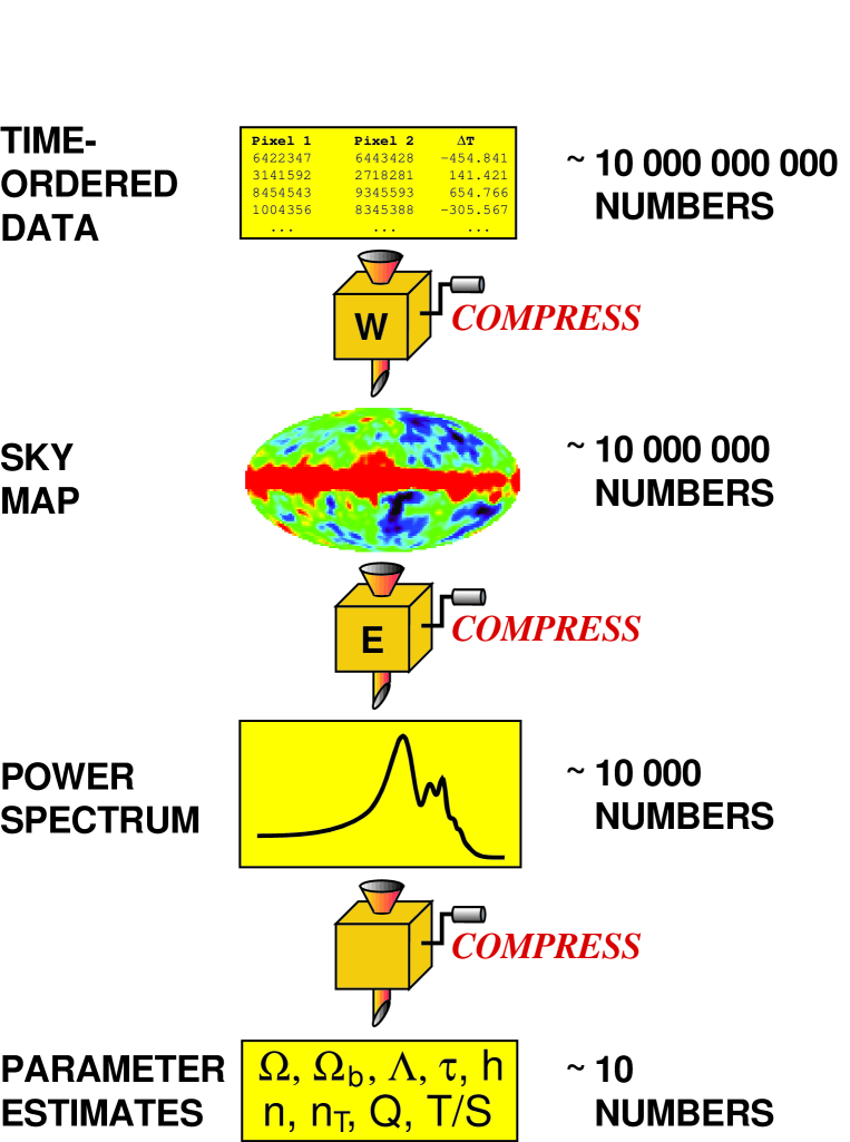
FIG. 1.: Power spectrum estimation as an intermediate data-compression step in converting the raw data from a future megapixel experiment to measurements of cosmological parameters. If all three data compression steps are lossless, then this data analysis pipeline will measure the parameters with just as small error bars as a (computationally unfeasible) likelihood analysis measuring the parameters directly from the time-ordered data.

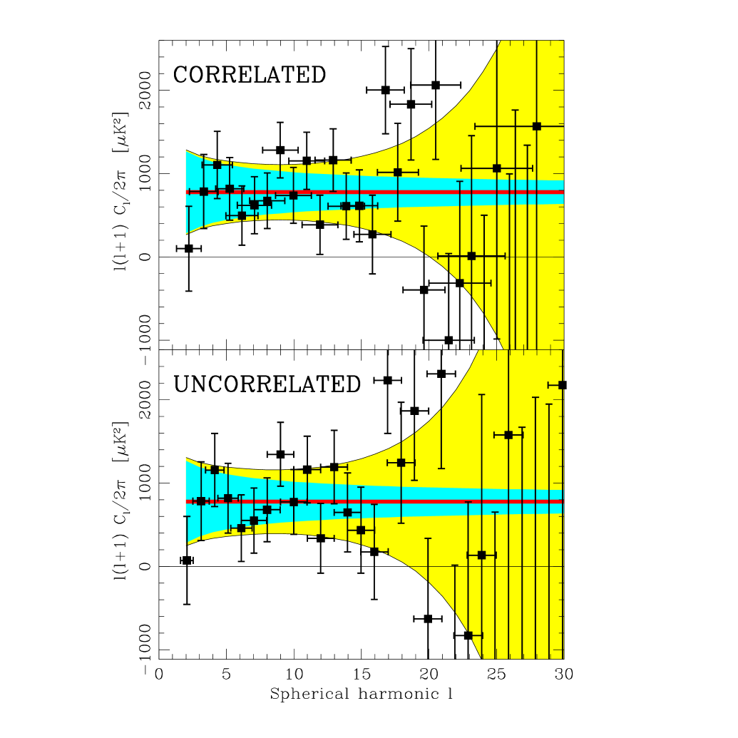
FIG. 2.: The power spectrum estimated from the COBE/DMR 4 year data.

The observed multipoles $D_{\l}=\l(\l+1)C_{\l}$ are plotted with $1-\sigma$ error bars using our basic method (top) and made uncorrelated with the ${\bf F}^{1/2}$-method of Section V A 6 (bottom). The vertical error bars include both pixel noise and cosmic variance, and the horizontal bars show the width of the window functions used. If the true power spectrum is given by $n=1$ and $Q_{rms,ps}=18.4{\rm\mu K}$ (the heavy horizontal line), then the shaded region gives the $1-\sigma$ error bars and the dark-shaded region shows the contribution from cosmic variance.

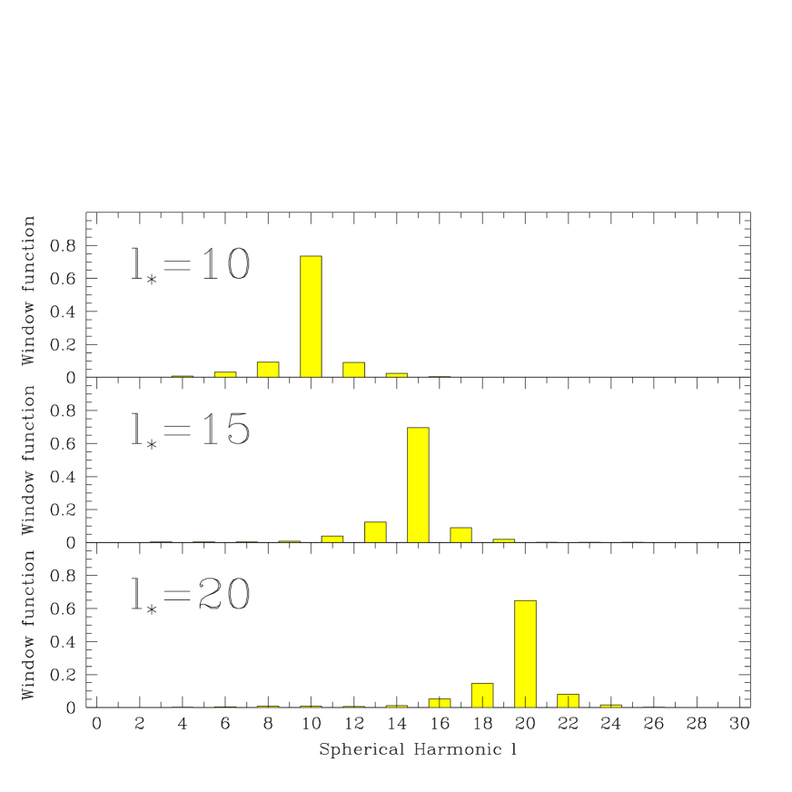
FIG. 3.: How the window functions depend on the target multipole.

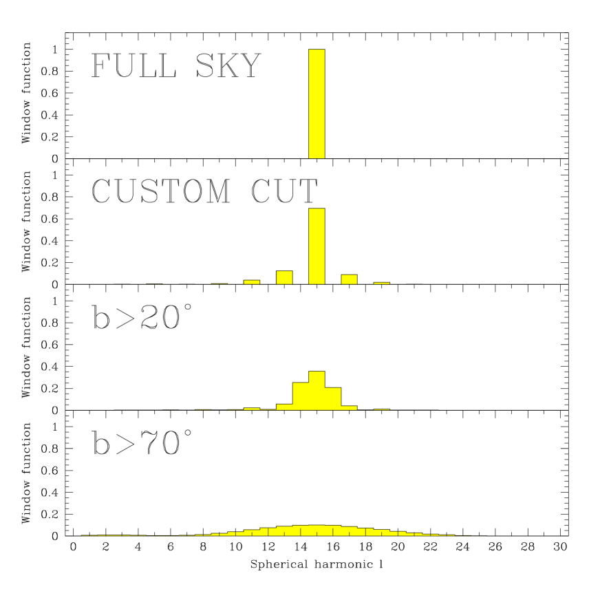
FIG. 4.: How the window functions depend on the sky coverage.

As the sky coverage decreases, the window function widens from a Kronecker delta to have a width $\Delta\l\sim 1/\Delta\theta$. In addition, since the custom cut is almost symmetric, it approximately preserves the orthogonality of even and odd multipoles.

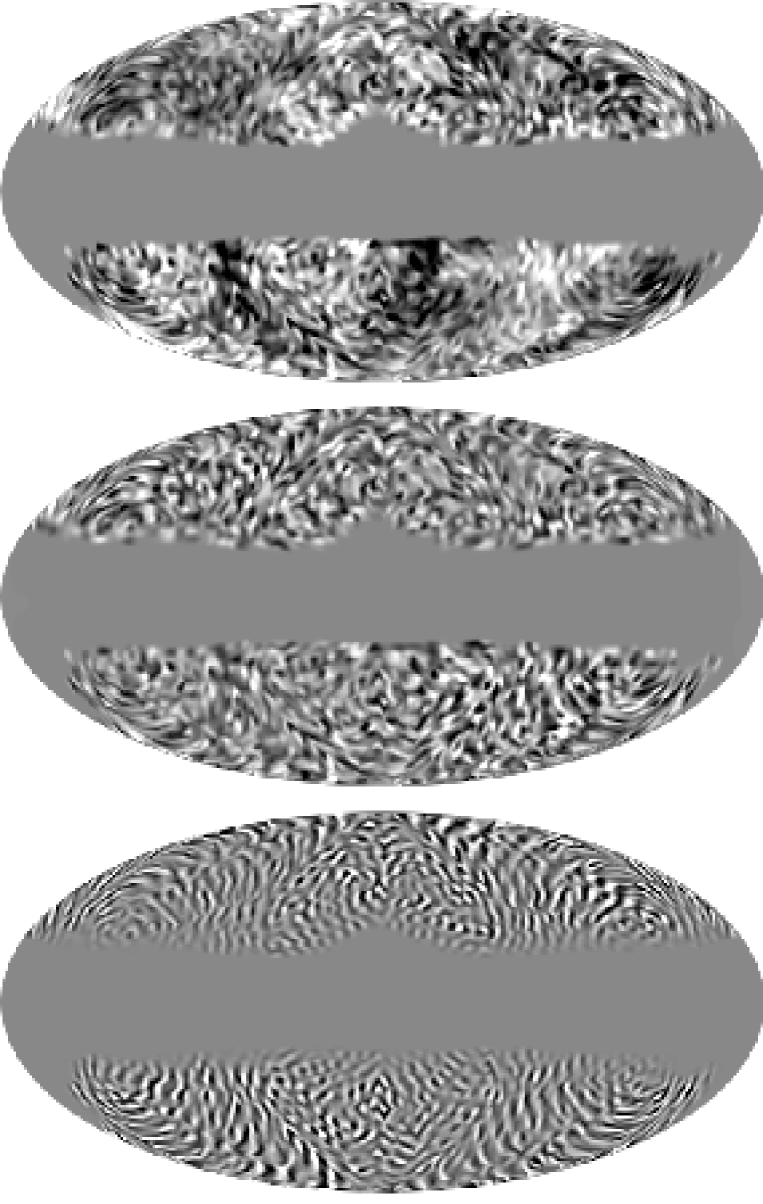
FIG. 5.: Sky maps before and after power tilting.

The 4-year COBE/DMR data (top) is shown after multiplication by the inverse pixel covariance matrix corresponding to the actual noise level (middle) and corresponding to the noise-level projected for Planck (bottom).

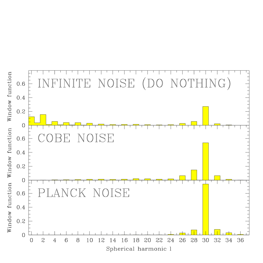
FIG. 6.: Window functions before and after power tilting.

Same as the previous figure, but in the Fourier (multipole) domain, showing the corresponding window functions for $\l_{*}=30$.

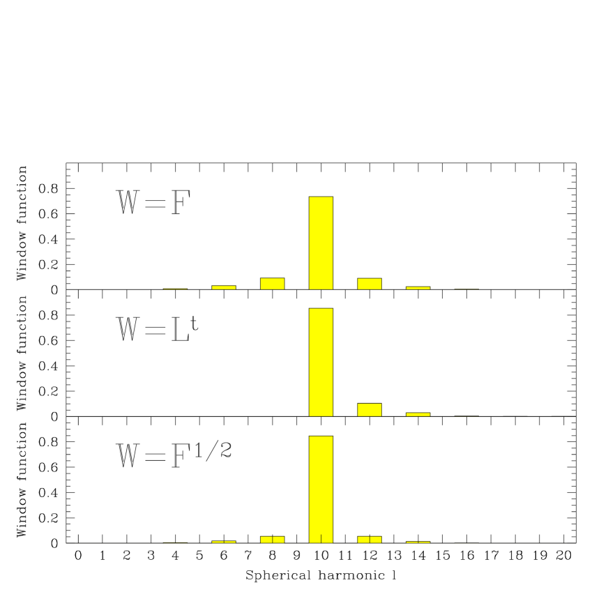
FIG. 7.: The $\l_{*}=10$ window functions for three of the data-presentation methods discussed, corresponding to using the original ${\bf y}$, Cholesky decomposing the Fisher matrix (${\bf F}=\L\L^{t}$) and taking its square root, respectively.

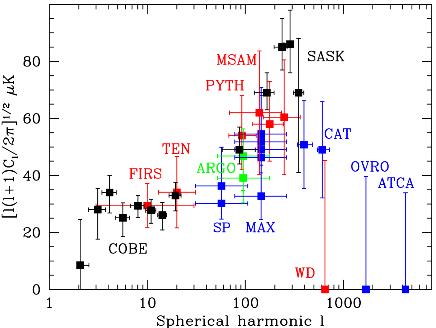
FIG. 8.: The power spectrum observed by COBE/DMR binned into 8 bands and compared with other experiments.

REFERENCES

- [1] G. Jungman, M. Kamionkowski, A. Kosowsky, and D. N. Spergel, Phys. Rev. Lett. 76, 1007 (1996).
- [2] G. Jungman, M. Kamionkowski, A. Kosowsky, and D. N. Spergel, Phys. Rev. D 54, 1332 (1996).
- [3] J. R. Bond, G. Efstathiou, and M. Tegmark, in preparation.
- [4] M. White, D. Scott, and J. Silk, ARA&A 32, 319 (1994).
- [5] W. Hu, N. Sugiyama, and J. Silk, preprint astro-ph/9604166.
- [6] J. R. Bond, Phys. Rev. Lett. 74, 4369 (1995).
- [7] E. F. Bunn and N. Sugiyama, ApJ 446, 49 (1995).
- [8] E. F. Bunn, Ph.D. Thesis, U.C. Berkeley (1995), ftp pac2.berkeley.edu/pub/bunn.
- [9] M. Tegmark, A. N. Taylor, and A. F. Heavens, ApJ, in press, preprint astro-ph/9603021 (1997).
- [10] M. Tegmark and E. F. Bunn, ApJ 455, 1 (1995).
- [11] G. Hinshaw et al., ApJL 464, L17 (1996).
- [12] M. Tegmark, preprint astro-ph/961113.
- [13] M. Tegmark, MNRAS 280, 299 (1996).
- [14] E. F. Bunn and M. White, preprint astro-ph/9607060.
- [15] A. J. S. Hamilton, preprint astro-ph/9701008, MNRAS, in press.
- [16] A. J. S. Hamilton, preprint astro-ph/9701009, MNRAS, in press.
- [17] C. L. Bennett et al., ApJ 464, L1 (1996).
- [18] M. Tegmark, ApJL 464, L35 (1996).
- [19] E. L. Wright et al., ApJ 420, 1 (1994).
- [20] M. G. Hauser and P. J. E. Peebles, ApJ 185, 757 (1973).
- [21] E. L. Wright et al., ApJ 436, 443 (1994).
- [22] E. L. Wright et al., ApJ 464, L21 (1996).
- [23] W. H. Press, B. P. Flannery, S. A. Teukolski, and W. T. Vetterling, Numerical Recipes, 2nd ed. (Cambridge Univ. Press, New York, 1992)
- [24] M. Tegmark & A. J. S. Hamilton, preprint astro-ph/9702019 (1997).
- [25] C. Lineweaver et al., preprint astro-ph/9610133 (1997).
- [26] G. Rocha & S. Hancock, preprint astro-ph/9611228 (1997).
- [27] E. L. Wright, G. Hinshaw, and C. L. Bennett, ApJL 458, L53 (1996).