Radiative Torques on Interstellar Grains:
II. Grain Alignment

Abstract

Radiative torques on irregular dust grains, in addition to producing superthermal rotation, play a direct dynamical role in the alignment of interstellar dust with the local magnetic field. The equations governing the orientation of spinning, precessing grains are derived; ${\rm H}_{2}$ formation torques and paramagnetic dissipation are included in the dynamics. Stationary solutions (constant alignment angle and spin rate) are found; these solutions may be stable (“attractors”) or unstable (“repellors”). The equations of motion are numerically integrated for three exemplary irregular grain geometries, exposed to anisotropic radiation with the spectrum of interstellar starlight. The resulting “trajectory maps” are classified as “noncyclic”, “semicyclic”, or “cyclic”, with examples of each given.

We find that radiative torques result in rapid grain alignment, even in the absence of paramagnetic dissipation. It appears that radiative torques due to starlight can account for the observed alignment of interstellar grains with the Galactic magnetic field.

1 Introduction

The discovery of the polarization of starlight (Hall 1949; Hall & Mikesell 1949; Hiltner 1949a,b) revealed not only that interstellar dust particles were nonspherical, but that some process had brought about large-scale alignment of these grains. The interstellar magnetic field was immediately suggested as a grain alignment agent possessing the large-scale coherence required by the polarization observations.

Initial investigations considered magnetic processes for bringing about the grain alignment. Both “compass-needle” alignment of ferromagnetic grains (Spitzer & Schatzman 1949; Spitzer & Tukey 1949, 1951) and paramagnetic dissipation in spinning grains (Davis & Greenstein 1949, 1950a,b, 1951) were initially proposed. When HI Zeeman splitting (Verschuur 1969) and dispersion and Faraday rotation toward pulsars (Woltjer 1970) indicated interstellar field strengths of 3-4$\mu$G, it was evident that “compass-needle” alignment was negligible, but paramagnetic dissipation on the Davis-Greenstein timescale $\tau_{\rm DG}$ [see eq.(19) below] appeared to be viable, particularly if the grains were superparamagnetic (Jones & Spitzer 1967). However, study of the statistical mechanics of grain alignment (Jones & Spitzer 1967; Purcell & Spitzer 1971) raised questions about the ability of the interstellar magnetic field to achieve the observed degree of grain alignment, since random gas-grain collisions (and magnetic fluctuations within the grain) would tend to oppose the alignment process.

Martin (1971) pointed out that because of the Rowland effect, charged interstellar grains would have a substantial magnetic moment either parallel or antiparallel to the angular velocity; this magnetic moment ensured that precession of the grain angular momentum around the magnetic field would be sufficiently rapid that the observed interstellar grain alignment should always be either parallel or perpendicular to the magnetic field direction, regardless of the mechanism responsible for grain alignment. Thus the galactic magnetic field could lead to large-scale coherence in observed grain alignment, even if the magnetic field itself played no direct role in grain alignment. This conclusion was reinforced when Dolginov & Mytrophanov (1976) noted that the Barnett effect implied much larger magnetic moments for spinning grains, leading to even more rapid precession of ${\bf J}$ around ${\bf B}_{0}$.

A very important development occurred when Purcell (1975, 1979) pointed out that grains were subject to systematic torques which, in diffuse clouds, would result in grain rotation rates far in excess of those which had been previously assumed to result from simple thermal excitation by collisions with gas atoms. Purcell considered three sources of systematic torques: ${\rm H}_{2}$ formation at preferred sites on the grain surface, photoelectron emission following absorption of a UV photon, and variations in the “accommodation coefficient” over the grain surface; the ${\rm H}_{2}$ formation torques appeared to be most important. Purcell observed that if these torques were long-lived, then normal paramagnetic relaxation would gradually bring the grain angular momentum into alignment with the magnetic field. However, if the grain surface changes on time scales short compared to $\tau_{\rm DG}$, substantial grain alignment would not occur. Spitzer & McGlynn (1978) analyzed the “crossover” process when the grain’s rotation rate (in body coordinates) undergoes a reversal due to a change in sign of the “Purcell torque”, and obtained an estimate for the disalignment caused by frequent crossovers. Spitzer & McGlynn concluded that if the active sites for ${\rm H}_{2}$ formation were short-lived, the disorientation during crossovers was too great for grains to be aligned by ordinary paramagnetic dissipation. The crossover phenomenon has recently been reanalyzed by Lazarian & Draine (1997), who find that the disalignment per crossover can be (paradoxically) substantially suppressed by “Barnett effect fluctuations”, with the result that paramagnetic alignment could potentially explain the observed alignment of $a\lower 2.15277pt\hbox{$\;\buildrel>\over{\sim}\;$}0.1\mu{\rm m}$ grains, if no other systematic torques acted to change the grain alignment.

In a previous paper (Draine & Weingartner 1996a; hereinafter Paper I) we found that interstellar starlight exerts very substantial torques on irregular grains. These “radiative torques” drive extreme superthermal rotation in grains with the sizes ($a\approx 0.2\mu{\rm m}$) which must be aligned to account for the observed interstellar polarization. In addition, radiative torques can act to change the direction of the grain rotation, and must therefore play a role in the process of grain alignment. This paper is devoted to a study of this phenomenon.

The grain geometry and coordinate systems are introduced in §2. §3 discusses the torques acting on the grain due to the Barnett effect, gas drag, ${\rm H}_{2}$ formation, paramagnetic dissipation, and absorption and scattering of starlight.

In §4 we obtain the equations of motion after averaging over precession, and we discuss the stationary points and “crossover points” allowed by these equations. “Trajectory maps” showing the evolution of the grain orientation and rotational velocity are discussed in §5, where we show that three different classes of grain behavior are possible. Examples of each of the three classes of trajectory map are presented. In many cases radiative torques, together with magnetic precession of ${\bf J}$ around ${\bf B}_{0}$, rapidly bring about alignment of the grain angular momentum ${\bf J}$ with the magnetic field ${\bf B}_{0}$.

In §6 we summarize the behavior of our three exemplary grains as a function of the angle $\psi$ between the magnetic field ${\bf B}_{0}$ and the starlight anisotropy direction. Since the surface density of active sites for ${\rm H}_{2}$ formation is uncertain, we examine the sensitivity of our results to this quantity, and find that, for likely values, radiative torques are more important than paramagnetic dissipation for producing grain alignment. In some cases the radiative torques do not allow a stationary solution; even in this case the average alignment can be substantial. Our results are summarized in §7.

2 Grain Dynamics in a Magnetic Field

2.1 Grain Geometry

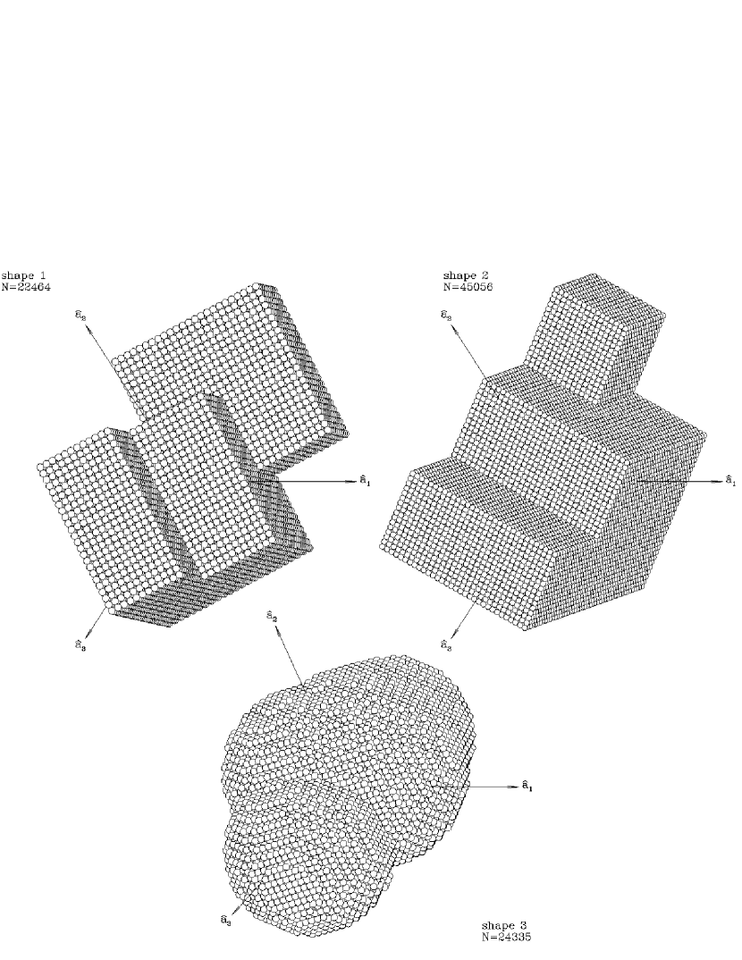
Figure 1: Three representative grain geometries. Shape 1 is the geometry studied in Paper I.

As in Paper I, we consider irregular grains of density $\rho$ and volume $V$, with an “effective radius” $a_{\rm eff}\equiv(3V/4\pi)^{1/3}=10^{-5}a_{-5}\,{\rm cm}$. In the present paper we report results for three specific grain shapes, shown in Fig. 1. Shape 1, which can be described as an assembly of 13 cubes, is the target geometry considered in Paper I. Shape 2 can be described as an assembly of 11 cubes, with coordinates given in Table 1. Shape 3 can be described as the union of 5 overlapping spheres, with coordinates and radii given in Table 2.

The moment of inertia tensor has eigenvalues $I_{1}\geq I_{2}\geq I_{3}$, with principal axes $\hat{\bf a}_{1}$, $\hat{\bf a}_{2}$, and $\hat{\bf a}_{3}$. We define dimensionless parameters $\alpha_{j}$ by

$$I_{j}\equiv\alpha_{j}{2\over 5}\rho Va_{\rm eff}^{2}~{}~{}~{}.$$ (1)

A sphere has $\alpha_{j}=1$; the irregular grain of Paper I has $\alpha_{1}=1.745$. In Table 3 we give $\alpha_{j}$ for shapes 2 and 3.

The thermal rotation rate for the grain is

$$\omega_{T}\equiv\left({15\over 8\pi\alpha_{1}}{kT\over\rho a^{5}}\right)^{1/2}=1.66\times 10^{5}\left(T\over 100{\rm K}\right)^{1/2}\left({3\,{\rm g}\,{\rm cm}^{-3}\over\rho}\right)^{1/2}\alpha_{1}^{-1/2}a_{-5}^{-2.5}\,{\rm s}^{-1}$$ (2)

for rotation around $\hat{\bf a}_{1}$ with kinetic energy $kT/2$.

2.2 Coordinate System

Consider unidirectional radiation, propagating in direction $\hat{\bf k}$. Without loss of generality we may choose the unit vectors $\hat{\bf e}_{1}$, $\hat{\bf e}_{2}$, $\hat{\bf e}_{3}$ defining the “scattering coordinates” such that $\hat{\bf e}_{1}$ is parallel to $\hat{\bf k}$, and the magnetic field ${\bf B}_{0}$ lies in the $\hat{\bf e}_{1},\hat{\bf e}_{2}$ plane (see Figures 2, 3). Let $\psi$ be the angle between ${\bf B}_{0}$ and $\hat{\bf k}$; since the sign of $B_{0}$ does not affect the grain dynamics, we need only consider $\psi\in[0,\pi/2]$. Let the “alignment angle” $\xi\in[0,\pi]$ be the angle between the grain principal axis $\hat{\bf a}_{1}$ and ${\bf B}_{0}$. The superthermally-rotating grain will be spinning around $\hat{\bf a}_{1}$; because of the Barnett moment (see §3.1), the axis $\hat{\bf a}_{1}$ of the spinning grain will rapidly precess in a cone around ${\bf B}_{0}$, and it is convenient to define a “precession frame” using polar coordinates $(r,\xi,\phi)$ with ${\bf B}_{0}$ as the polar axis. Then $(\xi,\phi)$ corresponds to the direction of the grain axis $\hat{\bf a}_{1}$:

$$\hat{\bf a}_{1}=\hat{\bf e}_{1}(\cos\psi\cos\xi-\sin\psi\sin\xi\cos\phi)+\hat{\bf e}_{2}(\sin\psi\cos\xi+\cos\psi\sin\xi\cos\phi)+\hat{\bf e}_{3}\sin\xi\sin\phi~{}~{},~{}~{}$$ (3)

and unit vectors in the directions of increasing $\xi$ and $\phi$ are given by

$$\hat{{\hbox{\boldsym\char 24\relax}}}\! \!=\! \!-\hat{\bf e}_{1}(\sin\psi\cos\xi\cos\phi+\cos\psi\sin\xi)+\hat{\bf e}_{2}(\cos\psi\cos\xi\cos\phi-\sin\psi\sin\xi)+\hat{\bf e}_{3}\cos\xi\sin\phi~{},~{}~{}$$ (4)

$$\hat{{\hbox{\boldsym\char 30\relax}}}\! \!=\! \!\hat{\bf e}_{1}\sin\psi\sin\phi-\hat{\bf e}_{2}\cos\psi\sin\phi+\hat{\bf e}_{3}\cos\phi~{}~{}~{}~{}.$$ (5)

The orientation angles $\Theta$ and $\Phi$ in the scattering frame (see Fig. 2) can be determined from

$$\Theta(\xi,\phi)=\cos^{-1}\left[\cos\psi\cos\xi-\sin\psi\sin\xi\cos\phi\right]~{}~{}~{}~{},$$ (6)

$$\Phi(\xi,\phi)=2\tan^{-1}\left[{\sin\Theta-\sin\psi\cos\xi-\cos\psi\sin\xi\cos\phi\over\sin\xi\sin\phi}\right]~{}~{}~{}~{}.$$ (7)

The grain orientation is also determined by the angle $\beta$ measuring rotation of the grain around $\hat{\bf a}_{1}$ (see Paper I and Fig. 2). In the present study we will assume the grain to spin rapidly around $\hat{\bf a}_{1}$ (see below) and will therefore employ radiative torques obtained after averaging over angle $\beta$; henceforth, this angle will not be explicitly mentioned.

2.3 Grain Dynamics

When $\omega^{2}\gg\omega_{T}^{2}$, internal dissipation in the grain will tend to bring the principal axis of largest moment of inertia $\hat{\bf a}_{1}$ into alignment with the angular moment ${\bf J}$, as this is the state of minimum kinetic energy for fixed ${\bf J}$. As discussed by Purcell (1979), both viscoelasticity and Barnett relaxation are effective. In fact, thermal fluctuations will act to prevent perfect alignment of ${\bf J}$ with $\hat{\bf a}_{1}$ (Lazarian & Roberge 1997). In the analysis below we will assume perfect alignment of $\hat{\bf a}_{1}$ with ${\bf J}$, so that ${\hbox{\boldsym\char 33\relax}}=\omega\hat{\bf a}_{1}$. Then

$$I_{1}\left[\hat{\bf a}_{1}{d\omega\over dt}+\hat{{\hbox{\boldsym\char 24\relax}}}\omega{d\xi\over dt}+\hat{{\hbox{\boldsym\char 30\relax}}}\omega\sin\xi{d\phi\over dt}\right]={\bf\Gamma}_{\rm B}+{\bf\Gamma}_{rad}+{\bf\Gamma}_{{\rm H}_{2}}+{\bf\Gamma}_{drag}+{\bf\Gamma}_{\rm DG}~{}~{}~{}~{},$$ (8)

where ${\bf\Gamma}_{\rm B}$ is the torque due to the Barnett moment, ${\bf\Gamma}_{rad}$ is the radiative torque due to starlight, ${\bf\Gamma}_{{\rm H}_{2}}$ is the torque due to ${\rm H}_{2}$ formation, ${\bf\Gamma}_{drag}$ is the drag torque due to gas atoms (and photon emission), and ${\bf\Gamma}_{\rm DG}$ is the “Davis-Greenstein” torque due to paramagnetic dissipation. These torques are discussed below.

3 Torques

3.1 Barnett Moment and Precession around ${\bf B}_{0}$

Spinning grains develop a magnetic moment ¯ antiparallel to !, primarily due to the Barnett effect (Dolginov & Mytrophanov 1976); if the grain is charged there is a small correction due to the Rowland effect which we shall neglect. The Barnett magnetic moment is

$${\hbox{\boldsym\char 22\relax}}=-{\chi(0)V\hbar\over g\mu_{B}}{\hbox{\boldsym\char 33\relax}}~{}~{}~{}~{},$$ (9)

where $V$ is the grain volume, $\mu_{B}$ is the Bohr magneton, $g\approx 2$ is the gyromagnetic ratio, and $\chi(0)$ is the static susceptibility. The magnetic properties of interstellar grains have recently been reviewed by Draine (1996); “normal” paramagnetism is expected to result in $\chi(0)\approx 10^{-4}$, and superparamagnetism would give even larger values of $\chi(0)$.

The torque resulting from the Barnett effect magnetic moment is

$${\bf\Gamma}_{\rm B}={\hbox{\boldsym\char 22\relax}}\times{\bf B}_{0}=-\hat{{\hbox{\boldsym\char 30\relax}}}I_{1}\Omega_{\rm B}\omega\sin\xi~{}~{}~{}.$$ (10)

This torque will cause the grain to precess in the Galactic magnetic field ${\bf B}_{0}$ with a precession frequency

$$\Omega_{B}={\mu B_{0}\over I_{1}\omega}={5\hbar\chi(0)B_{0}\over 2\alpha_{1}g\mu_{B}\rho a_{\rm eff}^{2}}\approx 7.5{\rm yr}^{-1}a_{-5}^{-2}\left({3\,{\rm g}\,{\rm cm}^{-3}\over\alpha_{1}\rho}\right)^{1/2}\left({\chi(0)\over 10^{-4}}\right)\left({B_{0}\over 5\mu{\rm G}}\right)~{}~{}~{}~{},$$ (11)

where we have set $g\approx 2$. It is therefore clear that interstellar grains will precess around ${\bf B}_{0}$ very rapidly compared to all other timescales except the grain rotation period itself.

3.2 Gas Drag

The drag torque is

$${\bf\Gamma}_{drag}=-\hat{\bf a}_{1}~{}I_{1}~{}\omega~{}\tau_{drag}^{-1}~{}~{}~{},$$ (12)

where the timescale for gas drag is (Paper I)

$$\tau_{drag}={\pi~{}\alpha_{1}~{}\rho~{}a_{\rm eff}\over 3\delta n_{\rm H}(2\pi m_{\rm H}kT)^{1/2}}=8.74\times 10^{4}{\rm yr}{\alpha_{1}\over\delta}\left(\rho\over 3\,{\rm g}\,{\rm cm}^{-3}\right)~{}a_{-5}T_{2}^{1/2}\left({3000\,{\rm cm}^{-3}K\over n_{\rm H}T}\right)~{}~{}~{},$$ (13)

where the drag coefficient $\delta$ is of order unity. A sphere has $\delta=1$; we estimate $\delta\approx 2$ for shapes 1 and 2, and $\delta\approx 1.5$ for the more compact shape 3.

There is also drag on the grain due to emission of far-infrared radiation; while it can be comparable to gas drag for very small grains (Paper I), it is unimportant for the $a_{\rm eff}\approx 0.1\mu{\rm m}$ grains we shall be interested in here, so we shall neglect it.

3.3 H₂ Formation

Purcell (1979) estimated the torque due to ${\rm H}_{2}$ formation on the grain surface, after averaging over the grain rotation, to be

$${\bf\Gamma}_{{\rm H}_{2}}\cdot\hat{\bf a}_{1}={1\over 3}\left({\pi\over 3}\right)^{1/6}f~{}n({\rm H})~{}(2EkT)^{1/2}a_{\rm eff}^{2}~{}l~{}p(t)~{}~{}~{}.$$ (14)

where $l^{2}$ is the surface area per ${\rm H}_{2}$ formation site on the grain surface, $f$ is the fraction of the arriving H atoms which depart as ${\rm H}_{2}$, $E$ is the kinetic energy of the departing ${\rm H}_{2}$ molecules, and $p(t)$ is a random variable with time averages $\langle p(t)\rangle=0$, $\langle p(t)p(t+\tau)\rangle=e^{-\tau/t_{L}}$, where $t_{L}$ is the “lifetime” of a surface recombination site. We define a characteristic rotation rate

$$\omega_{{\rm H}_{2}} = {5\over 24}\left({3\over\pi}\right)^{1/3}{f\over\delta}\left({E\over 3m_{\rm H}}\right)^{1/2}\left({n({\rm H})\over n_{\rm H}}\right){l\over a_{\rm eff}^{2}}$$ (15)

$$\approx 5.20\times 10^{7}\,{\rm s}^{-1}{f\over\delta a_{-5}^{2}}\left({l\over 10\,{\rm\AA}}\right)\left({E\over 0.2\,{\rm eV}\,}\right)^{1/2}\left({n({\rm H})\over n_{\rm H}}\right)$$ (16)

such that the ${\rm H}_{2}$ torque, averaged over the grain rotation, is

$${\bf\Gamma}_{{\rm H}_{2}}=\hat{\bf a}_{1}{I_{1}\omega_{{\rm H}_{2}}\over\tau_{drag}}p(t)~{}~{}~{}.$$ (17)

Note that $\omega_{{\rm H}_{2}}$ is proportional to $l$, the characteristic separation between ${\rm H}_{2}$ formation sites. We will usually assume $l=10\,{\rm\AA}$ for purposes of illustration, but other values of $l$ will be considered below.

3.4 Paramagnetic Dissipation

Magnetic dissipation in the grain produces a torque (Davis & Greenstein 1951; Jones & Spitzer 1967)

$${\bf\Gamma}_{\rm DG}=-(\hat{{\hbox{\boldsym\char 24\relax}}}\sin\xi\cos\xi+\hat{\bf a}_{1}\sin^{2}\xi)I_{1}\omega~{}\tau_{\rm DG}^{-1}$$ (18)

where

$$\tau_{\rm DG}={2\alpha_{1}\rho a_{\rm eff}^{2}\over 5K(\omega)B_{0}^{2}}=1.5\times 10^{6}{\rm yr}~{}\left({\alpha_{1}\rho\over 3\,{\rm g}\,{\rm cm}^{3}}\right)a_{-5}^{2}\left({10^{-13}\,{\rm s}\over K(\omega)}\right)\left({5\mu{\rm G}\over B_{0}}\right)^{2}~{}~{}~{};$$ (19)

$K(\omega)\equiv\chi^{\prime\prime}(\omega)/\omega$, where $\chi^{\prime\prime}$ is the imaginary part of the complex susceptibility. We expect $K\approx 10^{-13}\,{\rm s}$ for normal paramagnetism and $\omega\lower 2.15277pt\hbox{$\;\buildrel<\over{\sim}\;$}10^{9}\,{\rm s}^{-1}$ (Jones & Spitzer 1967; Draine 1996).

3.5 Radiative Torques

As in Paper I, we approximate the interstellar radiation field in a diffuse cloud by an isotropic component with energy density $(1-\gamma)u_{rad}$ plus a unidirectional component with energy density $\gamma u_{rad}$. The radiative torque can be written (cf. Paper I)

$${\bf\Gamma}_{rad}(\xi,\phi)={u_{rad}a_{\rm eff}^{2}\bar{\lambda}\over 2}\left(\gamma\left[F(\xi,\phi)\hat{{\hbox{\boldsym\char 24\relax}}}+G(\xi,\phi)\hat{{\hbox{\boldsym\char 30\relax}}}+H(\xi,\phi)\hat{\bf a}_{1}\right]+(1-\gamma)\langle Q_{\Gamma}^{\rm iso}\rangle\hat{\bf a}_{1}\right)~{}~{}~{},$$ (20)

$$F(\xi,\phi) = \langle{\bf Q}_{\Gamma}\rangle\!\cdot\!\hat{\bf e}_{1}(-\sin\psi\cos\xi\cos\phi-\cos\psi\sin\xi)+$$ (21)

$$\langle{\bf Q}_{\Gamma}\rangle\!\cdot\!\hat{\bf e}_{2}(\cos\psi\cos\xi\cos\phi-\sin\xi\sin\psi)+\langle{\bf Q}_{\Gamma}\rangle\!\cdot\!\hat{\bf e}_{3}\cos\xi\sin\phi$$

$$G(\xi,\phi) = \langle{\bf Q}_{\Gamma}\rangle\!\cdot\!\hat{\bf e}_{1}\sin\psi\sin\phi-\langle{\bf Q}_{\Gamma}\rangle\!\cdot\!\hat{\bf e}_{2}\cos\psi\sin\phi+\langle{\bf Q}_{\Gamma}\rangle\!\cdot\!\hat{\bf e}_{3}\cos\phi$$ (22)

$$H(\xi,\phi) = \langle{\bf Q}_{\Gamma}\rangle\!\cdot\!\hat{\bf e}_{1}(\cos\psi\cos\xi-\sin\psi\sin\xi\cos\phi)+$$ (23)

$$\langle{\bf Q}_{\Gamma}\rangle\!\cdot\!\hat{\bf e}_{2}(\sin\psi\cos\xi+\cos\psi\sin\xi\cos\phi)+\langle{\bf Q}_{\Gamma}\rangle\!\cdot\!\hat{\bf e}_{3}\sin\xi\sin\phi$$

where the radiative torque efficiency vector ${\bf Q}_{\bf\Gamma}(\Theta,\Phi)$ depends on $\xi$, $\phi$, and the angle $\psi$ between ${\bf B}_{0}$ and ${\bf k}$, $Q_{\Gamma}^{\rm iso}$ is the torque efficiency factor for isotropic radiation, and $\langle\rangle$ denotes averaging over the incident radiation spectrum, here assumed to be the interstellar radiation field (“ISRF”) spectrum (Mezger, Mathis, & Panagia 1982; Mathis, Mezger, & Panagia 1983), for which $u_{rad}=8.64\times 10^{-13}\,{\rm ergs}\,{\rm cm}^{-3}$, $\bar{\lambda}=1.202\mu{\rm m}$. $\langle Q_{\Gamma}^{\rm iso}\rangle_{ISRF}$ is given in Table 4 for shapes 1–3; we see that it is only $\sim 1\%$ of $\hat{\bf a}_{1}\cdot\langle{\bf Q}_{\Gamma}\rangle_{ISRF}(\Theta=0)$, showing that the radiative torque due to isotropic starlight is negligible compared to that due to anisotropic starlight, unless the anisotropic component is less than $\sim 1\%$ of the total background. The angles $\Theta(\xi,\phi)$ and $\Phi(\xi,\phi)$ are obtained using eq. (6,7). The grains are assumed to be composed of material with the dielectric function of “astronomical silicate” (Draine & Lee 1984).

As discussed in Paper I, it is sufficient to compute only ${\bf Q}_{\Gamma}(\Theta,0)$. Expressions for $F$, $G$, and $H$ in terms of ${\bf Q}_{\Gamma}(\Theta,0)$ are given in the Appendix. ${\bf Q}_{\Gamma}(\Theta,0)$ was computed as described in Paper I, assuming $\Phi=0$ and a number of different values of the grain rotation angle $\beta$.

As discussed in Paper I, computation of ${\bf Q}_{\Gamma}(\Theta,0)$ as a function of both $\Theta$ and wavelength $\lambda$ is very cpu-intensive. Accordingly, we have considered only the three grain shapes of Fig. 1, and only a single size ($a_{\rm eff}=0.2\mu{\rm m}$) for each shape.

4 Grain Dynamics

4.1 Equations of Motion

From eq.(8) we obtain three equations of motion:

$${d\phi\over dt} = {\gamma u_{rad}\bar{\lambda}a_{\rm eff}^{2}\over 2I_{1}\omega\sin\xi}G(\xi,\phi)-\Omega_{\rm B}~{}~{}~{},$$ (24)

$${d\xi\over dt} = {\gamma u_{rad}\bar{\lambda}a_{\rm eff}^{2}\over 2I_{1}\omega}F(\xi,\phi)-{\sin\xi\cos\xi\over\tau_{\rm DG}}~{}~{}~{},$$ (25)

$${d\omega\over dt} = {u_{rad}\bar{\lambda}a_{\rm eff}^{2}\over 2I_{1}}\left[\gamma H(\xi,\phi)+(1-\gamma)\langle Q_{\Gamma}^{\rm iso}\rangle\right]-{\omega\sin^{2}\xi\over\tau_{\rm DG}}+{\omega_{{\rm H}_{2}}p(t)\over\tau_{drag}}-{\omega\over\tau_{drag}}~{}~{}~{}.$$ (26)

Because the precession rate $\Omega_{\rm B}$ [see eq.(11)] is so much faster than the other terms in eq.(24-26) we may immediately average over $\phi$ in eq.(25,26):

$${d\xi\over dt^{\prime}} \approx {\gamma{M}\over\omega^{\prime}}\bar{F}(\xi)-\beta\sin\xi\cos\xi~{}~{}~{},$$ (27)

$${d\omega^{\prime}\over dt^{\prime}} \approx {M}\left[\gamma\bar{H}(\xi)+(1-\gamma)\langle Q_{\Gamma}^{\rm iso}\rangle\right]+\eta p(t)-\left(1+\beta\sin^{2}\xi\right)\omega^{\prime}~{}~{}~{},$$ (28)

where $t^{\prime}\equiv t/\tau_{drag}~{}$, $~{}~{}~{}\omega^{\prime}\equiv\omega/\omega_{T}~{}$, and

$$\beta \equiv {\tau_{drag}\over\tau_{\rm DG}}~{}~{}~{},$$ (29)

$$\eta \equiv {\omega_{{\rm H}_{2}}\over\omega_{T}}~{}~{}~{},$$ (30)

$${M} \equiv {u_{rad}\bar{\lambda}a_{\rm eff}^{2}\tau_{drag}\over 2I_{1}\omega_{T}}={6.83\times 10^{4}\over\delta}\left({u_{rad}\over n_{\rm H}kT}\right)\left({\bar{\lambda}\over\mu{\rm m}}\right)\left({\alpha_{1}\rho a_{-5}\over 3\,{\rm g}\,{\rm cm}^{-3}}\right)^{1/2}~{}~{}~{}~{},$$ (31)

$$\bar{F}(\xi) \equiv {1\over 2\pi}\int_{0}^{2\pi}F(\xi,\phi)d\phi~{}~{}~{}~{},~{}~{}~{}~{}~{}~{}~{}\bar{H}(\xi)\equiv{1\over 2\pi}\int_{0}^{2\pi}H(\xi,\phi)d\phi~{}~{}~{}~{}.$$ (32)

[Note that the parameter $\beta$ in eq. (29) is not to be confused with the angle $\beta$ in Fig. 2.] For the numerical examples in this paper, we assume conditions appropriate to an interstellar diffuse cloud: $n_{\rm H}=30\,{\rm cm}^{-3}$, $n({\rm H})/n_{\rm H}=1$, $T=100{\rm K}$, $B=5\mu{\rm G}$. We consider a grain of silicate composition with $\rho=3\,{\rm g}\,{\rm cm}^{-3}$, $K=10^{-13}\,{\rm s}$, and $a_{-5}=2$. For most examples we assume $f=1/3$, $l=10\,{\rm\AA}$, and $E=0.2\,{\rm eV}\,$. Thus

$$\beta = 2.87\times 10^{-2}\left({2\over\delta}\right)~{}~{}~{}~{},$$ (33)

$$\eta = 272\left({\alpha_{1}\over 1.5}\right)^{1/2}\left({2\over\delta}\right)f\left({l\over 10\,{\rm\AA}}\right)~{}~{}~{}~{},$$ (34)

$${M} = 1.49\times 10^{5}\left({\alpha_{1}\over 1.5}\right)^{1/2}\left({2\over\delta}\right)~{}~{}~{}~{}.$$ (35)

The functions $\bar{F}(\xi)$ and $\bar{H}(\xi)$ are plotted in Figures 4 and 5 for shape 1, $a_{\rm eff}=0.2\mu{\rm m}$, and the interstellar radiation field.

4.2 Stationary Points

Because $p(t)$ in eq. (14,17,26,28) fluctuates, there are no true steady-state solutions. If the surface site lifetime $t_{L}\gg\tau_{drag}$, then there will be quasi-steady solutions $\xi_{s}(p)$, $\omega_{s}(p)$; $\xi_{s}$ is a zero of the function

$$Z(\xi)\equiv\bar{F}(\xi)-{\beta\sin\xi\cos\xi\over 1+\beta\sin^{2}\xi}\left[\gamma\bar{H}(\xi)+(1-\gamma)\langle Q_{\Gamma}^{\rm iso}\rangle+{\eta p\over{M}}\right]~{}~{}~{}~{},$$ (36)

and $\omega_{s}$ is given by

$$\omega_{s}^{\prime}={\omega_{s}\over\omega_{T}}={{M}\left[\gamma\bar{H}(\xi_{s})+(1-\gamma)\langle Q_{\Gamma}^{\rm iso}\rangle\right]+\eta p\over 1+\beta\sin^{2}\xi_{s}}~{}~{}~{}~{}.$$ (37)

From Figs. 4 and 5 we see that $\bar{F}$ and $\bar{H}$ are of comparable magnitude. Since for conditions of interest we have $\gamma\approx 0.1$, $M\gg 1$, and $\beta\ll 1$ (see eq. 31,33), it is apparent from eq. (36) that $Z(\xi)\approx\bar{F}(\xi)$, so that the zeros of $Z$ will nearly coincide with the zeros of $\bar{F}$. The ${\rm H}_{2}$ torques and Davis-Greenstein torques have only a minimal effect on the function $Z(\xi)$, and hence on the angles $\xi_{s}$ for stationary solutions (although the angular velocities $\omega_{s}$ are significantly dependent on the ${\rm H}_{2}$ torques, as will be seen below).

The timescale for approach to alignment angle $\xi_{s}$ may be estimated by linearizing eq. (27,28) around $(\xi_{s},\omega_{s})$:

$${d\xi\over dt^{\prime}} \approx A(\xi-\xi_{s})+B(\omega^{\prime}-\omega_{s}^{\prime})~{}~{}~{},$$ (38)

$${d\omega^{\prime}\over dt^{\prime}} \approx C(\xi-\xi_{s})+D(\omega^{\prime}-\omega_{s}^{\prime})~{}~{}~{},$$ (39)

where

$$A = {\gamma{M}\over\omega_{s}^{\prime}}{d\bar{F}\over d\xi}-\beta\cos 2\xi_{s}~{}~{}~{},$$ (40)

$$B = -{\gamma{M}\over(\omega_{s}^{\prime})^{2}}\bar{F}(\xi_{s})~{}~{}~{},$$ (41)

$$C = \gamma{M}{d\bar{H}\over d\xi}-\beta\omega_{s}^{\prime}\sin 2\xi_{s}~{}~{}~{},$$ (42)

$$D = -\left(1+\beta\sin^{2}\xi_{s}\right)~{}~{}~{}.$$ (43)

The stationary point $(\xi_{s},\omega_{s})$ is an attractor (i.e., stable) provided both

$$A+D<0~{}~{}~{}~{}~{}{\rm and}~{}~{}~{}~{}~{}BC-AD<0~{}~{}~{};$$ (44)

otherwise it is a repellor (i.e., unstable). If stable, there will be two relaxation times for approach to the stationary point, given by

$$\tau_{relax}^{-1}={-(A+D)\pm\left[(A-D)^{2}+4BC\right]^{1/2}\over 2\tau_{drag}}~{}~{}~{}.$$ (45)

We take the slower of these two relaxation rates to give the alignment time:

$$\tau_{align}^{-1}={-(A+D)-\left[(A-D)^{2}+4BC\right]^{1/2}\over 2\tau_{drag}}~{}~{}~{}.$$ (46)

4.3 Crossover Points

When $\omega\rightarrow 0$, eq.(27) is singular unless $\bar{F}=0$. Therefore $\omega$ can only change sign at a crossover point $\xi_{c}$ where

$$\bar{F}(\xi_{c})=0~{}~{}~{}~{}.$$ (47)

From eq.(21) and eq.(32) it is easily seen that $\xi_{c}=0,\pi$ are always solutions to eq.(47). The crossover point acts as an attractor if

$${\gamma M\over M[\gamma\bar{H}(\xi_{c})+(1-\gamma)\langle Q_{\Gamma}^{\rm iso}\rangle]+\eta p}\left({d\bar{F}\over d\xi}\right)>0~{}~{}~{}~{},$$ (48)

and as a repellor if eq.(48) is not satisfied. Physical “crossovers” will only occur at crossover points which are attractors.

We define the “polarity” of a crossover point as positive or negative according to the sign of $d\omega/dt$. From eq.(28) we see that

$${\rm polarity}~{}={\rm sign}\left\{M[\gamma\bar{H}(\xi_{c})+(1-\gamma)\langle Q_{\Gamma}^{\rm iso}\rangle]+\eta p\right\}~{}~{}~{}~{}.$$ (49)

5 Trajectory Maps

5.1 Map Classification

Provided the rotation is highly superthermal (so that we may assume that $\hat{\bf a}_{1}\parallel{\bf J}/\omega$), and rotation and precession are both rapid compared to the timescale for changes in $\omega$ or $\xi$, the grain state is specified by two coordinates: the angle $\xi$ between ${\bf J}$ and ${\bf B}_{0}$, and the rate $\omega$ of rotation around $\hat{\bf a}_{1}$. The dynamical evolution of the grain therefore corresponds to a trajectory on the $\xi,\omega$ plane. Each point on the $\xi,\omega$ plane lies on a single trajectory, except for (1) stationary attractors where many different trajectories have a common end point, or (2) crossover attractors, where many different trajectories converge.

We refer to the set of all trajectories as the “trajectory map”. The $\xi,\omega$ plane naturally separates into two regions, $\omega>0$ and $\omega<0$, with trajectories connecting the regions only at a small number of crossover attractors (a crossover repellor formally admits a single trajectory connecting the two regions but this is a set of zero area on the $\xi,\omega$ plane). To a considerable extent it is possible to classify trajectory maps according to the types of stationary points and crossover points which they possess. Three distinct types of trajectory maps are possible.

5.1.1 Cyclic Maps

If a trajectory map has no stationary attractors, then the generic trajectory does not end. Such trajectory maps are referred to as “cyclic”. Fig. 8 is an example of a cyclic map.

From eq.(27) we see that if $\beta=0$ (i.e., $\tau_{\rm DG}\rightarrow\infty$: no Davis-Greenstein torque), then the sign of $d\xi/dt$ is independent of $\omega$ (except for the sign of $\omega$). Since a closed trajectory must have two points with the same $\xi$ but opposite signs of $d\xi/dt$, it follows that there can be no closed trajectories contained within either the $\omega>0$ or $\omega<0$ regions. If closed trajectories exist, then each such trajectory must pass through $\omega=0$ at an even number of crossover attractors, and the trajectory must have equal numbers of crossover attractors of positive and negative polarity (usually just one of each).

For finite $\tau_{\rm DG}$ closed trajectories which do not cross $\omega=0$ could, in principle, exist, depending on the properties of $\bar{F}(\xi)$ and $\bar{H}(\xi)$ (although any such trajectories cannot cross $\xi=0$). However, since $\beta\ll 1$ for interstellar conditions of interest, it seems safe to assume that closed trajectories do not occur unless they cross $\omega=0$. This will henceforth be assumed.

5.1.2 Noncyclic Maps

If the trajectory map does not have at least one crossover attractor of each parity then, following the discussion above, there will be no closed trajectories. We refer to this type of map as “noncyclic”.

In a noncyclic map, every trajectory must terminate at a stationary attractor point, on a timescale given by eq. (46); thus there must be at least one stationary attractor. Figs. 9 – 11 are examples of noncyclic trajectory maps.

5.1.3 Semicyclic Maps

The case where there are both closed trajectories but also at least one stationary attractor will be referred to as “semicyclic”. A necessary condition for a semicyclic map is that there be at least one crossover attractor of each polarity, and at least one stationary attractor. If there is no crossover repellor situated between two crossover attractors of opposite polarity, then there will be trajectories with $|\omega|\rightarrow 0$ connecting the two crossover attractors. Therefore a sufficient condition for a semicyclic map is that there be at least one stationary attractor, and at least one pair of crossover attractors of opposite parity with no crossover repellor in between. Figs. 6 and 7 are examples of semicyclic maps.

If there is a repellor situated between each pair of opposite-polarity crossover attractors, there may be no closed trajectories: Fig. 11 is an example of such a noncyclic trajectory map. We conjecture that whenever a crossover repellor lies between each pair of opposite-polarity crossover attractors, the trajectory map will be noncyclic.

5.2 Examples

In Figure 6 we show evolutionary trajectories for an $a_{\rm eff}=0.2\mu{\rm m}$ silicate grain with the geometry of shape 1 in Fig. 1, for $\psi=0$ (anisotropic component of the radiation field parallel to ${\bf B}_{0}$). We show results assuming $p=0$ (no ${\rm H}_{2}$ torques) and $\tau_{\rm DG}=\infty$ (no Davis-Greenstein torque): the only torques are due to gas drag and starlight. This is an example of a semicyclic map. The arrows in the figure are at intervals of $0.5t_{drag}=7.5\times 10^{4}{\rm yr}$. We see that trajectories beginning at $\omega>0$ all converge on the crossover point at $\cos\xi=-.873$, where they enter the region $\omega<0$. Some of the trajectories in the region $\omega<0$ evolve to the stationary attractor at $\cos\xi=-1$; others lead to the crossover attractor at $\cos\xi=1$, where they enter the $\omega>0$ region.

As mentioned above, in our analysis the crossover points are singular – we are unable to follow a grain’s evolution through the crossover event, and therefore we cannot predict which of the trajectories emerging from a crossover attractor will be “populated”. Furthermore, our analysis assumes superthermal rotation with perfect Barnett relaxation so that $\hat{\bf a}_{1}\parallel{\bf J}/\omega$. This approximation will be accurate when the grain rotation is extremely superthermal, $(\omega/\omega_{T})^{2}\gg 1$, but fails when the rotational kinetic energy approaches thermal values. The region $(\omega/\omega_{T})^{2}<10$ is shaded in Figs. 6-10; with our present approximations we are unable to follow trajectories within this region.

If we now include ${\rm H}_{2}$ formation torques (with $p=+1$) and Davis-Greenstein torques due to normal paramagnetism ($\tau_{\rm DG}=1.0\times 10^{7}{\rm yr}$) the “flow pattern” changes to that shown in Figure 7. The map remains semicyclic. Figures 6 and 7 are qualitatively similar, showing that ${\rm H}_{2}$ torques, while by no means negligible, appear to be of secondary importance compared to radiative torques for $a_{\rm eff}=0.2\mu{\rm m}$ grains.

Figures 6 and 7 each show semicyclic behavior. Some trajectories (e.g., from $\omega=-300\omega_{T}$ and $\cos\xi=-.9$) proceed directly to a stable attractor where they are captured. Other trajectories (e.g., from $\omega=-300\omega_{T}$, $\cos\xi=-.8$) head for the crossover attractor. In Figures 6 and 7 it is clear that even though we are unable to predict how the grain will emerge from the crossover point at $\cos\xi=1$, we know that the grain must then proceed to the other crossover attractor at $\cos\xi=-.88$. At this crossover the details matter: some trajectories emerging from the crossover lead to the stable attractor, while other trajectories return to the crossover point at $\cos\xi=+1$. In principle, it is possible that a grain could cycle back and forth between these two crossover points many times; it then becomes essential to understand the mechanics (and statistics) of the crossover process. Such cyclic behavior will in general be a possibility whenever we have two crossover attractors of opposite polarity with no crossover repellor in between.

Figure 8 shows the trajectory map for the same grain as in Figure 7, but now for an angle $\psi=30\arcdeg$ between ${\bf B}_{0}$ and the starlight anisotropy. We now have two stationary points rather than three, and there are no stationary attractors: the grain must continuously cycle between the two crossover attractors, which again have opposite polarity. This is a clear example of a “cyclic” trajectory map.

If we rotate the anisotropy direction to $\psi=60\arcdeg$ (Fig. 9) the stationary point at $\cos\xi=-1$ (which for $\psi=30\arcdeg$ was a repellor) crosses over into the $\omega>0$ region and becomes a stable attractor. The trajectory map now has a straightforward structure: there is only one stable attractor and only one stable crossover. The grain must evolve to the $\omega>0$ region, where it is inevitably trapped by the stable attractor.

The case $\psi=90\arcdeg$ (Fig. 10) shows new possibilities. Because of the symmetry of the problem, this trajectory map is symmetric under reflection through $\cos\xi=0$. There are five stationary points: two stationary attractors plus three stationary repellors. There are three crossover attractors, at $\cos\xi=\pm 1$ and 0; all have positive polarity. All trajectories lead to a stable attractor with $\cos^{2}\xi=0.514$. This is another example of a noncyclic trajectory map.

Finally, to illustrate the diversity of possible behaviors, Fig. 11 shows the trajectory map for an $a_{\rm eff}=0.2\mu{\rm m}$ silicate grain with the geometry of shape 3 (see Fig. 1) for an angle $\psi=0$ between the starlight anisotropy direction and ${\bf B}_{0}$. For this case there are four stationary points, three of which are attractors. There are two crossover attractors and three crossover repellors. This is a noncyclic map, but which of the three stationary attractors the grain is captured by depends on the initial conditions and (for trajectories which pass through the crossover attractor at $\xi=130\arcdeg$) on the details of the crossover process, which will determine which trajectories emerging from the crossover attractor are populated.

6 Discussion

6.1 Grain Alignment

It is by now evident that radiative torques lead to complex grain dynamics, which depend delicately on the grain geometry, the angle $\psi$ between the starlight anisotropy and the magnetic field ${\bf B}_{0}$, and on the ${\rm H}_{2}$ formation torque to which the grain is subject.

In the Rayleigh limit, the linear dichroism of a population of identical grains, each spinning around its axis $\hat{\bf a}_{1}$, is proportional to (see, e.g., Lee & Draine 1985)

$$\Delta\kappa=\langle R\rangle\sin^{2}\theta_{B}~{}n_{gr}\pi a_{\rm eff}^{2}Q_{pol}(\lambda)$$ (50)

where $\theta_{B}$ is the angle between ${\bf B}_{0}$ and the line-of-sight, $\langle R\rangle$ is the ensemble-averaged alignment parameter (or “Rayleigh reduction factor”)

$$R(\xi)\equiv{3\over 2}\left(\cos^{2}\xi-{1\over 3}\right)$$ (51)

and the polarization efficiency factor

$$Q_{pol}(\lambda) \equiv {1\over 2}\left[Q_{ext}({\bf E}\parallel\hat{\bf a}_{2},\hat{\bf k}\parallel\hat{\bf a}_{3})+Q_{ext}({\bf E}\parallel\hat{\bf a}_{3},\hat{\bf k}\parallel\hat{\bf a}_{2})-\right.$$ (52)

$$\left.~{}~{}~{}~{}Q_{ext}({\bf E}\parallel\hat{\bf a}_{1},\hat{\bf k}\parallel\hat{\bf a}_{2})-Q_{ext}({\bf E}\parallel\hat{\bf a}_{1},\hat{\bf k}\parallel\hat{\bf a}_{3})\right]~{}~{}~{},$$

where $Q_{ext}$ is the extinction efficiency factor for the grain. While eq. (50) for the linear dichroism is strictly valid only in the Rayleigh limit (where, of course, $Q_{ext}$ depends only on the direction of ${\bf E}$, but not on $\hat{\bf k}$) it provides a good approximation even when the grain is not small compared to the wavelength. Hence $\langle R\rangle$ is a useful statistic to characterize the effectiveness of grain alignment.

Above we have shown 6 examples of trajectory maps, but these are obviously a very incomplete sampling of parameter space. To provide a more global picture of the grain dynamics, Figures 12–14 show the “terminal” values of the grain rotation rate $\omega$ and $\cos\xi$. The domains of noncylic, cyclic, and semicyclic solutions are indicated. The region labelled “noncyclic?” is where there is at least one stationary attractor, and there are crossover attractors of opposite polarity, but where each opposite polarity pair of crossover attractors has an intervening crossover repellor. As discussed above, we suspect that such cases are noncyclic, but we have not verified this in all cases.

In Figs. 12–14 the horizontal broken lines show the values of $\cos\xi=\pm 1/\surd 3=\pm 0.577$ corresponding to alignment parameter $R=0$. Solutions with $-0.577<\cos\xi<0.577$ are “antialigned”, with $R<0$, but it is apparent that antialigned stationary solutions are relatively rare. For example, Fig. 12 shows that for $p=1$ and $p=0$, shape 1 is antialigned only for $\psi=84^{\circ}$; even in this case the antialignment is minimal and there are competing stationary solutions with substantial alignment.

From visual inspection of Figures 12–14, we conclude that in a substantial fraction of cases, the grains have noncyclic trajectory maps with stationary solutions with appreciable, and often perfect, alignment.

6.2 Sensitivity to the Magnitude of the H₂ Formation Torque

The numerical examples considered above assume the characteristic separation between ${\rm H}_{2}$ formation sites to be $l=10\,{\rm\AA}$, with the ${\rm H}_{2}$ formation torque given by eq. 14 with $p=0,\pm 1$. It is quite possible that the surface density of active sites is lower ($l>10\,{\rm\AA}$), in which case the r.m.s. ${\rm H}_{2}$ torque will be larger. To explore this, we consider shape 3 with $a=0.2\mu{\rm m}$. In Figure 15 we show the stationary solutions for $pl=\pm 30,50,100\,{\rm\AA}$. For $|pl|\lower 2.15277pt\hbox{$\;\buildrel>\over{\sim}\;$}20\,{\rm\AA}$ the ${\rm H}_{2}$ formation torque dominates the grain spinup, and we no longer have cyclic trajectories (all crossovers have the same polarity). However, we still have multiple stationary points in many cases. The values of $R$ for these cases do not appear to be very sensitive to the value of $pl$. Furthermore, even though the ${\rm H}_{2}$ formation torques may dominate radiative torques in driving superthermal rotation, radiative torques may still be more important than Davis-Greenstein torques in bringing about alignment of the grain angular momentum with ${\bf B}_{0}$. This is evident in Figure 16, showing the alignment time as a function of $l$ for $\psi=60\arcdeg$. Since the Davis-Greenstein torque is proportional to $\omega$, in the limit of large $l$ the alignment time approaches the Davis-Greenstein alignment time. However, if the active sites for ${\rm H}_{2}$ formation are characterized by $l\lower 2.15277pt\hbox{$\;\buildrel<\over{\sim}\;$}300\,{\rm\AA}$ (i.e., $>1$ active site per $10^{5}\,{\rm\AA}^{2}$) then radiative torques apparently dominate the grain alignment process.

6.3 Cyclic Maps

When the trajectory map shows cyclic behavior, the degree of grain alignment will depend on what fraction of the time the grain spends with different values of $\xi$. Suppose we have two crossover attractors, at $\xi_{c1}$ and $\xi_{c2}$, with polarities $+$ and $-$, respectively. Consider a trajectory beginning near $\xi_{c1}$, at $\xi_{c1}+\delta\xi$ and $\omega=\delta\omega$. The total time to reach the next crossover is

$$\Delta t=\int_{\xi_{c1}+\delta\xi}^{\xi_{c2}}d\xi\left(d\xi/dt\right)^{-1}~{}~{}~{}.$$ (53)

The fraction $dP$ of the time spent in an interval $d\cos\xi$ is given by

$${dP\over d\cos\xi}={1\over\Delta t\sin\xi|d\xi/dt|}~{}~{}~{}.$$ (54)

In Figure 17 we show the distribution computed for 6 trajectories for grain shape 1 and $\psi=30\arcdeg$ (see Fig. 8). The upper panel shows four trajectories emerging from the crossover attractor at $\cos\xi=1$; the lower panel is for two trajectories emerging from the crossover attractor at $\cos\xi=-1$. For each trajectory we compute the time-averaged alignment factor

$$\langle R\rangle=\int_{-1}^{1}d\cos\xi{dP\over d\cos\xi}R(\xi)~{}~{}~{}.$$ (55)

We see that quite different values of $\langle R\rangle$ are found for the different trajectories, but in this case at least there is a tendency for the average alignment $\langle R\rangle$ to be positive. Thus, although we are not yet able to predict which trajectory (or distribution of trajectories) will be taken by grains emerging from the crossover attractors, there is at least an indication that even cyclic behavior of the kind shown in Fig. 8 may result in significant grain alignment.

6.4 Future Work

The present paper is an exploratory study of the role of starlight torques in the dynamics and alignment of interstellar grains. Three grain geometries have been studied, but for only one size, $a_{\rm eff}=0.2\mu{\rm m}$. The important role of starlight torques has been demonstrated, and we conclude that $a\approx 0.2\mu{\rm m}$ grains can often be effectively aligned with the magnetic field ${\bf B}_{0}$ by this process.

A number of issues remain to be investigated:

1. It is important to examine the dependence of this mechanism on the grain size. In Paper I we showed that radiative torques are relatively unimportant for $a_{\rm eff}\lower 2.15277pt\hbox{$\;\buildrel<\over{\sim}\;$}0.05\mu{\rm m}$ grains with the geometry of shape 1; based on those results it seems likely that radiative torques will not be able to produce alignment of $a\lower 2.15277pt\hbox{$\;\buildrel<\over{\sim}\;$}0.1\mu{\rm m}$ grains, but future work should examine the dependence on grain size in greater detail, with the important goal of understanding the observed minimal alignment of grains with $a\lower 2.15277pt\hbox{$\;\buildrel<\over{\sim}\;$}0.1\mu{\rm m}$ (Kim & Martin 1995).

2. The present study has been restricted to the dielectric function of silicate material. It will be of interest to determine whether other grain materials, e.g., graphite, will behave similarly.

3. We have not attempted to examine the grain dynamics when the rate of rotation approaches “thermal” values during the “crossover” process. A detailed study of the crossover process is essential for understanding the fate of grains having cyclic or semicyclic trajectory maps.

These issues will be addressed in future investigations.

7 Summary

Our principal results are as follows:

1. As anticipated in Paper I, anisotropic starlight incident on an interstellar grain produces a torque which, in addition to spinning the grain up to superthermal rotation rates, directly affects the orientation of the grain relative to both the anisotropy direction and the direction of the local magnetic field ${\bf B}_{0}$. Accordingly, previous studies of grain alignment, which neglected these torques, are incomplete.

2. We obtain equations of motion for the grain which are valid in the limit where the grain rotation period and the precession period are both short compared to the timescale for the grain to change its angular velocity and orientation relative to the magnetic field.

3. The equations of motion have been integrated for three different grains and many different initial conditions. For a given grain and a given angle $\psi$ between the radiation anisotropy direction and ${\bf B}_{0}$, we produce a “trajectory map” which shows how the grain will evolve under the combined effects of starlight, ${\rm H}_{2}$ formation torques, gas drag, and paramagnetic dissipation (see Figs. 6–11).

4. Under some conditions the trajectory maps contain a “stationary attractor”; trajectories coming near this point are permanenty captured. The stationary attractor often (but not always) corresponds to a state of perfect alignment of the grain angular momentum ${\bf J}$ with the magnetic field ${\bf B}_{0}$.

5. The trajectory map may contain one or more “crossover attractors” where (formally) the grain rotation may reverse. Unfortunately, the assumptions underlying our dynamical study break down near such crossover points, and the present study is unable to describe the dynamical evolution of the grain near the crossover point.

6. Trajectory maps can be classified as “noncyclic”, “cyclic”, and “semicyclic”, based upon whether or not there are stationary attractors, and upon the locations and polarities of crossover attractors, and the locations of crossover repellors.

7. In diffuse clouds, for grains with effective radii $a_{\rm eff}\lower 2.15277pt\hbox{$\;\buildrel>\over{\sim}\;$}0.1\mu{\rm m}$, these starlight torques dominate the grain dynamics, if the separation between active sites for ${\rm H}_{2}$ formation is $l\lower 2.15277pt\hbox{$\;\buildrel<\over{\sim}\;$}20\,{\rm\AA}$. Even when ${\rm H}_{2}$ torques dominate the grain spinup ($l\lower 2.15277pt\hbox{$\;\buildrel>\over{\sim}\;$}20\,{\rm\AA}$) the radiation torques dominate the grain alignment process for $l\lower 2.15277pt\hbox{$\;\buildrel<\over{\sim}\;$}300\,{\rm\AA}$.

8. Based on study of three grain geometries, we conclude that radiative torques due to anisotropic starlight appear to be the primary mechanism responsible for the observed alignment of interstellar dust grains.

Appendix A Appendix: The Functions $F(\xi,\phi)$, $G(\xi,\phi)$, and $H(\xi,\phi)$

The expressions (21–23) for $F(\xi,\phi)$, $G(\xi,\phi)$, and $H(\xi,\phi)$ are given in terms of the torque efficiency vectors $\langle{\bf Q}_{\Gamma}(\Theta,\Phi)\rangle$. As discussed in Paper I (eq. 41), it is possible to obtain ${\bf Q}_{\Gamma}(\Theta,\Phi)$ from ${\bf Q}_{\Gamma}(\Theta,0)$, so that the time-consuming calculations required to obtain ${\bf Q}_{\Gamma}$ can be restricted to $\Phi=0$. Thus, we obtain $\Theta(\xi,\phi)$ and $\Phi(\xi,\phi)$ from eq.(6,7), and then obtain $F(\xi,\phi)$, $G(\xi,\phi)$ and $H(\xi,\phi)$ from ${\bf Q}_{\Gamma}(\Theta,0)$:

$$F(\xi,\phi) =~{} \langle{\bf Q}_{\Gamma}(\Theta,0)\rangle\!\cdot\!\hat{\bf e}_{1}\left[-\sin\!\psi\cos\!\xi\cos\!\phi-\cos\!\psi\sin\!\xi\right]$$ (A1)

$$~{}+ \langle{\bf Q}_{\Gamma}(\Theta,0)\rangle\!\cdot\!\hat{\bf e}_{2}\left[\cos\Phi(\cos\psi\cos\xi\cos\phi-\sin\psi\sin\xi)+\sin\Phi\cos\xi\sin\phi\right]$$

$$~{}+ \langle{\bf Q}_{\Gamma}(\Theta,0)\rangle\!\cdot\!\hat{\bf e}_{3}\left[\cos\Phi\cos\xi\sin\phi+\sin\Phi(\sin\psi\sin\xi-\cos\psi\cos\xi\cos\phi)\right]$$

$$G(\xi,\phi) =~{} \langle{\bf Q}_{\Gamma}(\Theta,0)\rangle\!\cdot\!\hat{\bf e}_{1}\left[\sin\!\psi\sin\!\phi\right]$$ (A2)

$$~{}+ \langle{\bf Q}_{\Gamma}(\Theta,0)\rangle\!\cdot\!\hat{\bf e}_{2}\left[\sin\Phi\cos\phi-\cos\Phi\cos\psi\sin\phi\right]$$

$$~{}+ \langle{\bf Q}_{\Gamma}(\Theta,0)\rangle\!\cdot\!\hat{\bf e}_{3}\left[\cos\Phi\cos\phi+\sin\Phi\cos\psi\sin\phi\right]$$

$$H(\xi,\phi) =~{} \langle{\bf Q}_{\Gamma}(\Theta,0)\rangle\!\cdot\!\hat{\bf e}_{1}\left[\cos\!\psi\cos\!\xi-\sin\!\psi\sin\!\xi\cos\!\phi\right]$$ (A3)

$$~{}+ \langle{\bf Q}_{\Gamma}(\Theta,0)\rangle\!\cdot\!\hat{\bf e}_{2}\left[\cos\Phi(\sin\psi\cos\xi+\cos\psi\sin\xi\cos\phi)+\sin\Phi\sin\xi\sin\phi\right]~{}~{}~{}.$$

Table 1: Coordinates of Constituent Blocks for Shape 2

$j$	$x_{j}$	$y_{j}$	$z_{j}$
1	0	0	0
2	1	0	0
3	0	1	0
4	1	1	0
5	0	0	1
6	1	0	1
7	0	1	1
8	1	1	1
9	2	0	0
10	2	1	0
11	0	0	2

Table 2: Coordinates of Constituent Spheres for Shape 3

$j$	$x_{j}$	$y_{j}$	$z_{j}$	$r_{j}$
1	1.88	-0.87	1.54	4.22
2	-2.20	1.89	0.14	3.86
3	-2.23	0.33	-2.15	3.46
4	0.57	1.20	0.38	4.98
5	5.56	-1.06	-0.68	4.06

Table 3: Principal Axes $\hat{\bf a}_{j}$ and factors $\alpha_{j}$ for Shapes 2 and 3

shape	$j$	$(\hat{\bf a}_{j})_{x}$	$(\hat{\bf a}_{j})_{y}$	$(\hat{\bf a}_{j})_{z}$	$\alpha_{j}$
2	1	0.2273	0.8398	0.4930	1.561
2	2	0.5681	-0.5256	0.6333	1.464
2	3	0.7909	0.1361	-0.5965	0.889
3	1	0.3435	0.9357	-0.0802	1.378
3	2	0.0222	0.0773	0.9967	1.332
3	3	0.9389	-0.3441	0.0058	0.765

Table 4: Radiative Torque Efficiency Factors for Shapes 1–3, $a_{\rm eff}=0.2\mu{\rm m}$

shape	$\langle Q_{\Gamma}^{iso}\rangle_{ISRF}$	$\hat{\bf a}_{1}\cdot\langle{\bf Q}_{\Gamma}\rangle_{ISRF}(\Theta=0)$
1	$1.99\times 10^{-4}$	$7.01\times 10^{-2}$
2	$-1.10\times 10^{-4}$	$-2.46\times 10^{-2}$
3	$2.38\times 10^{-4}$	$-1.39\times 10^{-2}$

Figure 2: Grain orientation showing “scattering coordinates”, $\Theta$, $\Phi$, and $\beta$ characterizing the grain orientation relative to the incident radiation. $\hat{\bf k}$ is the direction of propagation of the incident radiation.

Figure 3: Grain orientation showing “alignment coordinates” $\xi$ and $\phi$. ${\bf B}_{0}$ is the static magnetic field, and $\psi$ is the angle between ${\bf B}_{0}$ and $\hat{\bf k}$.

Figure 4: The precession-averaged function $\bar{F}(\xi)$ affecting grain alignment due to radiative torques, where $\xi$ is the angle between the grain rotation axis $\hat{\bf a}_{1}$ and the magnetic field ${\bf B}_{0}$.

Figure 5: The precession-averaged function $\bar{H}(\xi)$ for grain with shape 1 and $a_{\rm eff}=0.2\mu{\rm m}$. $\bar{H}(\xi)$ describes the spinup torque associated with anisotropy of the radiation field, where $\xi$ is the angle between the grain rotation axis $\hat{\bf a}_{1}$ and the magnetic field ${\bf B}_{0}$.

Figure 6: Trajectories on the $\cos\xi$, $\omega$ plane, for $\psi=0$, with only radiative torques and gas drag acting. The grain has the geometry of shape 1 in Fig. 1 and an effective radius $a_{\rm eff}=0.2\mu{\rm m}$. The gas is assumed to have $n_{\rm H}=30\,{\rm cm}^{-3}$ and $T=100{\rm K}$. The radiation field is assumed to have $u_{rad}/n_{\rm H}kT=2.09$, and an anisotropy factor $\gamma=0.1$. Arrows are at intervals of $0.5t_{drag}=7.5\times 10^{4}{\rm yr}$. There are three stationary points: two repellors (crosses) and one attractor (circle). There are two “attractor” crossover points at $\cos\xi=-.873$ and 1 (the crossover point at $\cos\xi=-1$ is a repellor). As discussed in the text, the analysis is uncertain in the region $(\omega/\omega_{T})^{2}<10$, which has been shaded.

Figure 7: Same as Fig.6, but now including torques due to ${\rm H}_{2}$ formation (with $f=1/3$, $l=10\,{\rm\AA}$, $p=1$, and $n({\rm H})/n_{\rm H}=1$), and paramagnetic dissipation with $K=10^{-13}\,{\rm s}$, and $B=5\mu{\rm G}$. There are three stationary points: one attractor (circle) and two repellors (crosses).

Figure 8: Same as Fig. 7, but for $\psi=30\arcdeg$. For this case there are no attractors, and two repellors. The grain trajectory presumably ends up cycling around and around, crossing the $\omega=0$ axis at the “crossover” points at $\xi=0$ and $180\arcdeg$, both of which are “attractors”. Labels A–F designate trajectories examined in Fig.17.

Figure 9: Same as Fig. 7, but for $\psi=60\arcdeg$. For this case there is one attractor and one repellor.

Figure 10: Same as Fig. 7, but for $\psi=90\arcdeg$. For this case there are two attractors (at $\cos\xi=\pm 0.71$ and three repellors.

Figure 11: Trajectory map for shape 3 and $\psi=0$, an example of a map which has crossover attractors of both polarities, but with no closed trajectories: all trajectories terminate on one of the three stationary attractors. The three crossover repellors are at the points labelled by R.

Figure 12: $\omega/\omega_{T}$ and $\cos\xi$ at attractor stationary points for an $a_{\rm eff}=0.2\mu{\rm m}$ silicate grain with shape 1 in a diffuse cloud, as a function of the angle $\psi$ between the radiation anisotropy and the magnetic field ${\bf B}_{0}$. A starlight anisotropy $\gamma=0.1$ is assumed. Results are shown for ${\rm H}_{2}$ torques characterized by $f=1/3$, $l=10\,{\rm\AA}$, and $p=+1,0,-1$ [see eq. (14)]. In the shaded region there are no attractors, and all trajectories are “cyclic”. Open symbols indicate that the trajectory map is “semicyclic” (see text). solutions with $\cos\xi>0.577$ or $<-0.577$ are “aligned”, with $R>0$; solutions with $-0.577<\cos\xi<0.577$ are “antialigned”, with $R<0$.

Figure 13: Same as Fig. 12 but for shape 2.

Figure 14: Same as Fig. 12 but for shape 3.

Figure 15: Same as fig. 14 but for ${\rm H}_{2}$ formation torques with $p=1$ and $l=30,50,100\,{\rm\AA}$.

Figure 16: The alignment time for $a_{\rm eff}=0.2\mu{\rm m}$ grain with shape 3 of Fig. 1, for angle $\psi=60\arcdeg$ between ${\bf B}_{0}$ and the starlight anisotropy, as a function of the surface length scale $l$, where the surface density of active ${\rm H}_{2}$ formation sites is $l^{-2}$. The alignment time is shown for ${\rm H}_{2}$ formation torque given by eq. 14, directed parallel ($p=+1$) or antiparallel ($p=-1$) to the grain axis $\hat{\bf a}_{1}$. We see that for $l<10^{3}\,{\rm\AA}$, the alignment time is significantly smaller than the timescale $\tau_{\rm DG}$ for alignment by paramagnetic dissipation. For $l<50\,{\rm\AA}$, grain alignment takes place in $\lower 2.15277pt\hbox{$\;\buildrel<\over{\sim}\;$}10^{6}{\rm yr}$. Note that for $l\lower 2.15277pt\hbox{$\;\buildrel>\over{\sim}\;$}400\,{\rm\AA}$ two alignment times are shown, corresponding to $\xi=0$ and $180\arcdeg$; for $\xi=0$ the radiative torques assist alignment, while for $\xi=180\arcdeg$ paramagnetic alignment must overcome the radiative torques.

Figure 17: Plot of the fractional time distribution over $\cos\xi$ for selected trajectories beginning near one crossover point and ending at the other, for an $a_{\rm eff}=0.2\mu{\rm m}$ grain with shape 1 and $\psi=30\arcdeg$ (see Fig. 8). Distributions are shown for 6 trajectories indicated by letters A–F in Fig.8. For each trajectory the value of $\langle R\rangle$ is given.

References

• (1) Dolginov, A.Z., & Mytrophanov, I.G. 1976, 43, 291 Ap&SS, 43, 337
• (2) Draine, B.T. 1996, in Polarimetry of the Interstellar Medium, ed. W.G. Roberge & D.C.B. Whittet A.S.P. Conf. Series, 97, 16
• (3) Draine, B.T., & Weingartner, J. 1996, ApJ, 470, 551 (Paper I)
• (4) Gold, T. 1952, MNRAS, 112, 215
• (5) Hall, J.S. 1949, Science, 109, 166
• (6) Hall, J.S., & Mikesell, A.H. 1949, AJ, 54, 187
• (7) Hiltner, W.A. 1949a, Science, 109, 165
• (8) Hiltner, W.A. 1949b, ApJ, 109, 471
• (9) Kim, S.-H., & Martin, P.G. 1995, ApJ, 444, 293
• (10) Lazarian, A. 1994, MNRAS, 268, 713
• (11) Lazarian, A. 1995a, ApJ, 451, 660
• (12) Lazarian, A., & Draine, B.T. 1997, ApJ, to be submitted
• (13) Lazarian, A., & Roberge, W.G. 1997, ApJ, submitted
• (14) Lee, H.-M., & Draine, B.T. 1985, ApJ, 290, 211
• (15) Mathis, J.S., Mezger, P.G., & Panagia, N. 1983, A&A, 128, 212
• (16) Purcell, E.M. 1975, in The Dusty Universe, ed. G.B. Field & A.G.W. Cameron (New York: Neal Watson), p. 155
• (17) Purcell, E.M. 1979, ApJ, 231, 404
• (18) Purcell, E.M., & Spitzer, L. 1971, ApJ, 167, 31
• (19) Roberge, W.G., deGraff, T.A., & Flaherty, J.E. 1993, ApJ, 418, 287
• (20) Roberge, W.G., & Hanany, S. 1990, B.A.A.S., 22, 862
• (21) Roberge, W.G., Hanany, S., & Messinger, D.W. 1995, ApJ, 453, 238
• (22) Spitzer, L., & McGlynn, T.A. 1978, ApJ, 231, 417
• (23) Spitzer, L., & Schatzman, E. 1949, AJ, 54, 195
• (24) Spitzer, L., & Tukey, J.W. 1949, Science, 109, 461
• (25) Spitzer, L., & Tukey, J.W. 1951, ApJ, 114, 187
• (26) Verschuur, G.L. 1969, ApJ, 156, 861
• (27) Woltjer, L. 1970, in The Spiral Structure of Our Galaxy (IAU Symp. 38), ed. W. Becker & G. Contopolous (Dordrecht: Reidel), p. 38