Signatures of Stellar Reionization of the Universe

Abstract

The high ionization level and non-zero metallicity ($\sim 1\%~{}Z_{\odot}$) of the intergalactic gas at redshifts $z\lesssim 5$ implies that nonlinear structure had started to form in the universe at earlier times than we currently probe. In Cold Dark Matter (CDM) cosmologies, the first generation of baryonic objects emerges at redshifts $z\sim 10$–$50$. Here we examine the observable consequences of the possibility that an early generation of stars reionized the universe and resulted in the observed metallicity of the Ly$\alpha$ forest. Forthcoming microwave anisotropy experiments will be sensitive to the damping of anisotropies caused by scattering off free electrons from the reionization epoch. For a large range of CDM models with a Scalo stellar mass function, we find that reionization occurs at a redshift $z\gtrsim 10$ and damps the amplitude of anisotropies on angular scales $\lesssim 10^{\circ}$ by a detectable amount, $\sim 10$–$25\%$. However, reionization is substantially delayed if the initial stellar mass function transformed most of the baryons into low mass stars. In this case, the mass fraction of pre–galactic stars could be constrained from the statistics of microlensing events in galactic halos or along lines of sight to quasars. Deep infrared imaging with future space telescopes (such as SIRTF or the Next Generation Space Telescope) will be able to detect bright star clusters at $z\gtrsim 5$. The cumulative Bremsstrahlung emission from these star clusters yields a measurable distortion to the spectrum of the microwave background.

1 Introduction

Currently, a number of competing models for structure formation in the universe have comparable success in accounting for the observed large scale structure at $z\;\hbox to0.0pt{\lower 2.5pt\hbox{$\sim$}\hss}\raise 1.5pt\hbox{$<$}\;5$ (based on galaxy surveys and quasar absorption line studies) and at $z\sim 10^{3}$ (based on microwave anisotropy experiments). Thus, an efficient method for identifying the unique model that describes structure formation in the real universe is to study the early collapse of small mass objects at the intermediate redshift interval $5\lesssim z\lesssim 10^{3}$. Variants on a popular cosmology which make similar predictions about the formation of structure on large scales, might differ qualitatively in their predictions about structure on small scales. For example, the standard Cold Dark Matter (CDM) power–spectrum of fluctuations predicts a bottom–up hierarchy of structure formation which is only mildly (logarithmically) satisfied at the low mass end of the fluctuation spectrum. Any power–law tilt of this spectrum that adds more power on large scales would change the hierarchy of low–mass objects to that of a top–down scenario, reminiscent of hot dark matter.

In CDM cosmologies, the first baryonic objects with masses $\sim 10^{5}M_{\odot}$ form at a redshift as high as $z\sim 50$ (see Haiman, Thoul & Loeb 1996, and references therein). It has long been realized that star formation in these objects could release a sufficient flux of UV photons to reionize the universe (Couchman & Rees 1986; Fukugita & Kawasaki 1994; Shapiro, Giroux, & Babul 1994; Tegmark, Silk & Blanchard 1995; Tegmark et al. 1996; Ostriker & Gnedin 1996). Since the ionization potential of hydrogen (13.6 eV) is 5–6 orders of magnitude smaller than the nuclear energy release per baryon in a star (6.6 MeV), only a negligible fraction of all the baryons need to be processed through stars in order for the universe to get reionized. An even smaller fraction is necessary if the progenitors of quasar black holes form at the same time (Eisenstein & Loeb 1995).

The reionization epoch begins as each ionizing source blows an expanding Strömgren sphere around itself, and ends when these HII regions overlap (Arons & Wingert 1972). However, long before the Strömgren spheres overlap and breakthrough occurs, molecular hydrogen gets universally dissociated by photons with energies in the range $11$–$13.6$ eV, to which the neutral intergalactic gas is transparent. As a result, molecular cooling is suppressed even inside dense objects (Haiman, Rees, & Loeb 1996). Since efficient cooling is required for stars to form through fragmentation of the metal–poor primordial gas, the abundance of stars builds up to levels capable of ionizing the universe only after massive objects ($\gtrsim 10^{8}M_{\odot}$) form, inside which the high virial temperature of $\gtrsim 10^{4}$K allows fragmentation to occur through atomic line cooling.

Spectral observations of quasars at $z\lesssim 5$ show evidence for an early reionization epoch. The lack of complete absorption shortward of the Ly$\alpha$ resonance (the so–called Gunn–Peterson effect; Gunn & Peterson 1965) implies that the universe is highly photoionized by $z\sim 5$. The source of the ionizing UV background is unknown, even at relatively low redshifts. Several authors have noted that radiation from quasars alone might be insufficient to reionize the universe (Shapiro & Giroux 1987; Miralda-Escudé & Ostriker 1990), and recent observations of HeII absorption favor a relatively soft spectrum of the ionizing radiation, which is more typical of stars than of quasars (Vikhlinin 1995; Haardt & Madau 1996; but see Davidsen, Kriss & Zheng 1996 for a different view).

The expected reionization of the universe at $10\lesssim z\lesssim 10^{2}$ has a number of observable consequences (see the early overview by Carr, Bond & Arnett 1984). First, the resulting optical depth of the universe to electron scattering, $\tau_{\rm es}$, damps the microwave background anisotropies on scales $\lesssim 10^{\circ}$ (Efstathiou & Bond 1987; Kamionkowski, Spergel, & Sugiyama 1994; Hu & White 1996). The recently detected hint for a Doppler peak in ground–based microwave anisotropy experiments can already be used to set the constraint $\tau_{\rm es}\lesssim 1$ (Scott, Silk & White 1995; Bond 1995). Future satellite experiments (such as MAP or PLANCK) will be able to probe or limit values of $\tau_{\rm es}$ as small as $\sim 0.1$. Another consequence of the early epoch of star formation is the metal enrichment of the intergalactic medium (IGM). Early star formation provides a likely explanation of the metal abundance ($\sim 1\%Z_{\odot}$) which is detected at $z\sim 3$ in Ly$\alpha$ absorption systems with vastly different column densities (Cowie et al. 1995; Tytler et al. 1995; Songaila & Cowie 1996; Cowie 1996). Although the level of enrichment in different systems varies by an order of magnitude, the ubiquitous existence of heavy elements in systems with low HI column densities ${\rm N_{HI}\;\hbox to0.0pt{\lower 2.5pt\hbox{$\sim$}\hss}\raise 1.5pt\hbox{$>$}\;10^{15}~{}cm^{-2}}$ is naturally explained by a pre-enrichment phase (Songaila & Cowie 1996). Finally, an old population of pre-galactic stars would behave as collisionless matter during galaxy formation and populate the diffuse halos of galaxies. Such stars might explain some of the events observed by ongoing microlensing searches in the halo of the Milky Way galaxy (see, e.g. Alcock et al. 1996 and references therein; Flynn, Gould & Bahcall 1996) and could also be detected through their lensing effect along lines of sight to distant quasars (Gould 1995).

In this paper, we quantify the observational signatures of the first population of stars in CDM cosmologies. We follow the formation of star–forming regions out of primordial density fluctuations according to the Press–Schechter theory, and calibrate the fraction of gas which is converted into stars based on the inferred carbon abundance in Ly$\alpha$ absorption systems. Our semi–analytic approach incorporates a variety of subtle gas dynamical processes, including the effect of baryonic pressure on the abundance and sizes of virialized regions, the significance of the initial mass function (IMF), the UV spectra and metallicity yields of the stars, the negative feedback of star–formation due to the photodissociation of molecular hydrogen, the absorption of ionizing photons within the dense parent star–forming clouds, and the temporal evolution of the ionization fronts around star clusters. Previous discussions in the literature have discussed some, but not all, of these processes in full detail.

Since some of the details about star formation and radiative transfer could control the solution to the reionization problem, a semi–analytic approach appears to be best suited for sorting out the significance of each of these ingredients under different model assumptions. Numerical simulations of the type described by Ostriker & Gnedin (1996) are expensive in computer time, and are still limited by the approximate treatments of star formation and radiative transfer. In our calculation, we follow the evolution of the metallicity of the intergalactic gas, the volume filling factor of ionized regions, and the optical depths of the universe to electron scattering and microlensing, over a large range of redshifts and mass scales. In contrast with numerical simulations, we are able to calculate only the universal average of each quantity; however, the versatility of our semi-analytic approach allows us to examine the sensitivity of our results to many model parameters, such as the power spectrum of primordial density fluctuations, the stellar IMF and metallicity yields, the baryon density parameter $\Omega_{\rm b}$, the escape fraction of ionizing photons from the parent star clusters, and the presence of a negative feedback on star formation due to the photo–dissociation of molecular hydrogen.

The paper is organized as follows. In § 2 we provide a detailed description of all the ingredients of our model. In § 3 we describe how the various observable quantities (metallicity, optical depth to electron scattering, and microlensing probability) are calculated from the model. In § 4 we present our results and examine their sensitivity to model parameters. Finally, § 5 summarizes the main conclusions and implications of this work.

2 Description of the Model

In contrast with the sudden nature of standard recombination at $z\approx 1400\pm 100$, reionization is a continuous phase transition that lasts for a considerable fraction of its Hubble time. Initially, most of the intergalactic medium (IGM) is neutral, and a number of ionizing sources of different luminosities and lifetimes turn on. Each of these sources creates an ionized bubble which expands into the IGM at a rate dictated by the source luminosity and the background IGM density. Reionization is completed when these bubbles overlap to fill the entire volume (see Arons & Wingert 1972 for an early discussion of this process in relation to quasars).

Energetically, it is sufficient to convert a small fraction of all the baryons into stars ($\sim 10^{-3}$, see §2.3) in order to ionize the IGM. This implies that the universe could have been already ionized when only a small fraction of its mass was incorporated into nonlinear objects. Therefore, at this stage, each of the rare star–forming objects collapses in isolation and generates an HII bubble which expands into a relatively smooth intergalactic medium. Since the lifetime of UV–bright stars is much shorter than the Hubble time at $z\lesssim 10^{2}$, the volume filling fraction of HII grows primarily due to the rapid increase in the collapsed baryonic fraction with redshift. The initial growth of this fraction is exponential for a Gaussian random field of density fluctuations.

The abundance and mass distribution of virialized dark matter halos is described by the Press–Schechter theory (Press & Schechter 1974). Due to their finite initial pressure, the baryons are unable to accrete onto shallow potential wells. In our calculations, we take into account the pressure of the baryons and employ spherically symmetric simulations to calculate the abundance and structure of baryonic objects with low masses (for a complete description of these simulations see Haiman, Thoul & Loeb 1996, hereafter HTL96).

As a result of the virialization process, the gas inside each collapsed object settles into a smooth pressure–supported configuration. Further collapse and fragmentation of the gas into stars is possible only as a result of additional cooling. Objects with masses near the Jeans mass ($\sim 10^{5}M_{\odot}$), are characterized by a virial temperature $\sim 100$–$300$K. At these temperatures, only cooling through the vibrational and rotational transitions of molecular hydrogen (H₂) is efficient on a dynamical time–scale in a gas of a primordial composition (HTL96). However, the trace amounts of H₂ can be easily photodissociated by a relatively weak flux of photons with energies between 11–13.6 eV, to which the universe is transparent even before reionization (Haiman, Rees, & Loeb 1997, hereafter HRL97). The resulting negative feedback that suppresses fragmentation into stars due to the photo–dissociation of $\rm{H_{2}}$ molecules, occurs shortly after the very first ionizing sources appear and prevents further star formation until objects with virial temperatures $\sim 10^{4}$K collapse, inside which atomic line cooling allows fragmentation (HRL97). Therefore, we assume in our standard model that star formation occurs only inside objects with virial temperatures $\gtrsim 10^{4}$K. These objects are also immune to photo-ionization heating and could therefore retain their gas even after the universe gets reionized.

The fraction of gas converted into pre–galactic stars determines the average metallicity of the IGM. While the local value of the metal enrichment might vary from place to place due to inefficient mixing, its line-of-sight average over cosmological scales should admit a universal value. This expectation is confirmed by the detection of a roughly (to within an order of magnitude, cf. Rauch, Haehnelt & Steinmetz 1996; Hellsten et al. 1997) universal C/H ratio in Ly$\alpha$ absorbers over a wide range of column densities at $z\sim 2$–$4$ (Cowie et al. 1995; Tytler et al. 1995; Songaila & Cowie 1996, Cowie 1996). The detected carbon might have been expelled out of an abundant population of star forming regions with shallow potential wells, through winds driven by supernovae or photoionization heating.

For a given mass function of stars, the inferred metallicity of the IGM can be used to fix the overall fraction of gas which was converted into stars. In our model, we assume that this fraction is the same for all gas clouds and arrange the total carbon output from all stars to match the observed C/H ratio of $\sim 1\%$ solar at a redshift $z=3$. We further postulate that star formation occurs in a starburst with a universal Scalo (1986) initial mass function (IMF). The consequences of varying these model assumptions are described in §4.

The stellar IMF determines the composite spectrum of ionizing radiation which emerges from the star clusters. We follow the time-dependent spectrum of a star of a given mass based on the Kurucz (1993) spectral atlases and the evolution of the star on the H–R diagram as prescribed by the tracks in Schaller et al. (1992). The ionizing photons which are emitted from the stellar surfaces can still be consumed by recombinations inside their parent gas cloud before they reach the IGM. In modeling the escape fraction of UV photons from a parent star–forming cloud, we adopt the equilibrium density profile of gas inside each cloud according to our spherically–symmetric simulations (HTL96).

Finally, the ionizing photons which escape each cloud generate an HII bubble in the surrounding IGM. We use the time–dependent luminosity of each star–forming region in calculating the propagation of this ionization front. Since the average separation between stellar sources at the time of reionization is much shorter than the Hubble length, the propagation of photons from a given source to its ionization front can be approximated as instantaneous. In our discussion, we ignore the possible contribution from early quasars to the ionizing background (Eisenstein & Loeb 1995). Our account of the HII bubble dynamics around each time–dependent source differs from several recent discussions which simply calculated the ionization fraction of the universe based on the total energy input and the chemistry of a uniform IGM (e.g. Meiksin & Madau 1993, Fukugita & Kawasaki 1994, Giroux and Shapiro 1996)

2.1 The Number Density of Ionizing Sources

The Press–Schechter theory relates the comoving number density, $N_{\rm ps}(z,M)dM$, of collapsed objects with total masses between $M$ and $M+dM$ at a redshift $z$, to the power spectrum of density fluctuations $P(k)$ (see, e.g. Padmanabhan 1993). In this paper we adopt the BBKS power spectrum for CDM cosmologies (Bardeen et al. 1986), which is parameterized by the primordial power spectrum index $n$ and normalization $\sigma_{8h^{-1}}$. We also assume throughout the paper a cosmological density parameter of $\Omega_{0}=\Omega_{\rm b}+\Omega_{\rm dm}=1$ and a Hubble constant of $h\equiv H_{0}/100~{}{\rm km~{}s^{-1}~{}Mpc^{-1}}=0.5$.

In situations where gas pressure is negligible, the Press–Schechter theory describes the behavior of the baryons as well. The comoving number density of objects with a baryonic mass between $M_{\rm b}$ and $M_{\rm b}+dM_{\rm b}$ is then given by $N_{\rm b}(z,M_{\rm b})=N_{\rm ps}(z,M_{\rm b}\Omega_{0}/\Omega_{\rm b})$, where $\Omega_{\rm b}$ is the cosmological density parameter of the baryons. When incorporating the effect of gas pressure, it is often assumed that no baryonic objects form below the Jeans mass predicted by linear–theory $M_{\rm Jeans}\sim 10^{5}{M_{\odot}}$, and so $N_{\rm b}(z,M<M_{\rm Jeans})=0$. In reality, this assertion is inaccurate as the gas pressure merely delays the collapse of low–mass baryonic systems but does not prevent it. Since the history of reionization is sensitive to trace amounts of collapsed gas, it is important to include a more accurate treatment of the gas dynamics in low mass objects which are first to produce ionizing photons. We incorporate the effect of gas pressure into $N_{\rm b}(z,M_{\rm b})$ based on runs from our simulations of spherically symmetric clouds (HTL96). Our approach is the simplest extension of the spherical top–hat collapse model which proved to be successful when used to define the linear overdensity threshold for the collapse of objects in the Press–Schechter mass function. While the top–hat model is adequate for defining the characteristic collapse time of the dark matter, it must be modified for the baryons due to their pressure.

Our simulations start with a slightly overdense sphere shortly after recombination. The initial conditions are chosen to represent spherically symmetric peaks of various widths and heights in the linear overdensity field at $z=10^{3}$. If the mass of the sphere is well above the Jeans mass, pressure can be ignored, and the baryonic component expands, turns around, and collapses together with the dark matter component. However, for an object close or below the Jeans mass, gas pressure delays the collapse of the baryons relative to the dark matter. The smaller the mass of the system is, the longer the delay gets. We obtained the exact collapse redshifts by following the motion of both the baryonic and the dark matter shells with our code. Figure 1 shows the collapse redshift of both components for spheres of different initial masses and overdensities. This figure demonstrates that objects with baryonic masses as low as ${\rm\sim 10^{2}M_{\odot}}$ (i.e., well below the Jeans mass predicted by linear theory) are still expected to form before $z\sim 20$.

In order to incorporate the results shown in Figure 1 into $N_{\rm b}(z,M_{\rm b})$, we determined in each run the fraction of the baryonic mass which managed to collapse before the virialization of the outermost dark matter shell. Figure 2 shows this fraction as a function of the total baryonic mass for various initial overdensities. Based on the collapse fraction $f_{\rm coll}$, the number density of objects is given by $N_{\rm b}(z,M_{\rm b})=N_{\rm ps}(z,M_{\rm b}\Omega_{0}/f_{\rm coll}\Omega_{\rm b})$.

The total fraction $F_{\rm coll}$ of baryons contained within collapsed objects at a redshift $z$ can then be expressed in terms of $f_{\rm coll}$ and $N_{\rm ps}$,

$$F_{\rm coll}(z)=\frac{1}{\rho_{0}}\int_{0}^{\infty}dMf_{\rm coll}(z,M)MN_{\rm ps}(z,M),$$ (1)

where $\rho_{0}$ is the mean present-day density of the universe, and $f_{\rm coll}$ is a function of the collapse redshift and mass of the dark matter halo. It is interesting to define an “equivalent Jeans mass” by approximating $f_{\rm coll}$ as a step function with the step located at the mass scale $M_{\rm crit}$ that provides the best fit to the exact $F_{\rm coll}(z)$, obtained with the full $f_{\rm coll}(z,M)$. Using this definition, we obtain a critical mass $M_{\rm crit}\approx 10^{3}M_{\odot}$ before reionization, which is about 1–2 orders of magnitude smaller than the commonly adopted value for the cosmological Jeans mass.

2.2 Internal Structure of Ionizing Sources

Our model assumes that a constant fraction $f_{\rm star}$ of the gas inside each object turns into stars in an instantaneous starburst with a Scalo (1986) IMF. Since the IMF could be different at high redshifts than it is observed locally, we also consider a tilted Scalo function which is defined by adding a constant $\beta$ to the power law indices of the Scalo IMF while keeping the IMF normalization fixed at 4${\rm M_{\odot}}$. This tilt leaves the total carbon yield almost unaffected but changes the net fraction of gas which is converted into stars (see discussion below).

For a star of a given mass, we find the time evolution of the effective temperature ($T_{\rm eff}$) and surface gravity ($g_{\rm surf}$) from the low metallicity ($Z=0.001$) evolutionary tracks in Schaller et al. 1992. For each pair of $T_{\rm eff}$ and $g_{\rm surf}$ values, we then obtain the flux of the star $F(\nu)$ using the spectral atlas of Kurucz (1993) at the lowest metallicity available, $Z=10^{-5}$. The resulting time–dependent composite emissivity $\epsilon_{\nu}$ per solar mass is shown in Figure 3. The top curve shows the initial emissivity, which remains steady over $\sim 10^{6}$ years after the starburst. Subsequently, the emissivity drops as stars with progressively lower masses leave the main sequence.

In this paper we ignore the emission of ionizing radiation from supernova explosions. Assuming that each star more massive than $8M_{\odot}$ explodes with a hydrodynamic energy output of $4\times 10^{50}$ erg (Woosley & Weaver 1986), the supernova energy release per stellar mass, averaged over a Scalo IMF, is $1.2\times 10^{48}~{}{\rm erg}~{}M_{\odot}^{-1}$, i.e. only $\sim 3\%$ of the energy released in stellar emission of ionizing photons from the same IMF, $4.4\times 10^{49}~{}{\rm erg}~{}M_{\odot}^{-1}$.

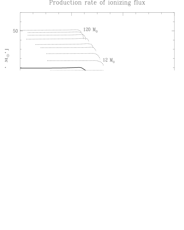
Figure 4: The boldface solid line shows the number of ionizing photons emitted per second per solar mass (without the factors $f_{\rm esc}$ and $f_{\rm star}$, see § 2.3) for the composite emissivity shown in Figure 3 and a Scalo IMF. The boldface dashed line shows the rate for a tilted Scalo IMF, where most of the stars have low masses. The dotted lines show the separate contributions from stars with masses (top to bottom) 120, 85, 60, 40, 25, 20, 15, 12, 9, 7, 5, 4, 3, 2.5, 2, 1.7, 1.5, and 1.25 $M_{\odot}$, in units of photons/sec.

Figure 4 shows the expected evolution in the production rate of ionizing photons for stars with various masses between 1 and 120$M_{\odot}$ (dotted curves) and for the composite flux of a Scalo IMF (solid curve). The ionizing flux starts to decline roughly two million years after the starburst due to the limited lifetime of stars on the main sequence. The total number of ionizing photons which are released per proton processed through a star is $\sim 1100$, about two order of magnitudes lower than the corresponding value for a single O star. The dashed line shows the production rate of ionizing photons when the standard IMF is tilted by a power–law index of $\beta$=1.69 in the direction of introducing more low mass stars; this choice of $\beta$ is motivated by the possibility that the halos of galaxies are composed of Massive Compact Halo Objects (MACHOs). The lack of massive stars in the tilted IMF reduces significantly the number of ionizing photons to a total value of 0.66 ionizing photons per baryon processed through a star.

We assume that fragmentation converts a constant fraction of the gas into stars at every point inside the cloud. However, not all of the ionizing photons which are emitted by these stars, escape the cloud and ionize the IGM. The escape probability $f_{\rm esc}$ depends on the density profiles of both the gas and the stars inside the cloud. For both components, we adopt a radial density profile that varies as $\propto 1/r^{2}$ and is truncated at some outer radius, where the density jumps by a factor of $\sim 50$ from its background value. This profile is in good agreement with the numerical results described in HTL96, and is slightly shallower than the dark matter profile ($\propto 1/r^{2.25}$) predicted by self–similar solutions (Bertschinger 1985). Under the assumption of a constant $f_{\rm star}$ throughout the cloud, we calculate the equilibrium ionization profile both inside and outside the cloud by solving the equations of radiative transfer and ionization equilibrium,

$$F_{\nu}(r)=\frac{1}{r^{2}}\int_{0}^{r}r^{\prime 2}e^{-\tau_{\nu}(r,r^{\prime})}j_{\nu}(r^{\prime})dr^{\prime},$$ (2)

$$\tau_{\nu}(r,r^{\prime})=\sigma_{\nu}\left[N_{\rm H}(r)-N_{\rm H}(r^{\prime})\right],$$ (3)

$$\alpha_{\rm B}(T)n_{\rm e}^{2}=n_{\rm H}\int_{\nu_{\rm H}}^{\infty}\frac{4\pi\sigma_{\nu}F_{\nu}}{h_{\rm P}\nu}d\nu,$$ (4)

where $j_{\nu}$=$\epsilon_{\nu}f_{\rm star}\rho_{\rm b}(r)/(4\pi)$ is the monochromatic emission coefficient in units of ${\rm erg}$ ${\rm cm^{-3}}$ ${\rm s^{-1}}$ ${\rm ster^{-1}}$ ${\rm Hz^{-1}}$; $F_{\nu}$ is the flux in units of ${\rm cm^{-2}~{}s^{-1}}$; $\tau_{\nu}(r,r^{\prime})$ is the optical depth between radii $r$ and $r^{\prime}$; $\sigma_{\nu}$ is the ionization cross–section of hydrogen in units of ${\rm cm^{2}}$; $N_{\rm H}(r)$=$\int_{o}^{r}n_{\rm H}(r)dr$ is the column density of neutral hydrogen between the center and a radius $r$; $\alpha_{\rm B}(T)$=$2.6\times 10^{-13}~{}{\rm cm^{3}~{}s^{-1}}$ is the case B recombination coefficient at $T\approx 10^{4}$K; $n_{\rm e}$ and $n_{\rm H}$ are the number densities of electrons and neutral atoms in ${\rm cm^{-3}}$; $\rho_{\rm b}(r)$ is the mass density profile of the gas; $\nu_{\rm H}$ is the ionization threshold of hydrogen, and $h_{\rm P}$ is Planck’s constant.

Figure 5 shows an example of the resulting ionization profile for an object with a baryonic mass of $10^{6}{M_{\odot}}$ at $z=50$. The size of this object is $\sim 150$ pc, and the vertical dashed line at $\sim 2.5$ kpc shows the size that the associated Strömgren sphere would have had if the recombinations inside the object were ignored and only the recombinations in the background gas were taken into account. The recombinations inside the object reduce the size of the Strömgren sphere to $\sim 0.8$kpc, from where we infer that only a fraction $f_{\rm esc}\approx(0.8/2.5)^{3}=3.3\%$ of the ionizing photons escaped from the object.

We have computed similar equilibrium ionization profiles for objects of different masses and redshifts, and in each case we obtained the escape fraction $f_{\rm esc}$. The results are shown in Figure 6 for objects with masses between $10^{4}M_{\odot}$ (top curve) and $10^{9}M_{\odot}$ (bottom curve). This figure demonstrates that the escape fraction varies only slightly with mass but depends strongly on redshift. At redshifts below $z=10$ the escape fraction is close to unity; at higher redshifts one can derive a useful fitting formula, accurate to within $\sim$ 10%,

$$\log f_{\rm esc}=\left\{\matrix{1.92\{\exp[-(z-10)^{2}/1510]-1\}\hfill&({\rm for}~{}z>10)\hfill\cr 0\hfill&({\rm for}~{}z\leq 10)\hfill.\cr}\right.$$ (5)

Although the escape fraction of the ionizing photons is a crucial ingredient in all of our reionization models, little is known about its value in nearby star forming regions. For reference, it is possible to compare our estimates with the value of 14% obtained by Dove & Shull (1994) in their theoretical modeling of HII regions around OB associations inside the exponential disk of the Milky Way galaxy (short dashed line in Fig. 6). Another possible comparison is with the value of 3% reported by Leitherer et al. (1995) from observations of four nearby starburst galaxies (long dashed line). On the one hand, our approach overestimes the escape fraction because it ignores small scale clumpiness of the gas. On the other hand, it underestimates the escape fraction, because the system might lose its gas due to winds driven by supernova explosions or photoionization heating. The dependence of our results on changes in the adopted values of the escape probability is discussed in §4.

2.3 Propagation of the Ionization Fronts

The propagation of ionization fronts in an expanding medium was considered by Shapiro & Giroux (1987) in the context of reionization of the universe by quasars. The temporal evolution of the radius of the ionization front $r_{\rm i}$ in physical (i.e. not comoving) coordinates is determined by the equation

$$n_{\rm H}\left(\frac{dr_{\rm i}}{dt}-H(t)r_{\rm i}\right)=\frac{1}{4\pi r_{\rm i}^{2}}\left(\frac{dN_{\gamma}}{dt}(t)-\frac{4}{3}\pi r_{\rm i}^{3}\alpha_{\rm B}n_{\rm H}^{2}\right),$$ (6)

where $H(t)$ is the Hubble constant, ${dN_{\gamma}/{dt}}(t)$ is the emission rate of ionizing photons by the source, and $n_{\rm H}$ is the background number density of neutral hydrogen in the IGM. Equation (6) simply expresses the fact that during the expansion of the ionization front, the ionization rate of fresh atoms is equal to the difference between the emission rate of photons from the source and the total recombination rate in the already ionized region. In the case of a steady source ($dN_{\gamma}/dt$=const), equation (6) can be solved analytically (Shapiro & Giroux 1987) for $r_{\rm i}(t)$; with a time-dependent source, we substitute ${dN_{\gamma}}/{dt}(t)$ and obtain $r_{\rm i}(t)$ numerically. In our model,

$$\frac{dN_{\gamma}}{dt}(t)=f_{\rm esc}f_{\rm star}M_{\rm b}\int_{\nu_{\rm H}}^{\infty}d\nu\frac{\epsilon_{\nu}}{h_{\rm P}\nu},$$ (7)

where $M_{\rm b}$ is baryonic the mass of the source, $f_{\rm esc}$ is the escape fraction of photons from the source, $f_{\rm star}$ is the fraction of gas converted to stars, and $\epsilon_{\nu}$ is the composite stellar emissivity per unit mass.

It is instructive to examine the evolution of the ionization front in units of the time–dependent Strömgren radius of a steady source at the initial luminosity,

$$r_{\rm s}=\left[\frac{3}{4\pi\alpha_{\rm B}n_{\rm H}^{2}(t)}{dN_{\gamma}\over dt}(t=0)\right]^{1/3}.$$ (8)

Figure 7 illustrates the evolution of the ionization front in units of the Strömgren radius for sources that turn on at different redshifts between 10–100, and have the ionizing photon production rate shown in Figure 4. Two interesting effects are apparent:

• The ionization front reverses its direction of propagation when the flux from the source starts to decline (cf. Fig. 4). The decrease in the volume of the HII region can be substantial at high redshifts, when the recombination time in the IGM is short.

• At redshifts $z\lesssim 10^{2}$, the ionization front does not have sufficient time to expand to its full Strömgren radius, as pointed out by Shapiro and Giroux (1987). This effect is less important at high redshifts, because the recombination time in the IGM is then shorter and the Strömgren radius is therefore closer to the source.

Note that our calculation assumes that the ionization front propagates out from a virialized nonlinear object into a uniform IGM. Numerical simulations (such as described in Gnedin & Ostriker 1996) are necessary in order to explicitly incorporate the mildly nonlinear IGM clumpiness in this calculation.

2.4 Carbon Production and Star Formation Efficiency

Because we presently lack a standard theory of star formation, our models (as well as other studies, such as Fukugita & Kawasaki 1994, and Madau & Shull 1996) simply assume that a constant fraction $f_{\rm star}$ of the gas is transformed into stars. Our approach is to calibrate $f_{\rm star}$ based on the inferred carbon abundance in the IGM from Keck observations of the Ly$\alpha$ forest (Cowie et al. 1995; Tytler et al. 1995; Songaila & Cowie 1996, Cowie 1996). The low column density absorbers in the Ly$\alpha$ forest extend over large transverse scales of $\gtrsim 0.1$–$1$ Mpc (Bechtold et al. 1994; Dinshaw et al. 1994, 1995; Fang et al. 1995; Smette et al. 1995) and can be interpreted as mildly overdense regions in a photoionized IGM (Hernquist et al. 1996, Miralda-Escudé et al. 1995). We assume that the apparently universal metallicity of these systems resulted from metal enrichment by many low–mass ($\sim 10^{8-9}M_{\odot}$) star clusters inside of them. In our standard model we adopt the most conservative approach which assumes that all the metals produced by the stars are mixed efficiently with the IGM; a lower mixing efficiency would imply a higher value for $f_{\rm star}$ and an even earlier reionization epoch for the same value of IGM metallicity. The required mixing of the metal rich gas with the IGM could have resulted from supernova driven winds, since the velocity dispersion of the systems which are responsible for reionization in our models is only $\sim 10~{}{\rm km~{}s^{-1}}$. However, even if some metallicity gradients remained because of incomplete mixing, the line-of-sight integral inherent to observations of the Ly$\alpha$ forest systems tends to average over these variations and yield a roughly universal metallicity value throughout the universe.

We assume that the same population of stars that produced the heavy elements detected in the Ly$\alpha$ absorbers is responsible for the reionization of the universe. In order to fix $f_{\rm star}$, we need to specify the amount of heavy elements produced by a population of stars with the Scalo IMF. Since the Keck observations detected specifically CIV absorption lines, we focus our attention on stellar yields of ¹²C. The carbon yields of high mass stars are well established in the literature. Weaver & Woosley (1993) have calculated the yields for stars with masses between 11–40${M_{\odot}}$, and their numbers are in good agreement with the yields reported by Maeder (1992) for stars with 9–120${M_{\odot}}$. For low and intermediate mass stars with 1–8${M_{\odot}}$, the yields were tabulated by Renzini & Voli (1981), and more recently by van den Hoek & Groenwegen (1996). However, since these stars do not explode as supernovae, there is a significant uncertainty about the amount of carbon that actually gets ejected from these stars to the surrounding medium (e.g. through thermal pulsations or winds). This uncertainty is particularly large for stars which are more massive than $\sim 3{M_{\odot}}$, as these stars are known to undergo some amount of “hot bottom burning”, i.e. burning of carbon into nitrogen at the base of their convective envelopes. The actual amount of hot bottom burning depends sensitively on the convective mixing length, and is highly uncertain.

Figure 8 shows the carbon yields as a function of stellar mass. The large range of yields allowed for 3–8${M_{\odot}}$ stars is due to the unknown efficiency of hot bottom burning. Additional uncertainty in the total carbon yield results from the unknown stellar IMF; Figure 9 shows the maximum allowed carbon yields folded in with a Scalo (1986), Miller–Scalo (1979), and tilted Scalo IMFs. In our standard model we adopt the first choice. The sensitivity of our results to variations in these uncertain parameters will be examined in § 4.

Figures 8 and 9 show that most of the carbon is produced by 3–6${M_{\odot}}$ stars, and therefore the total amount of carbon output by all stars is subject to the uncertainties about hot bottom burning. In order to get an average carbon enrichment equivalent to 1%$Z_{\odot}$, as measured in the Ly$\alpha$ forest, it is necessary that a nominal 2.8% of all the baryons be converted into stars with a Scalo IMF (or a fraction 1.2% for a Miller–Scalo IMF). The corresponding required value of the star–formation efficiency for the Scalo IMF is $f_{\rm star}=13\%$. Here, a factor of $\sim 2.3$ increase is from the average time required to produce carbon inside the stars; i.e. only a fraction 1/2.3 of the total stellar carbon is produced by $z=3$; another factor of 2 increase is from the value of the collapsed fraction, $F_{\rm coll}=50\%$ at $z=3$. Note that $f_{\rm star}$ must be increased further if any significant amount of hot bottom burning occurs in stars with 3–8${M_{\odot}}$.

Finally, it is interesting to note that most of the carbon enrichment is due to stars with 3–6${M_{\odot}}$, while most of the ionizing photons are produced by stars with 10–12${M_{\odot}}$. Because of this fact, the carbon enrichment is delayed considerably relative to the photon production; 90% of ionizing photons are emitted already within $\sim 5\times 10^{7}$ years following the starburst, while it takes $\sim 5\times 10^{8}$ years to eject 90% of the total carbon output.

3 Consequences of the Model

Next, we use the model described in the previous section to calculate the redshift evolution of various integral quantities, i.e. the fraction of baryons contained in collapsed objects, the average metallicity of the IGM, the volume filling factor of ionized regions, the microlensing probability, and the optical depth to electron scattering which translates to a damping factor for the cosmic microwave background (CMB) anisotropies. Below we discuss each of these quantities separately.

The Collapsed Fraction

The fraction of baryons contained in collapsed objects is given in equation (1). In our model, a fixed universal fraction $f_{\rm star}$ of this material is converted into stars. However, as argued in §2, fragmentation of the collapsed clouds into stars is initially inhibited by the photo–dissociation of ${\rm H_{2}}$ (cf. HRL97). Shortly after the very first ionizing sources turn on, ${\rm H_{2}}$ cooling is suppressed even in dense environments. Star formation resumes when clouds with a virial temperature $\gtrsim 10^{4}$K, or a total mass $\gtrsim 10^{8}{M_{\odot}}[(1+z)/10]^{-3/2}$ collapse, inside which atomic line cooling becomes efficient and triggers fragmentation. We incorporate this pause in the star-formation history into our model by setting $f_{\rm star}=0$ in equation (1) for clouds with masses below $10^{8}{M_{\odot}}[(1+z)/10]^{-3/2}$. Note, however, that star formation is suppressed by a factor of $\sim[1-F_{\rm HII}(z)]$ even in the absence of ${\rm H_{2}}$-feedback; the collapse of clouds in a hot ($\sim 10^{4}~{}{\rm K}$) photoionized gas is delayed until dark-matter potential wells with sufficient depth form (Couchman & Rees 1986). We therefore multiply $f_{\rm star}$ by $[1-F_{\rm HII}(z)]$ in one of the variants on our standard model where ${\rm H_{2}}$-feedback is ignored.

Metallicity

We obtain the average metallicity of the IGM from the carbon yields as described in § 2.4. Our standard model assumes that each star deposits all of its carbon yield in the background gas at the end of its life on the main sequence, and that the metal enriched gas is fully mixed with the IGM. We define $f_{\rm carb}(\Delta t)$ to be the fraction of the total carbon yield which gets deposited after a time $\Delta t$ following the starburst. As a result of this deposition, the IGM obtains a carbon metallicity

$$Z(z)=0.01Z_{\odot}\times\left(\frac{f_{\rm star}}{0.028}\right)\int_{\infty}^{z}dz^{\prime}\frac{dF_{\rm coll}}{dz}(z^{\prime})f_{\rm carb}\left[t(z)-t(z^{\prime})\right].$$ (9)

The value $f_{\rm star}=0.028$ would result in the required metallicity $0.01Z_{\odot}$ if the collapsed fraction $F_{\rm coll}$ was unity and there was no time–delay in the carbon prodcution (assuming the maximum possible carbon yields with a Scalo IMF, cf. § 2.4). $Z(z)$ is proportional to $F_{\rm coll}(z)$ only at low redshifts when the finite time needed to deposit the carbon yields is much shorter than the Hubble time.

HII Filling Factor

Our model can be used to determine the fraction of the volume of the universe in which hydrogen is ionized as a function of redshift. We define $r_{\rm i}(z_{\rm on},z,M)$ to be the time dependent radius of the spherical ionization front around a source of mass $M$ which turns on at a redshift $z_{\rm on}$. Equation (6) can then be used to determine $r_{\rm i}(z_{\rm on},z,M)$ for a range of $z$ and $M$ values. Since the escape fraction of ionizing photons $f_{\rm esc}$ is, to leading order, independent of the mass of the system, the volume ionized by a given system scales linearly with its mass, namely $V_{\rm HII}(z_{\rm on},z,M)=(4\pi r_{\rm i}^{3}/3)=M\times{\tilde{V}}_{\rm HII}(z_{\rm on},z)$, where ${\tilde{V}}_{\rm HII}(z_{\rm on},z)$ is the ionized volume per unit mass. We can therefore evaluate the HII filling factor $F_{\rm HII}(z)$ from the collapsed gas fraction

$$F_{\rm HII}(z)=\rho_{\rm b}(z)\int_{\infty}^{z}dz^{\prime}\frac{dF_{\rm coll}}{dz}(z^{\prime}){\tilde{V}}_{\rm HII}(z^{\prime},z),$$ (10)

where $\rho_{\rm b}=\Omega_{\rm b}\rho_{\rm crit}$ is the average baryonic density and $\rho_{\rm crit}$ is the critical density of the universe. Note that this result depends only the total fraction of baryons in nonlinear objects and not on the merger history of these objects.

Microlensing Optical Depth

The probability for having a microlensing event along the line-of-sight to a point source located at a redshift $z_{\rm S}$ in an $\Omega_{0}=1$ universe, is given by,

$$\tau_{\rm lens}(z_{\rm S})=\frac{\Omega_{\rm b}\rho_{\rm crit}c}{H_{0}}\int_{o}^{z_{\rm S}}dz_{\rm L}\sqrt{1+z_{\rm L}}f_{\rm star}F_{\rm coll}(z_{\rm L})\sigma_{\rm lens}(z_{\rm L}),$$ (11)

where $c$ is the speed of light, and the cross–section per unit mass associated with the Einstein ring of the lenses has the form (Gould 1995; Turner, Ostriker & Gott 1984):

$$\sigma_{\rm lens}(z_{\rm L})=\frac{4\pi G}{c^{2}}\frac{x_{\rm L}(\lambda_{\rm S}-\lambda_{\rm L})\lambda_{\rm L}}{\lambda_{\rm S}}.$$ (12)

Here the subscripts L and S refer to the lens and the source, $x\equiv(1+z)$, and

$$\lambda\equiv\frac{2}{5}\frac{c}{H_{0}}\left({1-x^{-5/2}}\right).$$ (13)

We implicitly assume that the intergalactic star clusters are intrinsically optically thin to microlensing.

Optical Depth to Electron Scattering

The optical depth to electron scattering out to a redshift $z$ in an $\Omega_{0}=1$ universe, is given by,

$$\tau_{\rm es}(z)=0.053\Omega_{\rm b}h\int_{0}^{z}dz^{\prime}\sqrt{1+z^{\prime}}\left[1-f_{\rm star}F_{\rm coll}(z^{\prime})\right]F_{\rm HII}(z^{\prime}),$$ (14)

where we used the fact that the average ionization fraction is equal to the HII filling factor. We have implicitly assumed that the fraction of singly ionized helium is $F_{\rm HII}$, and that no helium is ionized twice due to the sharp drop in our template spectrum at the HeII edge (cf. Fig. 3).

CMB Anisotropy Damping

The CMB anisotropies are damped on scales smaller than the apparent angular size of the horizon at the reionization epoch ($\sim 10^{\circ}$), due to scattering off free electrons. Hu & White (1996) provide a fitting formula for the damping factor of the CMB power–spectrum, $R_{l}^{2}$, as a function of the index $l$ in the spherical harmonic decomposition of the microwave sky [the angular scale corresponding to a given $l$–mode is $\sim 1^{\circ}\times(l/200)^{-1}$]. The damping factor is uniquely related to the scattering optical depth as a function of redshift, $\tau_{\rm es}(z)$, which is given by equation (14) (see also Kamionkowski et al. 1994).

Table 1: The assumed parameter values in our standard model and its variants.

Parameter	Standard Model	Range Considered
$\sigma_{8h^{-1}}$	0.67	0.67–1.0
$n$	1.0	0.8–1.0
$\Omega_{\rm b}$	0.05	0.01–0.1
$f_{\rm star}$	13%	1%–40%
$f_{\rm esc}$	$f_{\rm esc}(z)$	3%–100%
IMF tilt ($\beta$)	0	0–1.69
${\rm H_{2}}$ feedback	yes	yes/no

4 Results and Discussion

Figures 10–15 show results from our reionization models. We define our “standard model” by the set of parameters summarized in Table 1, and analyze the sensitivity of the results to separate changes in the values of each parameter. Our choice for the cosmological parameters follows standard CDM with a scale–invariant power spectrum, and the likely nucleosynthesis value for the baryon density (Copi, Schramm & Turner 1995), namely $n$=1, $h$=0.5, $\Omega=1$, $\Omega_{\rm b}$=0.05. The COBE normalization of this power spectrum implies $\sigma_{8h^{-1}}$=1.22, which predicts too much power on small scales and is ruled out by observations (Bunn & White 1996). We therefore use as our standard value $\sigma_{8h^{-1}}$=0.67 (an upper limit based on cluster abundance, see White, Efstathiou, & Frenk 1993; Bond & Myers 1996; Viana & Liddle 1996). It is important to note that our results depend primarily on the behavior of the power spectrum on small scales and have little sensitivity to its characteristics on large scales, where direct constraints from galaxy surveys and microwave anisotropy experiments apply. In our standard model, we adopt a Scalo stellar IMF with the maximum carbon output (i.e. the minimum amount of ionizing photons for a given metallicity), and assume the existence of a negative feedback on star–formation due to photodissociation of ${\rm H_{2}}$. The standard star formation efficiency $f_{\rm star}$ is chosen to be 13%, so as to yield a metallicity of $0.01Z_{\odot}$ at a redshift $z=3$, where the collapsed fraction is $F_{\rm coll}\approx 50\%$ (cf. §2.4). The standard escape fraction $f_{\rm esc}$ is explicitly calculated at each redshift as described in § 2.2 and shown in Figure 6.

The results from our standard model are described by the solid lines in Figures 10–15. In this model, reionization occurs at $z=18$, with a corresponding scattering optical depth of $\tau_{\rm es}=0.07$. This leads to a $\sim 14\%$ reduction in the power of CMB anisotropies on angular scales $\lesssim 10^{\circ}$. The microlensing optical depth is small, $\tau_{\rm lens}\lesssim 2\times 10^{-3}$, even at high redshifts. Figure 10 also shows results for a higher normalization ($\sigma_{8h^{-1}}$=1.0) and a tilt ($n$=0.8) of the CDM power spectrum. With these variations, the reionization redshift changes to $z$=22 and $z$=13, and the scattering optical depth changes to $\tau_{\rm es}=0.11$ and $\tau_{\rm es}=0.04$, respectively. The low level of these changes demonstrates that our results are robust for popular variants of the CDM power spectrum.

Next, we consider the dependence of the results on the baryon density. Figure 11 shows the cases of $\Omega_{\rm b}$=0.01 and 0.1. The microlensing optical depth is simply proportional to $\Omega_{\rm b}$, while the electron scattering optical depth for these cases is $\tau_{\rm es}=0.02$ and $\tau_{\rm es}=0.13$, respectively. The deviation from the exact proportionality $\tau_{\rm es}\propto\Omega_{\rm b}$ is due to the increased recombination rate in a high baryon density universe, which slightly decreases the reionization redshift.

Figure 12 illustrates the significance of changing the star formation efficiency $f_{\rm star}$. Although $f_{\rm star}$ is directly constrained by the observed IGM metallicity, there are two reasons to consider variations in this parameter. First, there is approximately an order of magnitude uncertainty in the observed value of the CIV/H ratio; this makes the metallicity and therefore $f_{\rm star}$ uncertain by the same factor. Second, if hot bottom burning is efficient, it could eliminate the carbon yields from 3–8${M_{\odot}}$ stars, and increase $f_{\rm star}$ by up to a factor of 4. We therefore examine the cases $f_{\rm star}$=1% and $f_{\rm star}$=40%.

For $f_{\rm star}$=40% the reionization redshift is increased to $z$=24, but (i) the reionization in this case is more sudden; and (ii) a substantial fraction of the electrons are locked up in stars and do not contribute to $\tau_{\rm es}$ (the gas fraction is reduced by the factor $[1-f_{\rm star}F_{\rm coll}]$, cf. eq. [14]). These effects counteract the increase in the reionization redshift, and yield an optical depth, $\tau_{\rm es}=0.09$, which is only 15% higher than with $f_{\rm star}$=13%. On the other hand, $f_{\rm star}$=1% gives $\tau_{\rm es}$=0.05, again not too different from $\tau_{\rm es}$=0.07. Hence, Figure 12 demonstrates that the scattering optical depth is fairly insensitive to large variations in the carbon output.

Figure 13 demonstrates the effect of varying the IMF. Although the stellar IMF at high redshift is unknown, it is often claimed that due to the absence of metals and the lack of initial substructure, it favored massive stars (e.g. Carr, Bond, & Arnett 1984). For this reason, we show in Figure 13 the results for the Miller–Scalo IMF (dotted lines), which is biased towards massive stars relative to the standard Scalo IMF (solid lines). Note that the bias towards massive stars increases both the carbon yield and the UV photon production per solar mass. Therefore, a smaller number of stars are necessary to provide the observed metallicity ($f_{\rm star}=5$%), but these stars produce more ionizing photons. As the figure shows, the two effects almost cancel each other, and reionization with the Miller–Scalo IMF occurs at $z=14$, close to the redshift with the Scalo IMF.

On the other hand, the possibility still exists that the high–redshift IMF is biased in the opposite sense, i.e. towards low–mass stars. Indeed, in order to identify the early stars with MACHOs which contribute significantly to the mass of galaxy halos, a substantial fraction of the baryons must be converted into stars, and most of these stars must have low masses, $\;\hbox to0.0pt{\lower 2.5pt\hbox{$\sim$}\hss}\raise 1.5pt\hbox{$<$}\;0.5{\rm M_{\odot}}$ (Flynn et al. 1996; Alcock et al. 1996). We therefore assume $f_{\rm star}=90\%$. The tilt necessary to increase $f_{\rm star}$ from 13% to 90% while keeping the metallicity fixed, must decrease the total carbon yield per unit mass by a factor of 60. This is achieved by adding a constant $\beta=1.69$ to the power–law index in all segments of the Scalo IMF. This tilt decreases the average stellar mass from $0.5{\rm M_{\odot}}$ to $0.25{\rm M_{\odot}}$ (cf. Fig. 9). The dashed lines in figure 13 shows that with this tilt, stellar reionization is delayed substantially down to $z\sim 1$ (at which point quasars, which are ignored in this work, dominate the ionizing background). This delay is caused by the lack of ionizing photons from massive stars and is therefore a robust conclusion; combining a tilt with $f_{\rm esc}=100\%$ only increases the reionization redshift up to $z\sim 2$.

According to Figure 13, a tilted IMF increases the optical depth to microlensing substantially up to values as high as 3% at $z$=5 or 4% at $z\;\hbox to0.0pt{\lower 2.5pt\hbox{$\sim$}\hss}\raise 1.5pt\hbox{$>$}\;30$. Such microlensing probabilities could leave detectable signatures in large samples of high redshift quasars. Microlensing could either be detected through measurements of the variability of quasars or the systematic changes in the equivalent width of their emission lines. The variability signature requires an impractically long observing period (of order tens of years for solar mass lenses), and is difficult to separate from an intrinsic variability signal. The equivalent–width change results from the fact that a stellar lens could magnify the quasar continuum source, which is typically smaller than its Einstein radius $\sim 10^{16}(M_{\star}/0.1M_{\odot})^{1/2}~{}{\rm cm}$, but would not magnify the broad line region which is much more extended (see Dalcanton et al. 1994, and references therein).

Figure 14 shows the results with and without the ${\rm H_{2}}$-photodissociation feedback on star-formation. Even though the collapsed baryonic fraction is much higher without this feedback, in both cases reionization occurs at about the same redshift, $z\approx 20$. The similarity in the reionization redshifts results from the fact that when the HII filling factor approaches unity, star formation is suppressed both with and without the ${\rm H_{2}}$ feedback (cf. § 3). The total optical depth to electron scattering without the ${\rm H_{2}}$–feedback is increased to $\tau_{\rm es}=0.11$; most of the difference from the case with the ${\rm H_{2}}$–feedback is introduced when the universe is only partially ionized.

Figure 15 illustrates the sensitivity of the results to the escape fraction. We show results for either the low value of $f_{\rm esc}$=3% observed in nearby starburst galaxies (Leitherer et al. 1996), or the hypothetical high value of 100%. The motivation for considering $f_{\rm esc}$=100% is the theoretical possibility that the obscuring gas could be expelled from the star forming clouds by photoionization heating or supernova–driven winds. Such an expulsion of the gas would then quench further star-formation in these systems (Lin & Murray 1992); this mechanism could explain why the star formation efficiency is limited to 13%. In this work, however, we normalize the star formation efficiency based on the metallicity of the Ly$\alpha$ forest, without attempting to explain its origin. In the case of a low escape fraction, the resulting optical depth for electron scattering is decreased to $\tau_{\rm es}$=0.05, with reionization still occurring at $z$=11. In the case of a high escape fraction, the optical depth and reionization redshifts are increased by a negligible fraction.

In addition to the above indirect signatures of reionization, it is interesting to examine the possibility of a direct imaging of the reionization sources. Although any such imaging is beyond the sensitivities of current instruments, the Next Generation Space Telescope (NGST) will achieve a suitable sensitivity for that purpose, $\sim 1$ nJy in the wavelength range 1–3.5$\mu$m (Mather & Stockman 1996; see also http://ngst.gsfc.nasa.gov). In Figure 16 we show the predicted number of objects that NGST would detect as a function of observed flux, assuming a sudden reionization at the redshift $z_{\rm ion}=18$. The number counts are normalized to the field of view of the Space Infrared Telescope Facility (SIRTF) $5^{\prime}\times 5^{\prime}$, which is scheduled for launch long before NGST (the planned field-of-view of NGST is similar, $4^{\prime}\times 4^{\prime}$). The abundance and emissivity of each source was calculated according to our standard model as described in § 2.1-2.2. We have averaged the flux from each source over the range of 1–3.5$\mu$m and truncated the spectra of all objects at emission frequencies above Ly$\alpha$ before reionization occurs, since the optical depth of HI at these frequencies is exceedingly high prior to reionization.

Figure 16 shows the number per logarithmic flux interval of all objects at $z>5$ (top curve), and all objects at $z>10$ (bottom curve). The number of detectable sources is high. With its expected sensitivity, NGST will be able to probe about $10^{4}$ objects at $z>5$. The average separation between these compact sources would be of order 2.4˝, well above the angular resolution of 0.06˝, planned for NGST.

Another detectable signature of a reionized IGM results from its Bremsstrahlung emission. In an $\Omega=1$ universe, the surface brightness observed today is given by (Loeb 1996)

$$J_{\rm ff}(\nu)=\frac{c}{H_{0}}\int_{\infty}^{0}\frac{j_{\rm ff}[(1+z)\nu]dz}{(1+z)^{11/2}},$$ (15)

where the free–free emissivity $j_{\rm ff}$ at very low frequencies is independent of frequency (we ignore the logarithmic frequency–dependence of the Gaunt factor), and is given by (Rybicki & Lightman 1979)

$$j_{\rm ff}(\nu)=3.1\times 10^{-40}\frac{\langle n_{\rm e}^{2}\rangle}{(T/10^{4}{\rm K})^{0.5}}~{}~{}~{}{\rm{erg~{}cm^{-3}~{}s^{-1}~{}Hz^{-1}~{}sr^{-1}}}.$$ (16)

The value of $\langle n_{\rm e}^{2}\rangle$ at each redshift is a sum of the contributions from the ionized regions of the smooth IGM and the star–forming clouds themselves,

$$\langle n_{\rm e}^{2}\rangle=F_{\rm HII}(1-F_{\rm coll})\langle n_{\rm e}^{2}\rangle_{\rm IGM}+\int_{\infty}^{z}dz^{\prime}\frac{dF_{\rm coll}}{dz}(z^{\prime})\langle n_{\rm e}^{2}\rangle_{{}_{\star}}[t(z)-t(z^{\prime})].$$ (17)

In our standard model, the average value of $n_{\rm e}^{2}$ within an ionized region of the smooth IGM is simply given by $\langle n_{\rm e}^{2}\rangle_{\rm IGM}=[1.15\times 10^{-7}(1+z)^{3}]^{2}~{}~{}{\rm cm}^{-6}$. The average of $n_{\rm e}^{2}$ within each star forming cloud can be obtained by noticing that the recombination rate in each cloud is simply $(1-f_{\rm esc})$ times the production rate of ionizing photons, i.e.

$$\langle n_{\rm e}^{2}\rangle_{{}_{\star}}[\Delta t]\equiv\frac{1}{\frac{4}{3}\pi R^{3}}\int_{0}^{R}4\pi r^{2}drn_{\rm e}^{2}(r)=\frac{1}{\alpha_{\rm B}}\frac{1}{\frac{4}{3}\pi R^{3}}\left({1-f_{\rm esc}\over f_{\rm esc}}\right)\frac{dN_{\gamma}}{dt}[\Delta t].$$ (18)

This result for the clumpiness factor is independent of the cloud mass and is only a function of the time lag since the starburst occurred, $\Delta t$. The escape fraction $f_{\rm esc}$ in this expression was derived in § 2.2 (cf. Fig. 6), and the time–dependent production rate of ionizing photons $dN_{\gamma}/dt$ was calculated in § 2.3 (cf. eq. 7 and Fig. 4).

The resulting brightness temperature, $T_{\rm b}\equiv(c^{2}J_{\rm ff}/2k\nu^{2})$, of the microwave sky due to Bremsstrahlung emission by star–forming clouds at $z>10$ and the smooth IGM, is shown in Figure 17 for the frequency range $\nu=1$–$100$ GHz. The existence of Bremsstrahlung emission from star forming regions relies on their ability to retain their gas during the lifetime of their stellar population, and is therefore uncertain. Reprocessing of starlight by dust (Wright 1981, Wright et al. 1994) might add to this emission component and will be considered elsewhere (Loeb & Haiman 1997). For comparison, the long–dashed curve shows the unavoidable Bremsstrahlung signal from the Ly$\alpha$ forest clouds (with HI column densities $\lesssim 10^{17}~{}{\rm cm^{-2}}$) at $0\lesssim z\lesssim 5$, for a UV background flux of $10^{-21}~{}{\rm erg~{}cm^{-2}s^{-1}Hz^{-1}sr^{-1}}$ at the Lyman–limit (Loeb 1996). The calculation of the Ly$\alpha$ forest contribution avoids any uncertainties about the clumpiness of the IGM, because at photoionization equilibrium the line-of-sight integral of $n_{e}^{2}$ is proportional to the observed column density of neutral hydrogen. The above signals are compared to the expected sensitivity of the proposed Diffuse Microwave Emission Survey (DIMES) experiment (dashed curve, from Kogut 1996; see also http://ceylon.gsfc.nasa.gov/DIMES). The (uncertain) contribution from the star–forming clouds is comparable to the galactic free-free emission and can easily be detected by the DIMES experiment. Extreme variants of our standard model (e.g., with a larger $\Omega_{b}$ or a lower $f_{\rm esc}$) which enhance $J_{\rm ff}$ by more than an order of magnitude, might already be ruled–out by the existing COBE limits on the spectral distortion of the CMB (Mather et al. 1994; Wright et al. 1994). The unavoidable contribution of Ly$\alpha$ clouds at $z\lesssim 5$ (Loeb 1996) is detectable with the future DIMES experiment, but the emission from the smooth IGM at $z\gtrsim 10$ is just below the sensitivity of this instrument in our standard model.

5 Conclusions

For a large range of CDM models with a Scalo IMF, the universe is reionized by a redshift $\gtrsim 10$. The optical depth to electron scattering due to reionization is in the range $\sim 0.05$–$0.15$. The resulting damping amplitude of $\sim 10$–$20\%$ for microwave anisotropies on angular scales $\lesssim 10^{\circ}$, will be detectable with future satellite experiments such as MAP or PLANCK. These experiments might be able to isolate a damping amplitude of several percent if they measure the microwave polarization (Zaldarriaga 1996).

If the stellar IMF is strongly tilted relative to the local Scalo IMF so that most of the baryons are transformed into low mass stars, then stellar reionization is suppressed due to the absence of massive stars which ordinarily dominate the ionizing flux (cf. Fig. 4). In this case, however, the existence of primordial stars might be inferred from the measurable microlensing event rate that they produce in the halo of the Milky Way (Alcock et al. 1996; Flynn, Gould & Bahcall 1996) or along the lines of sight to distant quasars (Gould 1995; Dalcanton et al. 1994).

Aside from the above mentioned sensitivity to a drastic variation in the IMF, much of the qualitative results summarized in Figures 10–15 appear robust to changes in other model parameters. This robustness results from a number of reasons. The collapsed fraction depends exponentially on redshift in the rare tail of the Gaussian random field of density fluctuations–from where the first objects are drawn. The inverse dependence of the collapse redshift, and hence the scattering optical depth $\tau_{\rm es}$, on the power spectrum is therefore only logarithmic. The linear scaling of $\tau_{\rm es}$ with $\Omega_{\rm b}$ is somewhat moderated by the dependence of the recombination rate on $\Omega_{\rm b}^{2}$. The reionization redshift is not sensitive to variations in the star formation efficiency $f_{\rm star}$ or the escape fraction $f_{\rm esc}$ , because of the strong dependence of the recombination rate on redshift ($\propto[1+z]^{6}$). Finally, the suppression of star–formation due to the H₂ feedback is significant compared to the suppression due to photo–ionization heating only as long as the filling factor of ionized bubbles is still small; once the ionized bubbles start to overlap, the H₂ feedback becomes unimportant.

We have calibrated the metal production in our models based on the carbon abundance detected in the Ly$\alpha$ forest at $z\sim 3$ (Cowie et al. 1995; Tytler et al. 1995; Songaila & Cowie 1996, Cowie 1996). If the metallicity of the Ly$\alpha$ forest, as inferred from the carbon/hydrogen ratio, is indeed universal and due to a single generation of stars, then the star formation efficiency for a Scalo IMF is higher than $4\%$, or else “hot bottom burning” (which destroys carbon in stellar envelopes) is entirely inefficient. This conclusion is independent of the details of the rest of our modeling. Future detection of other metal absorption lines in the Ly$\alpha$ forest would allow to discriminate among these possibilities.

Much of the uncertainty in our reionization models results from the lack of a standard theory for star formation. Existing theoretical work on star formation has been mainly guided by observations and therefore focused, by and large, on the complex environments of the interstellar medium of our galaxy. The conditions in the early universe are much better defined than those in the local interstellar medium, since the composition of the gas and hence its chemistry and cooling function are simple and well known, the power spectrum of initial density fluctuations is prescribed in specific cosmological models, and magnetic fields are probably absent before stars form. From a theoretical standpoint, the early universe offers a simpler environment for understanding star formation. The interplay between theory and observations of the reionization epoch might therefore add insight to the physics of star formation, especially if the star clusters at high redshifts are directly imaged. Our estimates, illustrated in Figure 16, imply that deep infrared observations with the Next Generation Space Telescope might be able to probe $\gtrsim 10^{3}$ bright star clusters at $z\sim 5$–$10$. The cumulative Bremsstrahlung emission from these clusters (cf. Figure 17) could potentially be detected by future instruments such as the Diffuse Microwave Emission Survey (Kogut 1996).

We thank George Field, Peter Höflich, Wayne Hu, Rohan Mahadevan, Martin Rees, Dimitar Sasselov, David Spergel, and Martin White for stimulating discussions and useful comments. AL acknowledges support from the NASA ATP grant NAG5-3085.

REFERENCES

Alcock, C., et al. 1996, preprint astro-ph/9606165

Arons, J., & Wingert, D. W. 1972, ApJ, 177, 1

Bardeen, J.M., Bond, J.R., Kaiser, N., & Szalay, A.S. 1986, ApJ, 304, 15 (BBKS)

Bechtold, J., Crotts, A. P. S., Duncan, R. C., & Fang, Y. 1994, ApJ, 437, L83

Bertschinger, E. 1985, ApJS, 58, 39

Bond, J. R. 1995, in Theory and Observations of the Cosmic Microwave Background Radiation, ed. Schaeffer, R. (Elsevier: Netherlands), in press

Bond, J. R., & Efstathiou, G. 1987, MNRAS, 226, 665

Bond, J. R., & Myers, S. 1996, ApJS, 103, 63

Bunn, E. F., & White, M. 1996, preprint astro-ph/9607060

Carr, B. J., Bond, J. R., & Arnett, W. D. 1984, ApJ, 277, 445

Copi, C. J., Schramm, D. N., & Turner, M. S. 1995, Science, 267, 192

Couchman, H. M. P. & Rees, M. J. 1986, MNRAS, 221, 53

Cowie, L. 1996, in HST and the High Redshift Universe, Proc. 37th Herstmonceux conference, eds. Tanvir, N. R., Aragón-Salamanca, A., Wall, J.V. (World Scientific:Singapore), in press, (preprint astro-ph/9609158)

Cowie, L. L., Songaila, A., Kim, T.-S., & Hu, E. M. 1995 AJ, 109, 1522

Dalcanton, J. J., Canizares, C. R., Granados, A., Steidel, C. C., & Stocke, J. T. 1994, ApJ, 424, 550

Davidsen, A. F., Kriss, G. A., & Zheng, W. 1996, Nature, 380, 47

Dinshaw, N., Impey, C. D., Foltz, C. B., Weymann, R. J., & Chaffee, F. H. 1994, ApJ, 437, L87

Dinshaw, N., Foltz, C. B., Impey, C. D., Weymann, R. J., & Morris, S. L. 1995, Nature, 373, 223 Dove, J. B., & Shull, J. M. 1994, ApJ, 430, 222

Efstathiou, G., & Bond, J. R. 1987, MNRAS, 227, 33p

Eisenstein, D.J., & Loeb, A. 1995, ApJ, 443, 11

Fang, Y., Duncan, R. C, Crotts, A. P. S., & Bechtold, J. 1995, preprint astro-ph/9510112

Flynn, C., Gould, A., & Bahcall, J. N. 1996, ApJ, 466, 55L

Fukugita, M., & Kawasaki, M. 1994, MNRAS, 269, 563

Giroux, M. L., & Shapiro, P. R. 1996, ApJS, 102, 191

Gnedin, N. Y., & Ostriker, J. P. 1996, preprint astro-ph/9612127

Gould, A. 1995, ApJ, 455, 37

Haardt, F., Madau, P. 1996, preprint astro-ph/9609057

Haiman, Z., Thoul, A., & Loeb, A. 1996, ApJ, 464, 523 (HTL96)

Haiman, Z., Rees, M. J., & Loeb, A. 1996, ApJ, 467, 522 (HRL96)

Haiman, Z., Rees, M. J., & Loeb, A. 1997, ApJ, in press (HRL97)

Hellsten, U., Davé, R., Hernquist, L., Weinberg, D., & Katz, N. 1997, preprint astro-ph/9701043

Hernquist, L., Katz, N., Weinberg, D. H., & Miralda-Escudé, J. 1996, ApJ, 457, L51

Hu, W., & White, M. 1996, “The Damping Tail of CMB Anisotropies”, preprint astro-ph/9609079

Kamionkowski, M., Spergel, D. N., & Sugiyama, N. 1994, ApJL, 426, L57

Kogut, A. 1996, preprint astro-ph/9607100

Kurucz, R. 1993, CD-ROM No. 13, ATLAS9 Stellar Atmosphere Programs

Leitherer, C., Ferguson, H. C., Heckman, T. M., & Lowenthal, J. D. 1995, ApJ, 454, L19

Lin D. C. & Murray, S. D. 1992, ApJ, 394, 523

Loeb, A. 1996, ApJ, 459, L5

Loeb, A. & Haiman, Z. 1997, in preparation

Madau, P., & Shull, J. M. 1996, ApJ, 457, 551

Mather, J. C. et al. 1994, ApJ, 420, 439

Mather, J, & Stockman, P. 1996, ST Sci Newsletter, v. 13, no. 2, p. 15

Meiksin, A., & Madau, P. 1993, 412

Miller, G. E., & Scalo, J. M. 1979, ApJS, 41, 513

Miralda-Escudé, J., & Ostriker, J. P. 1990, ApJ, 350, 1

Miralda-Escudé, J., Cen, R., Ostriker, J. P., & Rauch, M. 1995, ApJ, submitted, preprint astro-ph/9511013

Ostriker, J. P., & Gnedin, Y. N. 1996, preprint astro-ph/9608047

Padmanabhan, T. 1993, Structure Formation in the Universe (Cambridge University Press: Cambridge)

Press, W. H., & Schechter, P. L. 1974, ApJ, 181, 425

Rauch, M., Haehnelt, M. G., & Steinmetz, M. 1996, preprint astro-ph/9609083

Rees, M. J. 1996, preprint astro-ph/9608196

Renzini, A., & Voli, M. 1981, A&A, 94, 175

Rybicki, G. B., & Lightman, A. P. 1979, Radiative Processes in Astrophysics (New York: Wiley)

Scalo, J. M. 1986, Fundamentals of Cosmic Physics, vol. 11, p. 1-278

Schaller, G., Schaerer, D., Meynet, G., & Maeder, A. 1992, A&ASS, 96, 269

Scott, D., Silk, J., & White, M. 1995, Science, 268, 829

Shapiro, P. R., & Giroux, M. L. 1987, ApJ, 321, L107

Shapiro, P. R., Giroux, M. L., & Babul 1994, ApJ, 427, 25

Songaila, A., & Cowie, L. L. 1996, AJ, 112, 335

Smette, A., Robertson, J. G., Shaver, P. A., Reimers, D., Wisotzki, L., & Köhler, Th. 1995, A&A Suppl., 113, 199

Tegmark, M., Silk, J., & Blanchard, A. 1995, ApJ, 434, 395

Tegmark, M., Silk, J., Rees, M. J., Blanchard, A., Abel, T., & Palla, F. 1996, ApJ, in press, preprint astro-ph/9603007

Turner, E. L. Ostriker, J. P., & Gott, J., R., III. 1984, ApJ, 284, 1

Tytler, D. et al. 1995, in QSO Absorption Lines, ESO Astrophysics Symposia, ed. G. Meylan (Heidelberg: Springer), p.289

van den Hoek, L. B., & Groenwegen, M. A. T. 1996, preprint astro-ph/9610030

Viana, P. T. P., & Liddle, A. 1996, MNRAS, in press, preprint astro-ph/9511007

Vikhlinin, A. A. 1995, Astron. Lett., vol. 21, no. 3., p. 366

White, S. D. M., Efstathiou, G., & Frenk, C. S. 1993, MNRAS, 262, 1023

Woosley, S. E., & Weaver, T. A. 1986, ARA&A, 24, 205

Woosley, S. E., & Weaver, T. A. 1995, A&A Supp., 101, 181

Wright, E. L. 1981, ApJ, 250, 1

Wright, E. L. et al. 1994, ApJ, 420, 450

Zaldarriaga, M. 1996, preprint astro-ph/9608050

Figure 1: Collapse redshift for cold dark matter (dashed lines) and baryons (solid lines) in spheres of various masses and overdensities (the latter in units of $\sigma(M)$ for a BBKS power spectrum). The collapse of the baryons is delayed relative to the dark matter due to gas pressure. The curves were obtained by following the motion of the baryonic and dark matter shells with a spherically symmetric, Lagrangian hydrodynamics code (HTL96). The dashed lines agree with the collapse redshift for the dark matter based on the linear extrapolation of the spherical collapse model for pressureless matter, $z_{\rm coll}=\nu\sigma/1.69-1$.

Figure 2: The fraction of baryons that managed to collapse by the time the outermost shell of the dark matter halo had collapsed. The curves were obtained with the same hydrodynamics code as in Figure 1. Six different curves are shown for the six different peak heights, $0.5\sigma-3\sigma$, as in Figure 1. These curves yield an “equivalent cosmological Jeans mass” of $10^{3}{M_{\odot}}$ (cf. § 2.1).

Figure 3: Composite emissivity per solar mass for a star cluster with a Scalo IMF. Each star is assumed to evolve on the H–R diagram according to the theoretical evolutionary tracks of Schaller et al. (1992) and to emit radiation according to the spectral atlas of Kurucz (1993). The thick line shows the steady emissivity when all the stars are still on the main sequence ($\lesssim 10^{6}$ years after the starburst). The four solid lines show the emissivity at four subsequent times (from top to bottom): $t$=3, 4, 10, and 30 million years after the starburst. Frequencies corresponding to the ionizations of hydrogen and helium are marked – note the sharp drop of the emissivity at the HeII edge.

Figure 5: Example of an equilibrium ionization profile inside and around a spherically symmetric object: the fractions $x_{\rm e}=n_{\rm e}/(n_{\rm e}+n_{\rm H})$ and $x_{\rm H}=n_{\rm H}/(n_{\rm e}+n_{\rm H})$ are shown as a function of radius. We assume that the object has a baryonic mass of $10^{6}{M_{\odot}}$ and a density profile $\propto 1/r^{2}$, with a factor of 50 drop in the density at the edge of the object ($r\sim 150$pc), outside of which the density is uniform and equal to the background value at $z$=50. A fraction $f_{\rm star}=13\%$ of the baryons in the object are converted into stars with the emission spectrum shown in Figure 3. The vertical dashed line shows the radius of the Strömgren sphere when recombinations in the object are ignored; this can be used to infer the escape fraction of ionizing photons of 3.3%.

Figure 6: Escape fraction of ionizing photons from objects of different masses at various redshifts. The curves from bottom to top correspond to baryonic masses ${10^{4,5,6,7,8,9}~{}M_{\odot}}$, and are obtained from equilibrium ionization profiles similar to Figure 5. The boldface solid line shows the fitting formula $\log f_{\rm esc}=1.92(\exp[-(z-10)^{2}/1510]-1)$ for $z>10$. For comparison, the dashed line shows the theoretical estimate of the escape fraction from the disk of the Milky Way galaxy (Dove & Shull 1994), and the dotted line shows the observed value of the escape fraction in four nearby starburst galaxies (Leitherer et al. 1996).

Figure 7: Radius of the ionization front in units of the time-varying Strömgren radius (cf. eq. 8), for sources that turn on between redshifts $z$=10 and $z$=100, and have the photon production rate shown by the solid line in Figure 4. The turn-on redshifts of the 17 curves are equally spaced in log $z$.

Figure 8: Carbon yields (${\rm M_{{}^{12}C}}$ in solar masses) from stars of different masses. The large allowed range in the yields between 3–8 ${\rm M_{\rm\odot}}$ in Renzini & Voli (1981) is due to the uncertainty in the extent of hot bottom burning; $\alpha=1.5$ and 0 correspond to efficient, or no hot bottom burning, respectively.

Figure 9: Upper panel: three different initial mass functions (IMFs). The Scalo (1986) and Miller-Scalo (1979) IMFs are two different parameterizations of the locally observed stellar population, and the tilted Scalo IMF is obtained by adding a constant $\beta$=1.69 to the power law index in each segment of the Scalo IMF, while keeping the value of the IMF fixed at $4{M_{\odot}}$. All three IMFs are normalized to an integral of $1{M_{\odot}}$. Lower panel: carbon yields from stars of different masses (${\rm M_{{}^{12}C}}$, in solar masses), folded in with the three different IMFs. In all cases, most of the carbon is produced by $\sim 3$–$6{M_{\odot}}$ stars.

Figure 10: The different panels show (i) the collapsed fraction of baryons; (ii) the average metallicity of the IGM; (iii) the volume filling factor of ionized regions; (iv) the optical depth to microlensing; (v) the optical depth to electron scattering; and (vi) the net damping factor for the power–spectrum decomposition of CMB anisotropies as a function of the spherical harmonic index $l$. In this figure we examine the sensitivity of the results to changes in the normalization $\sigma_{8h^{-1}}$ or the primordial index $n$ of the CDM power–spectrum.

Figure 11: Same as Figure 10, but showing the sensitivity of the results to different values of the baryon density parameter, $\Omega_{\rm b}$.

Figure 12: Same as Figure 10, but showing the sensitivity of the results to a change in the star formation efficiency $f_{\rm star}$. If the carbon output from the stars is kept fixed, then a change in $f_{\rm star}$ translates to a proportional change in the metallicity, as shown in the upper right panel. However, the carbon yield from stars is uncertain, and thus for the other panels–an increase of $f_{\rm star}$ by some factor may also be viewed as a decrease in the carbon yield by the same factor, while keeping the IGM metallicity fixed.

Figure 13: Same as Figure 10, but showing the effect of tilting the Scalo IMF, i.e. making it steeper by adding a constant $\beta$=1.69 to the power law index in each segment. Results are also shown for a Miller–Scalo IMF which shows the opposite bias in that it contains more high mass stars than the Scalo IMF.

Figure 14: Same as Figure 10, but showing the significance of the negative feedback on star formation due to the photodissociation of ${\rm H_{2}}$.

Figure 15: Same as Figure 10, but showing the sensitivity of the results to changes in the the escape fraction of ionizing photons, $f_{\rm esc}$.

Figure 16: The number per logarithmic flux interval of high–redshift objects which could be probed by future space telescopes, in the wavelength range of 1–3.5$\mu$m. In this calculation, we assume sudden reionization at $z$=25. The vertical dashed lines show the expected sensitivities of the Space Infrared Telescope Facility (SIRTF) and the Next Generation Space Telescope (NGST).

Figure 17: Observed brightness temperature from Bremsstrahlung emission by star–forming clouds at $z>10$ and ionized regions of the smooth IGM in our standard model. The emission from the star–forming clouds exists only if the clouds retain their gas over the lifetime of their stellar population. For comparison, we show the Bremsstrahlung emission from the Ly$\alpha$ forest between $0<z<5$ for a UV background of $10^{-21}~{}{\rm erg~{}cm^{-2}s^{-1}Hz^{-1}sr^{-1}}$ at the Lyman–limit (Loeb 1996). We also show the CMB spectrum, and the proposed sensitivity of the DIMES experiment (Kogut 1996; see also http://ceylon.gsfc.nasa.gov/DIMES).