Gravitational Lensing of the X-Ray Background
by Clusters of Galaxies

Abstract

Gravitational lensing by clusters of galaxies affects the cosmic X-ray background (XRB) by altering the observed density and flux distribution of background X-ray sources. At faint detection flux thresholds, the resolved X-ray sources appear brighter and diluted, while the unresolved component of the XRB appears dimmer and more anisotropic, due to lensing. The diffuse X-ray intensity in the outer halos of clusters might be lower than the sky-averaged XRB, after the subtraction of resolved sources. Detection of the lensing signal with a wide-field X-ray telescope could probe the mass distribution of a cluster out to its virialization boundary. In particular, we show that the lensing signature imprinted on the resolved component of the XRB by the cluster A1689, should be difficult but possible to detect out to $8^{\prime}$ at the $2$–$4\sigma$ level, after $10^{6}$ seconds of observation with the forthcoming AXAF satellite. The lensing signal is fairly insensitive to the lens redshift in the range $0.1\lesssim z_{l}\lesssim 0.6$. The amplitude of the lensing signal is however sensitive to the faint end slope of the number-flux relation for unresolved X-ray sources, and can thus help constrain models of the XRB. A search for X-ray arcs or arclets could identify the fraction of all faint sources which originate from extended emission of distant galaxies. The probability for a 3$\sigma$ detection of an arclet which is stretched by a factor $\sim 3$ after a $10^{6}$ seconds observation of A1689 with AXAF, is roughly comparable to the fraction of all background X-ray sources that have an intrinsic size $\sim 1^{\prime\prime}$.

1 Introduction

The current epoch in the evolution of structure in the universe is marked by the formation of clusters of galaxies. Since clusters trace the transition between collapse and virialization, their internal structure and evolution offer a test bed for a critical examination of popular cosmological theories (e.g., Richstone, Loeb, & Turner 1992; Bahcall & Cen 1994; Cen & Ostriker 1994; Eke, Cole, & Frenk 1996).

The structure of clusters has been traditionally studied by observing their X-ray emission and the kinematics of their galaxies (e.g. Sarazin 1988; Forman & Jones 1990). More recently, deep optical imaging has allowed the use of gravitational lensing of faint galaxies to independently map the cluster mass distribution. The lensing study can be performed either in the cluster core–where the lensing signature is strong, or well outside the core–where lensing is weak (see reviews by Schneider, Ehlers, & Falco 1992; Schneider 1995; Kaiser 1995; and Narayan & Bartelmann 1996). Aside from introducing distortions to the images of extended sources, lensing changes the statistics of both the resolved (Broadhurst, Taylor, & Peacock 1995) and the unresolved (Waerbeke et al. 1996; Waerbeke & Mellier 1996) components of the extragalactic optical background. While the traditional X-ray and dynamical methods infer the cluster mass distribution by assuming spherical symmetry and virial equilibrium, the lensing techniques can measure the projected surface density distribution of the cluster free of these assumptions. The lensing methods can thus uncover deviations from spherical symmetry and equilibrium, especially in the outer regions of clusters where detection of the cluster X-ray emission is difficult.

In the current paper, we examine the imprint of lensing by galaxy clusters on the resolved and unresolved components of the cosmic X-ray background (XRB) (see also Refregier & Loeb 1996a for a brief discussion). The effect of lensing on the resolved component of the XRB typically dominates over the cluster emission at a radius of a few Mpc from the cluster center. Thus, X-ray telescopes with large fields of view ($\sim 10^{\prime}$) can probe the mass distribution of a cluster, possibly out to its virialization boundary. The information provided by the lensing method about the cluster envelope is complementary to the information obtained from the traditional X-ray emission method about the inner region of the cluster. A single deep X-ray observation can be used to study the cluster potential through both methods simultaneously.

The magnification due to lensing brings into view X-ray sources that are otherwise too faint to be resolved. With the aid of galaxy clusters as natural telescopes, one can thus reach greater sensitivity to the faint number-flux relation of extragalactic X-ray sources, and by that, unravel the origin of the X-ray background. In this work, we demonstrate, through the specific example of the cluster A1689, that lensing by individual clusters could possibly be studied with the forthcoming Advanced X-ray Astronomy Facility (AXAF) satellite, which is scheduled for launch in 1998 (Weisskopf et al. 1987; Elvis et al. 1995).

The paper is organized as follows. In §2 we approximate cluster lenses as singular isothermal spheres and model their X-ray emission phenomenologically. The cluster emission provides photon noise that masks the lensing signal in the cluster core, but declines rapidly at larger radii. We consider in detail the specific example of A1689 which we use as a test case for our study. In §3, we model the XRB by considering various extrapolations of the faint end of the number-flux relation for extragalactic X-ray sources beyond that directly observed with the ROSAT satellite. In §4, we examine the effect of lensing on these sources and on the unresolved component of the XRB. In §5, we discuss the detectability of the lensing signature for both the resolved and the unresolved components of the XRB. Finally, we summarize our conclusions in §6. Unless specified otherwise, we assume a cosmological density parameter $\Omega=1$ and a Hubble constant $H_{0}=50$ km s^-1 Mpc^-1.

2 Clusters

2.1 Lensing Model

In our lensing calculations, we model a cluster of galaxies as a Singular Isothermal Sphere (SIS) (see e.g., Schneider et al. 1992). This model provides a good first-order approximation to the projected mass distribution of known cluster lenses (Tyson & Fischer 1995; Narayan & Bartelmann 1996; Squires et al. 1996a,b).

The surface mass density of a SIS is given by

$$\Sigma(\xi)=\frac{\sigma_{v}^{2}}{2G\xi}$$ (1)

where $G$ is Newton’s constant, $\sigma_{v}$ is the line-of-sight velocity dispersion of the lens, and $\xi$ is the projected radius. This distribution has a diverging mass as $\xi\rightarrow\infty$ and should therefore be truncated at a finite value of $\xi$, of order the virialization boundary of the cluster ($\sim 5{\rm Mpc}$). The singularity of $\Sigma(\xi)$ at $\xi=0$ can be removed through the addition of a core (see e.g. Miralda-Escudé & Babul 1995; Daines et al. 1996). As long as the core radius is smaller than about half of the Einstein radius (which characterizes the scale of the strong lensing zone, see below), the lensing properties of the system do not differ significantly from those of the associated SIS. This is the case in many of the known cluster lenses (Kneib & Soucail 1996; Narayan & Bartelmann 1996), including A1689 which will be used as a test case in our analysis (see §2.3.1).

Next, let us consider a point source behind the SIS and denote the angle between the unlensed source location on the sky and the cluster center by $\hat{\theta}$. The lensing effect of the cluster causes the image of the source to be displaced, magnified, and sometimes split. For a SIS, the angle of an image relative to the cluster center, $\theta$, is obtained from the lens equation (Schneider et al. 1992),

$$\hat{\theta}=\theta-\frac{\theta}{|\theta|}\alpha,$$ (2)

where negative angles refer to positions on the opposite side of the cluster center. The Einstein angle $\alpha$ is given by

$$\alpha(z_{l},z_{s})\equiv 4\pi\left(\frac{\sigma_{v}}{c}\right)^{2}\frac{D_{ls}}{D_{os}},$$ (3)

where $c$ is the speed of light, and $D_{os}$ and $D_{ls}$ are the angular-diameter distances between the observer and the source, and the lens and the source, respectively. These distances depend on the source and lens redshifts, and on the cosmological parameters $\Omega$ and $H_{0}$ (see, e.g. Kochanek 1992).

Equation (2) implies that when $|\hat{\theta}|<\alpha$, the source has two images on opposite sides of the cluster center. For $|\hat{\theta}|>\alpha$, only one image is present. Figure 1 shows the value of the Einstein angle $\alpha$ as a function of $z_{s}$ for $z_{l}=0.1,0.2,0.3$, and for $\Omega=0.2,1$ with a zero cosmological constant. The Einstein angle is larger for nearby clusters but depends only weakly on $\Omega$. As noted in §1, we will assume $\Omega=1$ throughout the rest of the paper.

A source with an unlensed flux $\hat{S}$ acquires a flux $S(\theta)=\mu(\theta)\hat{S}$ due to lensing. The magnification $\mu$ depends on the image position $\theta$ as

$$\mu(\theta)=\left[1-\left|\frac{\alpha}{\theta}\right|\right]^{-1}.$$ (4)

Negative values of $\mu$ correspond to inverted images. For large values of $\theta$, $\mu\approx 1$ and the source is weakly affected by the lensing potential. On the other hand, for $\theta=\alpha$ (or $\hat{\theta}=0$), the magnification diverges. In practice, the maximum magnification is limited by the finite extent of the lensed source. A small source which is perfectly aligned with the cluster center produces an “Einstein ring” at $\theta=\alpha$. More often, imperfect alignments or deviations of the cluster potential from axial symmetry around the line-of-sight, result in partial rings or “arcs” near the same radius. Note that for an image at $\theta<\frac{\alpha}{2}$, $|\mu|$ is smaller than unity, and so the image is de-magnified relative to the unlensed source.

2.2 X-Ray Emission from the Lensing Cluster

The X-ray emission of the lensing cluster limits the ability of an X-ray telescope to resolve faint sources behind it. It must therefore be taken into account when the detectability of the lensing signal is examined. Most of the X-ray luminosity of clusters originates from bremsstrahlung emission by the hot intra-cluster gas (for reviews, see Forman & Jones 1982; Sarazin 1988). In principle, one could self-consistently derive the X-ray intensity profile expected from the SIS potential, assuming that the gas is isothermal and in hydrostatic equilibrium.

However, detailed X-ray studies often reveal a more complicated situation. In some clusters, such as A2218 or A1689, preliminary lensing studies do not reproduce the cluster mass estimate based on X-ray observations under the assumption of hydrostatic equilibrium (Miralda-Escudé & Babul 1995; Loeb & Mao 1994). Although the inner core of clusters is expected to relax to equilibrium on a short dynamical time scale ($\lesssim 10^{9}~{}{\rm yr}$), the outer parts of clusters could be disturbed for longer periods as a result of mergers or anisotropic infall of gas. Recent ROSAT and ASCA observations show temperature gradients in rich X-ray clusters (Briel & Henry 1994; Henry & Briel 1995; Henriksen & Markevitch 1996; Markevitch 1996), and sometimes require the use of a multiphase analysis regarding the X-ray emitting gas (Allen et al. 1996). Rich clusters with deep potential wells which provide strong gravitational lensing signatures, often contain cooling flows where the simple single-phase analysis of the X-ray data is inadequate. Aside from kinematic departures from hydrostatic equilibrium, the low value of the gas density in the outer parts of clusters allows for the possibility that the electron temperature measured from the X-ray emission, be lower than the ion temperature. This effect is expected to be particularly important in the rarefied regions near the virialization shock of the infalling gas, where the ions–which carry most of the inertia–thermalize their bulk motion and become hotter than the electrons (Fox & Loeb 1996). A potential sign of this effect was, in fact, implied from recent ASCA observations of A2163 (Markevitch et al. 1996).

A theoretical analysis of the above issues is beyond the scope of this paper. For the purposes of this study, we instead adopt a phenomenological approach and consider models of the X-ray emission of clusters based on direct observations.

2.3 Test Cases

2.3.1 A1689

For concreteness, we first consider the case of the cluster A1689, which is located at a redshift $z_{l}=0.181$. In the optical band, faint elongated arcs have been observed at $\theta_{\rm arc}\approx 51^{\prime\prime}$ from the cluster center (Tyson & Fisher 1995). The Einstein radius of A1689, $\alpha\approx\theta_{\rm arc}$, is one of the largest observed in clusters (Le Fèvre et al. 1994; Kneib & Soucail 1996). In addition, the projected appearance of the cluster is regular, aside from a secondary substructure which is located $\sim 1^{\prime}$ ($\approx 240$ kpc) to the north-east of the center, which we ignore here. These two facts make A1689 a good candidate for our study.

The inversion of the weak-lensing distortions of optical galaxies behind A1689 results in a mass profile which is close to an isothermal sphere (i.e., with $\Sigma\propto\theta^{-1}$) for $\theta\lesssim 3^{\prime}.5$ (Tyson & Fischer 1995). Although there is some marginal evidence that the profile steepens at $\theta\gtrsim 3^{\prime}.5$, we take the potential to be isothermal at all radii and model the cluster as a SIS (Eq. [1]). Under the assumption that $\alpha(z_{l},z_{s}\rightarrow\infty)\approx\theta_{arc}$ (cf. Eq. [3]), the observed arc radius implies a line-of-sight velocity dispersion $\sigma_{v}\approx 1390$ km s^-1.

Miralda-Escudé & Babul (1995) performed a detailed modeling of A1689 assuming two isothermal mass clumps with cores. The best fit parameters for the primary clump include a velocity dispersion of $\sigma_{v}=1450$ km s^-1 and a core radius of $\theta_{core}=10^{\prime\prime}$. (The much smaller secondary mass clump has $\sigma_{v}=700$ km s^-1 and $\theta_{core}=10^{\prime\prime}$ and is located close to the position of the substructure which we neglected above.) The presence of a core reduces the mass inside the Einstein radius and thus requires a velocity dispersion which is slightly higher than our SIS estimate. Note that the core is well within the Einstein radius and can therefore be neglected for our purposes. The direct measurement of the velocity dispersion of the galaxies in the direction of the cluster yields an unreasonably high value, $\sigma_{v}\approx 2355$ km s^-1 (Teague et al. 1990), probably due to projection of secondary clumps at different redshifts along the line-of-sight (Tyson & Fischer 1995; Daines et al. 1995).

The X-ray properties of A1689 have been studied with ROSAT by Daines et al. (1996), who combined their result with earlier GINGA observations by Arnaud et al. (1994). The temperature structure is complicated by the presence of a cooling flow, which was resolved by ROSAT. Here, we only consider the single temperature thermal plasma model for the spectrum of the cluster X-ray emission. The best fit temperature in the $1$–$5$ arcmin annulus of the ROSAT observation is $kT\approx 10.5$ keV with a metalicity of 35% the solar value and with an HI column density $N_{H}\approx 1.5\times 10^{20}$ cm^-2. The 2–10 keV flux is about $1.72\times 10^{-11}$ ergs cm^-2 s^-1, corresponding to an intrinsic source luminosity of $L_{x}=2.85\times 10^{45}$ ergs s^-1.

In the outer parts of the cluster, the intensity distribution is well described by a King profile (King 1962), but for $\theta\lesssim 50^{\prime\prime}$ the intensity is significantly above the prediction of the King model. An acceptable fit to the full 0.4–2 keV profile is provided by the functional form (Daines et al. 1996),

$$i_{c}(0.4-2\mbox{keV},\theta)\approx i_{c,0}\left(\frac{\theta}{\theta_{x}}\right)^{-\beta_{x}}\left(1+\frac{\theta}{\theta_{x}}\right)^{\beta_{x}-\beta_{x}^{\prime}},$$ (5)

where $i_{c,0}\approx 1.8\times 10^{-12}$ ergs cm^-2 s^-1 arcmin^-2, $\theta_{x}\approx 2^{\prime}.33$, $\beta_{x}\approx 0.53$, and $\beta_{x}^{\prime}\approx 5.19$.

2.3.2 Displaced A1689

As another example, we consider a cluster like A1689 but displaced to a different redshift $z_{l}$. This example is useful for studying the dependence of the lensing signal on the cluster redshift. While the velocity dispersion $\sigma_{v}$ of the cluster is left unchanged, the Einstein angle $\alpha$ varies according to equation (3).

The observed X-ray brightness profile of the cluster also depends on the cluster redshift. The observed specific intensity, $({di}/{d\epsilon})$, is related to that at the source, $({di^{\prime}}/{d\epsilon})$, by $\frac{di}{d\epsilon}(\epsilon,\theta)=(1+z)^{-3}\times\frac{di^{\prime}}{d\epsilon}[\epsilon(1+z),\xi(\theta,z)]$, where $\epsilon$ is the observed photon energy, $\theta$ is the angle from the cluster center, and $z$ is the cluster redshift. The quantity $\xi=\theta D_{ol}(z)$ is the projected radius at the source corresponding to an observed angle $\theta$, where $D_{ol}$ is the angular-diameter distance between the observer and the cluster. We approximate the energy dependence of the bremsstrahlung intensity of the cluster as, $\frac{di^{\prime}}{d\epsilon}(\epsilon,\xi)\propto e^{-\epsilon/kT}$, where $T$ is the cluster temperature and $k$ is Boltzmann’s constant. It then follows that the observed intensity $i_{c}$ of the displaced cluster in the energy range $(\epsilon_{1},\epsilon_{2})$ is related to the actual intensity $i_{a}$ of A1689 observed in the same band, through the relation

$$i_{c}(\theta)\approx i_{a}\!\!\left[\theta\frac{D_{ol}(z_{l})}{D_{ol}(z_{a})}\right]\left(\frac{1+z_{a}}{1+z_{l}}\right)^{4}\frac{e^{-\epsilon_{1}/kT_{l}}-e^{-\epsilon_{2}/kT_{l}}}{e^{-\epsilon_{1}/kT_{a}}-e^{-\epsilon_{2}/kT_{a}}},$$ (6)

where $z_{a}\equiv 0.181$ is the actual redshift of A1689, and $kT_{j}\equiv kT/(1+z_{j})$ for $j=l,a$. In the 0.4-2keV range, $i_{a}$ is given by equation (5).

3 X-Ray Background

3.1 Observational Facts

Since its discovery by Giacconi et al. (1962), the XRB has been the subject of numerous observational studies and considerable theoretical debates (for reviews, see Fabian & Barcons 1992; Zamorani 1995; De Zotti et al. 1995; and Hasinger 1996a,b). The COBE limits on the distortion of the spectrum of the Cosmic Microwave Background precludes the possibility that the XRB originates from a homogeneous hot intergalactic plasma (Mather et al. 1990; Fixsen et al. 1996), despite the similarity between its spectrum and a thermal bremsstrahlung spectrum. The alternative explanation, namely a superposition of discrete sources, is supported by deep ROSAT observations, which identified $\approx 60\%$ of the soft (1-2 keV) XRB as being due to resolved point sources (Hasinger et al. 1993; Vikhlinin et al. 1995a,b,c). Hasinger et al. (1993) place an upper limit of about 25% for a truly diffuse component of the XRB in this band. Even though a sufficiently clumped intergalactic plasma, of the type observed in large-scale numerical simulations of structure formation (Cen et al. 1995), could still contribute to the XRB without conflicting with the COBE limits (Loeb & Ostriker 1992), its contribution is probably small, especially above 2 keV. Note that while discrete sources can acquire strong magnifications, any diffuse emission, even if moderately clumped, is only weakly affected by lensing.

Optical identifications of sources in the ROSAT survey (see Hasinger 1996b for a recent summary) imply that about 60% of X-ray sources brighter than $10^{-14}$ ergs cm^-2 s^-1 in the 0.5–2 keV band are AGN. The nature of the fainter source population is still unknown. Recent deep surveys (Jones et al. 1995; Boyle et al. 1995; Carballo et al. 1995; Griffiths et al. 1996; but see also Hasinger 1996a,b; Refregier et al. 1996) suggest that narrow-emission-line galaxies can become important at faint fluxes. Since the X-ray emission in AGN originates from their compact cores, these sources can be regarded as point-like. Consequently, gravitational lensing could magnify them considerably, but is not likely to produce detectable arcs or arclets. On the other hand, the finite extent of galaxies would result in more limited observable magnifications but could lead to the appearance of X-ray arcs and arclets. The search for X-ray arcs can therefore be used to test the nature of the faint population of extragalactic X-ray sources.

The spectrum of the XRB was most recently observed by ASCA (Gendreau et al. 1995) and was found to have the form,

$$\frac{di_{\rm XRB}}{d\epsilon}\approx 9.6\epsilon^{-0.41}\mbox{keVcm${}^{-2}$ s${}^{-1}$ sr${}^{-1}$ keV${}^{-1}$}$$ (7)

in the 1-7 keV range, where $\epsilon$ is the photon energy in keV. This spectrum is somewhat inconsistent with earlier measurements with other instruments, including ROSAT (for a discussion of this discrepancy see Hasinger 1996a; Chen et al. 1995). For our purposes, we will use the spectrum of equation (7) except when modeling the source counts (see §8 below), where the ROSAT measurement is more appropriate. The above XRB spectrum is harder than expected for ROSAT sources with $S(0.5-2\mbox{keV})\gtrsim 10^{-14}$ ergs cm^-2 s^-1 whose spectral index is $\sim 1$ (the “spectral paradox”). Below this flux, the source spectral index smoothly flattens to a value $\sim 0.4$ (Vikhlinin et al. 1995c). This value is indeed required in order to match the ROSAT to the ASCA source counts (Inoue et al. 1996). We therefore adopt a mean spectral index for the background X-ray sources of $\gamma_{b}\approx 0.4$.

3.2 Models for the X-Ray Background

To model the XRB, we only consider its discrete component. For now, we neglect the finite angular size of the sources and model the XRB as a collection of point-sources. In §5.4, we discuss the effect of the possible finite size of sources, which could arise if galaxies were found to contribute a significant fraction of the XRB. As a first approximation, we neglect the clustering of X-ray sources (see Vikhlinin & Forman 1995), and thus take the sources to be randomly distributed in space.

The Einstein angle $\alpha$ in equation (3) depends on the source redshift $z_{s}$. However, figure 1 implies that $\alpha$ is only a weak function of $z_{s}$ for $z_{s}\gtrsim 3z_{l}$. Thus, for a cluster with $z_{s}\sim 0.2$ such as A1689, $\alpha$ is almost independent of $z_{s}$ for $z_{s}\gtrsim 0.6$. The deep ROSAT survey by Boyle et al. (1993) revealed that AGN with $S(.5-2\mbox{keV})>6\times 10^{-15}$ ergs cm^-2 s^-1 have a mean redshift of $z_{s}\sim 1.5$. We therefore ignore, to a first approximation, the redshift distribution of the background X-ray sources and assume $z_{s}\rightarrow\infty$ for the purpose of calculating $\alpha$. If faint sources turned out to be dominated by galaxies, and if their mean redshift were considerably smaller than that of AGN, then one would need to take the source redshift distribution into account. In this discussion we also neglect the enhancement in the source counts due to discrete sources associated with the cluster. Because of the proximity of the cluster, these sources (most likely embedded AGN, such as the one found in Cl0016+16 [Neumann & Böhringer 1996]) are likely to have optical counterparts or obvious galactic hosts with measurable redshifts, and can therefore be separated from the lensed source population.

Following the above simplifications, we only need to specify a model for the number-flux distribution of faint X-ray sources. For this purpose, we extend the deepest observed counts from ROSAT beyond the ROSAT detection threshold. We model the differential counts ${dn/dS}$ as three broken power laws,

$$\left.\frac{dn}{dS}\right|_{S}=\left\{\begin{array}[]{ll}\eta_{1}S^{-\beta_{1}},&S>S_{12}\\ \eta_{2}S^{-\beta_{2}},&S_{12}>S>S_{23}\\ \eta_{3}S^{-\beta_{3}},&S<S_{23},\end{array}\right.$$ (8)

where $n$ is the number of sources per square degree and S is the X-ray flux in the ROSAT band (0.5-2 keV) in ergs cm^-2 s^-1. We then impose the following observational constraints based on the ROSAT survey of Hasinger et al. (1993):

1. The counts must agree with the ROSAT counts for fluxes in the 0.5-2 keV band which are brighter than $S_{\rm ROSAT}=2.66\times 10^{-14}$ ergs cm^-2 s^-1.

2. The counts must be within the fluctuation analysis limits derived from considering the anisotropies of the residual XRB observed by ROSAT.

3. The total integrated intensity of the sources must be less than the XRB intensity, $i_{\rm XRB}(0.5-2\mbox{keV})\approx 7.61\times 10^{-12}$ ergs cm^-2 s^-1 deg^-2.

The value for $i_{\rm XRB}(0.5-2\mbox{keV})$ was extrapolated from the estimate of the extragalactic component of the XRB in the 1-2 keV band by Hasinger et al. (1993), assuming a power law spectrum with an index of 1. This is more appropriate than the somewhat lower intensity resulting from an integration of equation (7), which was derived with a different instrument (see discussion in §7).

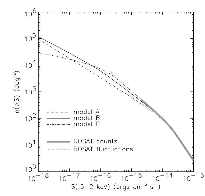
Figure 2: Integrated flux distributions for three extrapolated models of the XRB. Also shown are the ROSAT counts and fluctuation analysis limits from Hasinger et al. (1993).

Among the many possible models for the XRB, we consider only three cases: a model with a moderate slope half way between the fluctuation analysis limits (model B), and two extreme models with slopes at $S_{\rm ROSAT}$ just consistent with the fluctuation limits (models A and C). The second break was set at $S_{23}=2\times 10^{-16}$ ergs cm^-2 s^-1, close to the boundary of the fluctuation analysis limits. These three models are shown in figure 2. Their parameter values are given in table 1 along with those for the observed ROSAT number-flux relation which was modeled by Hasinger et al. (1993) as two broken power laws. The ROSAT counts are also displayed in the figure along with the fluctuation analysis limits. The moderate (B) and steep (C) models result in 100% of the XRB being produced by point sources alone. For the flat model (A), the contribution from point sources is only 77%, allowing for a small additional (e.g. diffuse) component of the XRB.

4 Effect of Lensing on the X-ray Background

4.1 General Results

We consider a region of the sky where the magnification due to gravitational lensing has a value $\mu$. The magnification has two effects on background point sources: their fluxes are magnified by factor of $\mu$ and their surface number density is diluted by the same factor. The observed flux and number density are,

$$S=\mu\hat{S}$$ (9)

and

$$n=\hat{n}/\mu,$$ (10)

where the unlensed quantities are denoted by a hat. Consequently, the observed differential number density is

$$\left.\frac{dn}{dS}\right|_{S}=\frac{1}{\mu^{2}}\left.\frac{d\hat{n}}{d\hat{S}}\right|_{S/\mu}.$$ (11)

When the unlensed flux distribution is a power law of the form $\left.({d\hat{n}/d\hat{S}})\right|_{\hat{S}}\propto\hat{S}^{-\beta}$, the observed counts follow $\left.({dn}/{dS})\right|_{S}\propto\mu^{\beta-2}{S}^{-\beta}$. Thus, the differential counts increase (decrease) as $\mu$ increases, if $\beta$ is above (below) the critical slope $\beta_{crit}\equiv 2$.

Since we ignore source clustering, the fluctuations in the number counts are solely due to Poisson statistics. The differential number of sources in a cell of solid angle $\Omega_{c}$ is $\left.({dN}/{dS})\right|_{S}=\Omega_{c}\left.({dn}/{dS})\right|_{S}$, and its differential variance is

$$\left.\frac{d\sigma^{2}_{N}}{dS}\right|_{S}=\Omega_{c}\left.\frac{dn}{dS}\right|_{S}.$$ (12)

Another useful quantity is the differential XRB intensity which is related to the differential counts through

$$\left.\frac{di}{dS}\right|_{S}=S\left.\frac{dn}{dS}\right|_{S}.$$ (13)

The differential intensity in a cell is $\left.({dI}/{dS})\right|_{S}=\Omega_{c}\left.({di}/{dS})\right|_{S}$, and its variance is

$$\left.\frac{d\sigma^{2}_{I}}{dS}\right|_{S}=S^{2}\Omega_{c}\left.\frac{dn}{dS}\right|_{S}.$$ (14)

It is often convenient to integrate these quantities between two observed fluxes, e.g. $n(S_{min},S_{max})\equiv\int_{S_{min}}^{S_{max}}dS\left.({dn}/{dS})\right|_{S}$. The limits $S_{min}=S_{r}$ and $S_{max}=\infty$ correspond to the resolved component of the XRB above the detection threshold $S_{r}$, and will be denoted hereafter as $n(>S_{r})$. The unresolved component corresponds to the limits $S_{min}=0$ and $S_{max}=S_{r}$, and will be denoted as $n(<S_{r})$.

By combining equation (11) with equations (12)–(14), we obtain the dependence of $n,\sigma_{N}^{2},i,$ and $\sigma_{I}^{2}$ on $\mu$. In particular, the total integrated intensity $i(0,\infty)=\int_{0}^{\infty}dSS\mu^{-2}\left.({d\hat{n}}/{d\hat{S}})\right|_{S/\mu}=\int_{0}^{\infty}d\hat{S}\hat{S}\left.({d\hat{n}}/{d\hat{S}})\right|_{\hat{S}}$, is invariant under magnification. This results from the conservation of the total surface brightness by gravitational lensing (e.g., Schneider et al. 1992, p. 132). However, the partial intensity $i(S_{min},S_{max})$ is not invariant under magnification, because the observed flux limits $(S_{min},S_{max})$ correspond to unlensed fluxes $(\hat{S}_{min},\hat{S}_{max})$ which depend on $\mu$.

It is interesting to note that the total intensity variance $\sigma_{I}^{2}(0,\infty)$, does depend on the magnification. Thus, gravitational lensing does not affect the mean intensity of the background but changes its angular fluctuations. Note that if $\beta<3$ (as is the case for counts in Euclidean space, where $\beta=\frac{5}{2}$), $\sigma_{I}^{2}$ does not converge as $S\rightarrow\infty$. In this case, the integrated intensity variance is only defined with respect to a given upper-limit on the flux.

4.2 Application to Lensing of Background X-ray Sources

We now apply the general relations discussed above to lensing of background X-ray sources. The solid line in figure 3 shows the unlensed relations ($\mu=1$) for the number density, intensity, and intensity variance for model B as a function of the 0.5–2 keV flux. The variance of the number density is not plotted since it is simply proportional to the number density (cf. Eq. [12]). The columns on the left and right hand side correspond to the differential and the integrated quantities, respectively. The resolved and unresolved integrated intensities are both plotted in panel (d), together with the total XRB intensity measured by ROSAT (Hasinger et al. 1993) which is shown as the dotted line. Panel (e) implies that, in this model, most of the XRB fluctuations originate from sources with fluxes between $\sim 10^{-16}$ and $5\times 10^{-13}$ ergs cm^-2 s^-1. For all models (and for the ROSAT counts; see discussion after Eq. [8]), $\beta_{1}=2.72$, i.e. smaller than 3. Therefore, the variance of the integrated intensity (cf. panel [f]), $\sigma_{I}^{2}(<S)$, diverges at bright fluxes but is well defined for a given upper-limit on the flux.

To illustrate the effect of magnification, figure 3 shows the various statistical quantities for $\mu=0.05$ (dot-dashed), 1 (solid), and 20 (dashed). Note that for $S<S_{*}\approx 10^{-15}$ ergs cm^-2 s^-1, the number of resolved sources $n(>S)$ decreases as $\mu$ increases (panel [b]). This so-called “magnification bias”, is a consequence of the fact that, at faint fluxes, the differential count slope $\beta$ is smaller than $\beta_{crit}$. However, the integrated intensity $i(>S)$ resolved above the same flux always increases when $\mu$ increases (panel [d]). Even though the magnification reduces the surface density of faint resolved sources, these sources appear brighter, and thus their integrated intensity increases. The integrated variance $\sigma_{I}^{2}(<S)$ of the unresolved intensity decreases when $\mu$ increases for $S<S_{*}$. However, the fluctuation $\sigma_{I}(<S)/I(<S)$ of the unresolved background (not shown on the figure) increases with $\mu$.

An inspection of figure 3 reveals that panel (d) is qualitatively different from panels (b) and (f) since it does not show any cross-over between the different magnification lines. In other words, $i(<S)$ always decreases with $\mu$ for all values of $S$. In appendix A, we show that this is generally true, to first order in $\mu-1$, for any unlensed number count relation $\left.{d\hat{n}}/{d\hat{S}}\right|_{\hat{S}}$, provided that the relevant integrated quantities converge. In the same appendix, we show that the cross-over flux $S_{*}$ for the weak lensing equivalent of panel (b) can be conveniently determined by comparing the solid lines in panels (b) and (c).

In summary, the magnification due to lensing effectively redistributes the intensity of the XRB into fewer but brighter sources, without altering the total intensity. For $S<S_{*}$ and for $\mu>1$, the number of resolved sources is decreased but their integrated intensity is increased. For the same flux limits, the unresolved XRB appears dimmer but with larger fluctuations.

We now consider the direct functional dependence of the various observable quantities on $\mu$. Figure 4 shows $n(>S_{r})$ as a function of $\mu$ for all three models. The detection threshold was fixed to $S_{r}(0.5-2\mbox{keV})=3\times 10^{-17}$ ergs cm^-2 s^-1. When considering the observability of the effect in practical cases [see §5.2 below], we will later take full advantage of the radial fall off of the cluster emission by adopting a variable detection threshold. Since $\beta_{3}<\beta_{crit}$ for all three models, $n(>S_{r})$ is a decreasing function of $\mu$ in all cases. The “knees” apparent for models B and C are due to the power law break at the flux $S_{23}$, which is shifted across the detection threshold by the magnification. With $\mu>1$, the relation is steepest for model C, and flattest for model A. This difference is primarily due to the different values of $(\beta_{3}-\beta_{crit})$ in these models, and can thus be used to observationally distinguish between these models.

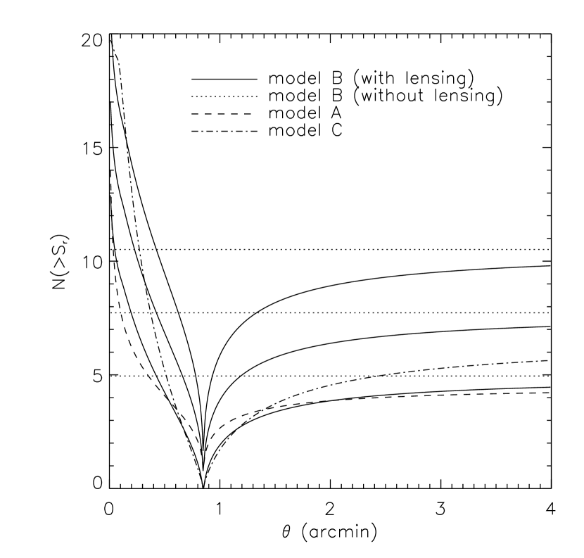
Figure 5: Radial dependence of the number of sources with fluxes above $S_{r}=3\times 10^{-17}$ ergs cm^-2 s^-1 in concentric annular cells with a solid angle of $\Omega_{c}=2$ arcmin². The three dotted lines correspond to the unlensed case. The three solid lines show the effect of lensing by a SIS with an Einstein angle of $\alpha=0^{\prime}.85$ for model B of the XRB. The central line in each set shows the mean number of sources, while the two outer lines correspond to a single Poisson standard deviation $\sigma_{I}$ away from the mean. The mean counts for models A and C are indicated by the dashed and dot-dashed curves, respectively.

By combining equations (4) and (11), one can derive the dependence of $N,I$ and $\sigma_{I}$ on the angle $\theta$ relative to the center of a SIS lens. As an example, figure 5 shows $N(>S_{r})$ as a function of $\theta$ for model B and for an annular cell size of $\Omega_{c}=2$ arcmin². The detection threshold was fixed to the value mentioned above and the Einstein radius $\alpha$ was chosen to be $0^{\prime}.85$, as in A1689. The unlensed case is shown as the dotted lines. In both cases, the central curve traces the mean count, while the two neighboring curves correspond to a single Poisson standard deviation $\sigma_{N}$ about the mean. The deficiency in the number of resolved sources close and beyond the Einstein radius is visible in the lensed case. For comparison, the mean lensed counts for models A and C are also shown. As expected, model C produces the steepest count profile. The observability of the source deficit will be discussed in §5.2.

It is instructive to examine the angular dependence of the resolved source counts at large radii. For $\theta\gg\alpha$, equation (4) yields $\mu\approx 1+\alpha/\theta$. For a sufficiently small detection threshold $S_{r}$, our three XRB models are dominated by the faint–end counts and thus $N(>S_{r})\approx\mu^{\beta_{3}-2}\hat{N}(>S_{r})$, where $\beta_{3}$ is the power law index at the faint end. As a result, $(N-\hat{N})\propto\hat{N}\theta^{-1}$. It is convenient to define the signal-to-noise ratio SNR_N relevant for distinguishing lensed from unlensed source counts as

$$\mbox{SNR}_{N}\equiv\frac{|N-\hat{N}|}{\sqrt{\hat{N}}}.$$ (15)

This quantity behaves as SNR${}_{N}\propto(\Omega_{c})^{\frac{1}{2}}\theta^{-1}$, where $\Omega_{c}$ is the solid angle of the annular observing cell with an angular radius $\theta$. Thus, one can keep SNR_N constant by choosing bins with $\Omega_{c}\propto\theta^{2}$. One can also define the signal-to-noise ratio SNR_I for separating the lensed intensity, $I(<S_{r})$, from the unlensed intensity $\hat{I}(<S_{r})$ of unresolved sources,

$$\mbox{SNR}_{I}\equiv\frac{|I-\hat{I}|}{\sqrt{\hat{I}}}.$$ (16)

Through a similar argument, SNR_I also maintains constancy for constant logarithmic bins of solid angle with $\Omega_{c}\propto\theta^{2}$.

4.3 Simulations

In order to substantiate the above analytic relations and to assess more realistically whether the lensing signal is detectable, we have performed numerical simulations of realistic X-ray observations. Our simulations generate a set of sources with random fluxes distributed according to the logN-logS relation for one of the XRB models. We include sources with fluxes in the range of $10^{-20}$ to $10^{-12}$ ergs cm^-2 s^-1 in the 0.5-2 keV band. This range is sufficiently broad to yield counts and intensities which are virtually indistinguishable from the ones expected in the full models. The sources were then assigned random positions in a square field of size $4^{\prime}\times 4^{\prime}$. For the lensed case, we considered a SIS lens with an Einstein angle $\alpha=0^{\prime}.85$, similar to that of A1689. The positions of the lensed images were derived from those of the unlensed sources by inverting equation (2), and their fluxes were computed using equations (4) and (9).

We then simulated observations of the lensed and unlensed fields with an X-ray imaging instrument for a given exposure time $t_{exp}$. We have adopted a Gaussian Point-Spread Function (PSF) with a one-dimensional standard deviation $\sigma_{psf}=0^{\prime\prime}.21$. The 0.5–2 keV flux to photon count rate conversion coefficient was taken to be $c^{\prime}=3.12\times 10^{11}$ cts ergs^-1 cm² s. These parameters correspond to the expected performance of the ACIS camera on board AXAF for 0.2–10 keV observations of sources with a spectral index $\gamma_{b}=0.4$ (see §5.1 below).

An example of the resulting photon maps for the unlensed and lensed cases is shown in figure 6. Here we have chosen the exposure time to be $t_{exp}=1\times 10^{6}$ s, and have adopted model B for the XRB. In order to improve the clarity of the picture, $\sigma_{psf}$ was degraded in this image to a value four times larger than that quoted in the previous paragraph. Note that the cluster emission is not shown on this image. The lensed photon map reveals a faint but noticeable ring close to the Einstein angle where sources are diluted. The presence of a few bright sources in this ring keeps its integrated intensity unchanged to within one standard deviation.

5 Observability

In this section, we discuss various strategies that could be adopted to search for the lensing effect in clusters. After discussing the relevant X-ray instrumentation of AXAF in §5.1, we consider the effect of lensing on the number counts of resolved sources in §5.2. An alternative approach involves measuring the unresolved intensity of the XRB below a given detection threshold, and is considered in §5.3. Finally, §5.4 summarizes other possible observing strategies.

5.1 X-Ray Instrument

The main limiting factors for observing the lensing effect are the cluster X-ray emission and the potentially low X-ray source density. Both of these limitations can be circumvented by using an instrument with a high angular resolution. Such an instrument would resolve faint sources even in the presence of the high effective background resulting from the cluster emission. The future Advanced X-ray Astronomy Facility (AXAF) mission (Elvis et al. 1995) is highly promising in this regard. The AXAF CCD Imaging Spectrometer (ACIS) camera on board the satellite has a projected PSF with a FWHM of about $0^{\prime\prime}.5$ (i.e. $\sigma_{psf}=0^{\prime\prime}.21$) and a pixel size of $0^{\prime\prime}.5$. For our purposes, we will ignore variations of the PSF across the field. The effective area of the instrument is 650 cm² at 1 keV. It is sensitive in the 0.2-8 keV band, and its field of view is $16^{\prime}\times 16^{\prime}$. The High Resolution Camera (HRC) in the same mission has a larger field of view, $32^{\prime}\times 32^{\prime}$, but a smaller effective area, 300 cm² at 1 keV. In this paper, we quote our results for the ACIS instrument because of its larger effective area.

Of particular interest is the detection capability of the AXAF-ACIS camera. In estimating its detection threshold, we consider a source detection scheme often used in X-ray surveys (e.g., Hamilton et al. 1991; Hasinger et al. 1993) which consists of counting photons inside a detection cell. The solid angle $\Omega_{c}$ of the detection cell is chosen to contain a substantial fraction $f_{p}$ of the total power of a point source placed at its center. Assuming Poisson statistics for the photons, the signal-to-noise ratio SNR_r for the resolution of a point source is then

$$\mbox{SNR}_{r}=\sqrt{t_{exp}}\frac{R_{s}}{\sqrt{R_{s}+R_{b}}},$$ (17)

where $t_{exp}$ is the exposure time, and $R_{s}$ and $R_{b}$ are the count rates in the detection cell produced by the source and the local background, respectively. The total background counts are generally the sum of the internal instrument background, the XRB, and the cluster emission. The exact count rate of the internal background is not currently available for the AXAF-ACIS camera, but is likely to be smaller than the cosmic XRB and therefore much smaller than the cluster emission. We therefore neglect the internal background in our calculation.

The flux threshold $S_{r}$ is related to $R_{s}$ by $S_{r}=cR_{s}f_{p}^{-1}$, where $c$ is a flux-to-count-rate coefficient which depends on the energy band, the instrument effective area, and the source spectrum. For the AXAF-ACIS camera and for sources with a spectral index $\gamma_{b}=0.4$ and $N_{H}=1.5\times 10^{20}$ cm^-2, the conversion coefficient in the 0.2-10 keV band is $c=7.39\times 10^{10}$ cts ergs^-1 cm². Of interest here is the conversion coefficient from fluxes in the 0.5–2 keV band into the AXAF count rate between 0.2–10 keV, which is $c^{\prime}=3.12\times 10^{11}$ cts ergs^-1 cm² for the same parameters.

The resulting flux detection threshold is plotted as a function of the signal-to-noise ratio in figure 8. Even though the detection occurs in the 0.2–10 keV band, the source fluxes are quoted in the more familiar 0.5–2 keV band. The fraction of the power in a detection cell was set to $f_{p}=0.96$. This corresponds to the PSF power contained in $2\times 2$ ACIS pixels. The solid line gives the AXAF detection performance for a background count rate equal to that of the XRB, i.e. for an observation in the field. The other curves correspond to increasing values of the background count rate in units of the XRB count rate. Note that, due to the degradation of the PSF, $S_{r}$ could be somewhat larger for sources observed off-axis. The presence of a high background level degrades the detection capabilities of the instrument. It is, however, striking that, for a background level equal to 600 times that of the XRB, the flux threshold at $2.5\sigma$ is only 4.3 times higher than that in the field. This relative insensitivity to the background level results from the high angular resolution of the AXAF telescope. Note that a zero background level corresponds to a curve which is virtually indistinguishable from the solid curve in figure 8, which corresponds to a background level equal to the XRB. Thus, the XRB (or equivalently, an internal background of comparable magnitude) has a negligible influence on the detection capabilities of this instrument.

5.2 Resolved Component

The simplest method to observe the lensing effect is to count the number of discrete sources at different radii about the cluster center. This technique is similar to that proposed by Broadhurst et al. (1995) in the optical band (see also Broadhurst 1995a,b). As shown in §4.2, the surface density of faint sources is expected to be diluted at radii beyond the Einstein angle of the cluster.

In searching for this dilution of faint sources, one can divide the field into concentric rings centered about the cluster center, and count the number of resolved sources in each ring above a given value of the detection signal-to-noise ratio, SNR_r. Note that, because of the variable level of cluster emission, the detection threshold $S_{r}$ for the fixed value of SNR_r depends on position (see figure 8). As discussed in §16, it is convenient to choose the ring areas so as to keep the source count signal-to-noise ratio SNR_N (Eq. [15]) constant. This is achieved by setting the area of each ring $R_{i}$ to be $\Omega_{r,i}=b\pi\theta_{i}^{2}$, where $\theta_{i}$ is the median radius of $R_{i}$ and $b$ is a dimensionless constant. The resulting ring radii will thus appear equally-spaced on a logarithmic angular scale.

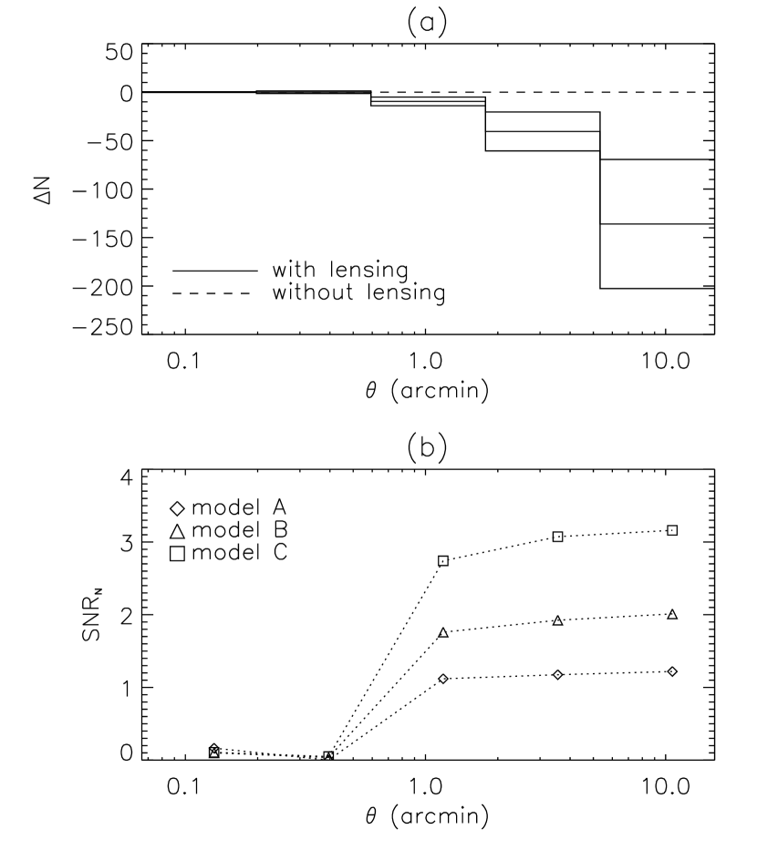
Figure 9: Effect of lensing on the resolved source counts for a $10^{6}$ s observation of A1689 with the AXAF-ACIS camera. For clarity, the angular range was extended to $\theta=16^{\prime}$, i.e. twice the field of view of this instrument. The source detection threshold was set to SNR${}_{r}=2$. The sources are binned in concentric rings centered about the cluster center with an area ratio of $b=8$. Panel (a) shows the source difference $\Delta N$ between the lensed and unlensed source counts for model B. The central solid line shows the mean count difference, whereas the two neighboring lines correspond to a single standard deviation $\sigma_{N}$ from the mean. The dashed line corresponds to $\Delta_{N}=0$, i.e. to an observation of the unlensed XRB. Panel (b) shows the signal-to-noise ratio SNR_N for separating the lensed from the unlensed counts. SNR_N is shown for each ring and for each of the three XRB models.

We present our results for the specific case of A1689. Figure 9a shows the expected difference $\Delta N\equiv N-\hat{N}$ between the lensed and unlensed detected source counts in each ring. This figure corresponds to a $t_{exp}=10^{6}$ s observation of this cluster with the AXAF-ACIS camera. Since we do not require a high accuracy in the position and fluxes of the detected sources, we took SNR_r to be as low as 2 . For the sake of clarity, we show the source counts from $\theta=0$ to $16^{\prime}$. This angular range could be covered by a mosaic of 4 adjacent $16^{\prime}\times 16^{\prime}$ ACIS images. In these calculations, we have adopted model B for the XRB. The lensing signal is generally maximized for a particular value of the ring area ratio $b$. In the case under consideration we adopted the optimal value of $b\approx 8$. The central solid line shows the mean count difference, whereas the two neighboring lines corresponds to a single standard deviation $\sigma_{N}$. The dashed line corresponds to the expected count difference in the absence of lensing, i.e. to $\Delta N=0$.

The deficit of lensed counts as compared to the unlensed counts is visible for the three outer rings with $\theta\gtrsim 0^{\prime}.6$. The cluster emission precludes the possibility of observing the lensing effect at smaller radii. Figure 9b shows the signal-to-noise ratio SNR_N for the difference between the lensed and the unlensed counts (Eq. [15]) in each ring. For model B, the three outer rings have values of SNR_N of 1.8, 1.9, and 2.0, from low to high values of $\theta$. In appendix B.1, we present a method for estimating the significance of the combined signal from several rings based on $\chi^{2}$ statistics. Using this method, we find that the combined source counts in the outer three rings at hand can be distinguished from the unlensed counts at the $2.9\sigma$ confidence level.

Figure 9b also shows the ring statistics for models A and C. Because of its flat faint logN-logS relation, model C produces the largest signal. The combined significance for the outer three rings is 1.8 and 4.8 for models A and C, respectively. The large difference between the combined significance of each model illustrates the sensitivity of the lensing effect to the XRB model.

If only one ACIS pointing is available, one can only count sources out to $\theta=8^{\prime}$. Since part of the most outer ring in figure 9 would then be lost, the lensing signal would be somewhat reduced. For the same conditions as quoted above but with $b=15$, only two rings then have a significant lensing signal. The combined significance of these two outermost rings is 1.7, 2.7, and $4.2\sigma$, for models A, B, and C, respectively.

We next examine the redshift dependence of the lensing signal by considering displaced versions of A1689 (see §2.3.2). Figure 10a shows the combined SNR_N as a function of the hypothetical cluster redshift $z_{l}$ for each of the XRB models. The figure corresponds to a $t_{exp}=10^{6}$ s observation with the AXAF-ACIS camera out to $\theta=16^{\prime}$ with SNR${}_{r}=2$ and $b=9$. All rings with an individual SNR_N greater than unity were included in the computation of the combined SNR_N. Notice that SNR_N is rather insensitive to the lens redshift in the range for $0.15\lesssim z_{l}\lesssim 0.6$. As the redshift of the cluster is increased, its Einstein angle decreases but so does the angular radius and surface brightness of its X-ray core. These competing effects tend to cancel each other. One can nevertheless notice that SNR_N peaks at a value of $z_{l}$ which depends on the XRB model; the peak value is reached at $z_{l}\approx 0.2$ for model C, and at $z_{l}\approx 0.4$ for model B. In model C, the lensing signal is stronger and thus the cluster emission is not as limiting as in the other models. As a result, it is advantageous in this model to position the cluster lens closer, thereby increasing the Einstein angle at the expense of stronger cluster emission. Note that if the faint background X-ray sources have a mean redshift substantially smaller than 1, then a non-negligible fraction of the XRB might be emitted in front of the distant clusters. In that case, figure 10a would need to be corrected for the reduction in SNR_N at high values of $z_{l}$.

Even though the detection of lensing through the change in the number counts of resolved X-ray sources requires a long exposure time with AXAF ($t_{exp}\sim 10^{6}$ s), the significance level of the signal is between 2 and $4\sigma$ in the case of A1689. The lensing effect can be used to probe the potential of rich clusters, especially at large radii. Since the amplitude of the effect is sensitive to the XRB model, a detection would constrain the faint end of the logN-logS relation for the background X-ray sources. The lensing signature on the resolved source counts is rather insensitive to the cluster redshift, and so many clusters with redshifts in the range $0.1\lesssim z_{l}\lesssim 0.6$ could have detectable signatures. Future systematic surveys of the lensing properties of X-ray clusters (see, e.g. Le Fèvre et al. 1994) could be used to optimize the selection of cluster lenses for this study.

5.3 Unresolved Component

5.3.1 Strategy

Because of the conservation of the total intensity by gravitational lensing (see §4.1), the resolved and unresolved background intensities are equivalent gauges of the lensing signal. However, in the presence of the strong cluster emission, the observational methods used to detect resolved point sources are significantly different from those used to measure unresolved intensities. It is therefore useful to examine the possibility of using the unresolved intensity as a complementary method for confirming the existence of the lensing effect.

The unresolved component of the XRB is contaminated by the cluster emission, whose radial profile is unknown a priori. However, at large radii, the cluster emission typically falls off rapidly as a power-law, $i_{c}\propto\theta^{-\beta_{x}}$, with $\beta_{x}\approx 5.19$ for the analytical fit used to model A1689 (Eq. [5]), or $\beta_{x}\approx 3$ for the King model (King 1962; Sarazin 1988). On the other hand, as far as the isothermal mass distribution applies, the signal-to-noise ratio of the lensing effect on the unresolved intensity falls–off only as $\theta^{-1}$ (Eq. [16]). The lensing effect could therefore dominate over the cluster emission at sufficiently large radii. As discussed in §4.2 (see also appendix A), lensing tends to reduce the unresolved intensity of the XRB. Consequently, the outer halo of a rich cluster might show an annulus where the diffuse X-ray intensity is lower than the sky-averaged intensity of the XRB, after the removal of resolved sources. In this sub-section, we will examine the detectability of this annulus, which is generic to lensing.

For this purpose, we divide, as before, the field into logarithmically-spaced concentric rings; this binning scheme keeps the signal-to-noise ratio of the unresolved intensity SNR_I (Eq. [16]) constant at large radii. After removing all the point sources with fluxes above a given flux detection threshold $S_{r}$, the unresolved background intensity can be measured in each ring. In a given ring, the total X-ray intensity is the sum of the XRB and the cluster emission intensities, $I_{tot}=I_{b}+I_{c}$. Here, we define the XRB intensity as $I_{b}(<S_{r})$ in the notation of §4.1. As noted in §5.1, the AXAF instrumental background is small compared to the cluster flux and can therefore be neglected.

Let us consider a ring $R$ of solid angle $\Omega_{c}$ and with a mean angular radius $\theta$. Typically, we consider a solid angle $\Omega_{c}\gtrsim 400$ arcsec², which is much larger than the PSF ($\pi\sigma_{psf}^{2}\approx 0.14$ arcsec²), and so we ignore the latter. The total photon counts in $R$ is then $P_{tot}=P_{b}+P_{c}$ with

$$P_{q}(\theta)\approx t_{exp}c_{q}\int_{R}d\Omega^{\prime}i_{q}(\theta^{\prime})$$ (18)

where $q=b,c$, $c_{q}$ are the appropriate flux-to-count rate conversion coefficients described in §1, and the integration extends over the solid angle of the ring $R$.

The variance of the photon counts $\sigma^{2}_{P,tot}$ can also be decomposed as $\sigma^{2}_{P,tot}=\sigma^{2}_{P,b}+\sigma^{2}_{P,c}$. Two effects contribute to $\sigma^{2}_{P,b}$: photon statistics and the intrinsic XRB fluctuations. These two effects are generally correlated since in a region of small intrinsic intensity, $P_{b}$ is small and thus the Poisson variance in the number of photons is small. However, for the long exposure time considered in this work, $P_{b}$ is very large, and so this correlation can be neglected. The variance of the XRB photon counts in $R$ is then

$$\sigma^{2}_{P,b}(\theta)\approx P_{b}+\left(t_{exp}c_{b}\right)^{2}\int_{R}d\Omega^{\prime}\sigma_{i,b}^{2}(\theta^{\prime}),$$ (19)

where the first term is due to photon statistics, and $\sigma_{i,b}^{2}\equiv\int_{0}^{S_{r}}dSS^{2}\left.({dn}/{dS})\right|_{S}$ is the intrinsic variance of the unresolved background intensity (see Eq. [14]). The variance in the cluster photon counts, $\sigma^{2}_{P,c}$, can also be decomposed into intrinsic and photon statistics terms. Given the strong cluster intensity and the geometry of the rings, the intrinsic term is probably small compared to the photon statistics term. We thus neglect the former term and approximate $\sigma^{2}_{P,c}\approx P_{c}$.

In order to characterize the strength of the lensing effect, we consider the difference $\Delta P\equiv P_{tot}-\hat{P}_{b}$, between the total number of counts observed ($P_{tot}$) and the expected number for the unlensed XRB counts ($\hat{P}_{b}$). The unlensed counts, $\hat{P}_{b}$, can be independently determined through an average over the entire sky, or through measurements of the unresolved intensity of the XRB in control regions which are far from any cluster. The lensing effect is expected to produce negative values of $\Delta P$. In order to assess the significance of this effect, we define the signal-to-noise ratio SNR_P for detecting a deficit in the photon counts as

$$\mbox{SNR}_{P}\equiv\frac{P_{tot}-\hat{P}_{b}}{\sigma_{P,tot}}=\frac{\Delta P}{\sigma_{P,tot}}.$$ (20)

5.3.2 Results

Figure 11a shows $\Delta P$ as a function of $\theta$ for model B. The count differences are shown for an AXAF-ACIS observation with $t_{exp}=10^{6}$ s of A1689 displaced to $z_{l}=0.6$. The ring area ratio was set to $b=0.8$. For clarity, this figure includes angles in the range $\theta=1$–$32^{\prime}$, implicitly requiring a mosaic of sixteen adjacent AXAF pointings. The detection threshold was set to $S_{r}(0.5-2\mbox{keV})=6\times 10^{-17}$ ergs cm^-2 s^-1. This threshold was chosen to optimize the lensing effect without removing too large a fraction of the XRB. The central solid line corresponds to the mean value of $\Delta P$. The two extreme solid lines correspond to one standard deviation $\sigma_{P,tot}$ away from the mean. The dashed line corresponds to $\Delta P=0$, i.e. to an observation of the unresolved XRB intensity outside the cluster.

The positive values of $\Delta P$ for $\theta\lesssim 10^{\prime}$ are, of course, due to the cluster emission. Lensing causes $\Delta P$ to take negative values for $\theta\gtrsim 10^{\prime}$, as long as the isothermal mass profile of the cluster extends out to these scales. As expected, the deficit in the unresolved XRB intensity only dominates at large angles, where the cluster emission is sufficiently weak.

Figure 11b shows SNR_P for each ring and for each XRB model. In rings with $\Delta P>0$, SNR_P was set to zero. For model B, the signal in the three outermost rings (taken separately) has a significance of SNR${}_{P}=$1.2, 1.4 and $1.4\sigma$, respectively. In appendix B.2, we describe a method for estimating the combined significance of the photon counts in several rings. Using this method, we obtain a combined significance of $2.0\sigma$ for the above three rings. The corresponding combined significances for models A and C are 1.79 and $2.06\sigma$, with $S_{r}(0.5-2\mbox{keV})=1\times 10^{-17}$ and $3\times 10^{-16}$ ergs cm^-2 s^-1, respectively. The minimum radius, $\theta_{\rm def}$, at which an intensity deficit is present (i.e. outside which $\Delta P<0$), is smallest in model C.

We can again study the redshift dependence of the lensing effect by considering different displacement redshifts $z_{l}$ for A1689 (see §2.3.2). Figure 10b shows the combined SNR_P as a function of $z_{l}$ for each of the XRB models. This figure corresponds to a $t_{exp}=1\times 10^{6}$ s observation with the AXAF-ACIS camera and $b=0.8$. In this plot the angles were restricted to the more realistic range of $0<\theta<16^{\prime}$, which corresponds to a mosaic of four adjacent AXAF-ACIS fields. The flux threshold was set to $S_{r}(0.5-2\mbox{keV})=1,6,30\times 10^{-17}$ ergs cm^-2 s^-1 for model A, B, and C, respectively. One readily notices that, for each model, SNR_P is equal to zero up to a redshift $z_{l,{\rm def}}$ beyond which it increases until it reaches a plateau. The value of $z_{l,{\rm def}}$ corresponds to the redshift at which $\theta_{\rm def}$ enters the field-of-view. At the actual redshift of A1689, none of the models produce a depletion. However, at $z_{l}=0.6$, the depletion is significant at the 1.1, 1.5 and $1.6\sigma$ level, for model A, B, and C, respectively. Note that these results are contingent on the validity of the isothermal sphere approximation out to the observed radii.

We conclude that it is more difficult to detect the lensing signature on the unresolved component of the XRB than it is in the resolved component case. However, it is qualitatively interesting that lensing could create an annulus around rich clusters where the diffuse unresolved X-ray intensity is smaller than its sky-averaged value. For clusters like A1689 observed with four adjacent AXAF-ACIS $10^{6}$s pointings, the depletion is present only for clusters with $z\gtrsim 0.5$ but with a low detection significance ($\sim 1-1.6\sigma$). The depletion would be much easier to detect behind clusters which are X-ray faint, such as hypothetical “dark” clusters with anomalously low gas fractions.

5.4 Other Observing Strategies

Another potential method for observing the lensing effect is to consider the angular fluctuations of the unresolved XRB. As shown in §4, magnification increases the fluctuations in the unresolved component of the XRB for $S<S_{*}$. Quantitatively, one could measure the unresolved integrated variance $\sigma_{I}^{2}(<S_{r})$ in concentric rings and attempt to detect an enhancement of the fluctuation $\sigma_{I}/I$ close to the Einstein radius. We leave the study of this approach to future work. A similar method using the auto-correlation function of the extragalactic background light was recently proposed for the optical band (Waerbeke et al. 1996; Waerbeke & Mellier 1996).

In this paper, we have only considered the detection of the lensing effect behind a single cluster, but an alternative approach could consist in combining X-ray observations of several clusters. One of the major limiting factors in detecting the lensing signal is the low number of resolved sources behind a single cluster. By stacking X-ray images of several clusters together, the effective number of resolved sources and the significance of the lensing signal would be increased. We have seen in §5.2, that the lensing signal for the resolved source counts is fairly insensitive to the cluster redshift. Therefore, any sufficiently massive cluster with $z_{l}$ between 0.1 and 0.6 could be used for this purpose. The significance of the signal could be maximized by rescaling the angular size of each cluster in units of its Einstein angle based on its X-ray temperature.

The same approach can, in fact, be carried one step further and applied to an all-sky survey which includes a large number of clusters and background sources. As shown in appendix A, the intensity of the unresolved component always decreases due to lensing. The cross-correlation between the unresolved XRB intensity and cluster positions on the sky is therefore expected to be reduced at large separations ($\sim 10^{\prime}$–$1^{\circ}$) due to lensing, while being enhanced at small separations due to X-ray emission by the clusters. A measurement of the cross-correlation function between Abell clusters and the ROSAT All-Sky Survey intensity was recently performed by Soltan et al. (1996). In a companion paper (Refregier & Loeb 1996b), we plan to examine the effect of lensing on such measurements.

Until now, we have modeled X-ray sources as point sources. However, as discussed in §3.1, some of the faint X-ray sources could be galaxies with extended emission and could thus produce lensed arcs. In order to derive a rough estimate for the probability of detecting an arc in A1689, we assume that a fraction $f_{e}$ of all X-ray sources are extended. We take the X-ray intensity of each extended source to be a disk with an intrinsic angular radius $\hat{\theta}_{e}$. Because of gravitational lensing, the apparent solid angle of a disk $\Omega_{e}$ is stretched by the magnification factor, i.e. $\Omega_{e}=\mu\hat{\Omega}_{e}$, where $\hat{\Omega}_{e}\equiv\pi\hat{\theta}_{e}^{2}$ is the unlensed solid angle. The source intensity is unchanged while the flux follows equation (9). We estimate the number $N_{arcs}$ of observable arcs to be the number of extended sources which are stretched by a factor larger than a given magnification, $\mu_{min}$, i.e.

$$N_{arcs}\approx f_{e}\int_{\mu>\mu_{min}}\!\!\!\!\!\!\!\!\!\!\!\!d\Omega\>n(>\!\!S_{r}(\theta)),$$ (21)

where the integration is over the region of the sky (typically a ring centered on the Einstein angle) in which $\mu>\mu_{min}$. After choosing a detection threshold SNR_r, the flux limit $S_{r}$ can be determined by inverting equation (17). Because we are now considering extended sources, the solid angle of the cell used for detecting sources must be set to $\Omega_{e}$ to encompass the total flux of the source. The value of $S_{r}$ depends on position because of the cluster emission.

Figure 12 shows the resulting expected number of arcs as a function of $\mu_{min}$ for different values of $\hat{\theta}_{e}$. The figure corresponds to a $10^{6}$ s observation of A1689 with the AXAF-ACIS camera. In this plot, we assume a detection threshold of SNR${}_{r}=3$ and adopt model B for the XRB. At a given value of $\mu_{min}$, the number of arcs which can be resolved is smaller for intrinsically larger sources because of the cluster emission. Note, however, that such sources produce larger arcs for a given value of $\mu_{min}$. For $\hat{\theta}_{e}=1^{\prime\prime}$ and for $\mu_{min}=3$, the expected number of arcs is comparable to $f_{e}$.

6 Conclusions

In this work we have analyzed the gravitational lensing signature of a single rich cluster of galaxies on the XRB. We have found that near and outside the Einstein angle of the cluster (i.e. for $\theta\gtrsim 1^{\prime}$), lensing results in a deficit of resolved X-ray sources with fluxes $\gtrsim 3\times 10^{-17}~{}{\rm ergs~{}cm^{-2}~{}s^{-1}}$. In the same region, the corresponding unresolved component of the XRB appears dimmer and more anisotropic. Although the lensing signal peaks near the Einstein angle of the cluster (cf. Fig. 5), its detection is easier in the outer regions where the cluster emission is negligible.

For concreteness, we have considered future observations of the cluster A1689 with the forthcoming AXAF-ACIS camera. After a $10^{6}$ second exposure on this instrument, a detection of the lensing signature imprinted on the resolved background source counts should be difficult but possible out to $8^{\prime}$ from the center of A1689 with a significance level of $\sim 2$–$4\sigma$, depending on the choice of the extrapolated flux distribution of faint X-ray sources (see Fig. 9). Far from the cluster core ($\theta\gtrsim 10^{\prime}$), the deficit in the unresolved intensity of the XRB due to lensing may dominate over the intensity excess due to the cluster emission. For X-ray bright clusters, it is, however, difficult to detect this deficit (cf. Figs. 10 and 11).

The main factors affecting the strength of the lensing signal are the size of the Einstein angle and the intensity of the cluster emission. Massive clusters typically have large Einstein radii, but also tend to have high X-ray luminosities (see, e.g. Sarazin 1988). The lensing signature on the resolved source counts is almost insensitive to the lens redshift in the range $0.1\lesssim z_{l}\lesssim 0.6$ (cf. Fig. 10). Existing surveys of the X-ray properties of clusters (eg. Ebeling et al. 1996) can be used, in conjunction with simplifying assumptions (such as spherical symmetry, relation between velocity dispersion X-ray temperature), to select the most promising clusters for this study. Future systematic surveys of the lensing properties of X-ray clusters (see, e.g. Le Fèvre et al. 1994) will provide increased confidence in the selection of these clusters.

Currently, little is known observationally about the mass distribution on scales $\sim 10^{\prime}$ around clusters. Far from the cluster center, the lensing signal-to-noise ratio behaves as $\theta^{-1}$ and thus falls–off more slowly than the cluster free-free intensity, which typically decreases at least as rapidly as $\theta^{-3}$. X-ray telescopes with a large field of view could therefore probe the mass distribution as far as the virialization boundary of a cluster, well outside the regime where the X-ray emission from the cluster is detectable.

Because the magnification bias due to lensing is sensitive to the faint end slope of the number-flux relation of X-ray sources, the amplitude of the lensing signal can constrain different models of the extrapolations of this relation (cf. Figs. 2 and 9). Deep X-ray imaging of cluster fields may be used in this way to shed more light on the origin of the XRB.

The nature of the faint population of extragalactic X-ray sources is still a matter of debate. In most of this work, we have assumed that all sources are high–redshift AGN and would thus appear point-like. However, it is possible that a significant fraction, $f_{e}$, of them are associated with extended emission from distant galaxies (Jones et al. 1995; Boyle et al. 1995; Carballo et al. 1995; Griffiths et al. 1996; however see Hasinger 1996a,b; Refregier et al. 1996). The existence of extended sources behind the lensing cluster can be tested by a search for X-ray arcs or arclets. For a $10^{6}$ second observation of A1689 with AXAF-ACIS, the number of arclets which are stretched by a factor $\gtrsim 3$ and are detectable at the $3\sigma$ level, is roughly comparable to $f_{e}$ for intrinsic source sizes $\sim 1^{\prime\prime}$ (see Fig. 12). The statistical detection of weak distortions to the intrinsic ellipticities of sources is routinely done in optical studies of weak lensing (Schneider 1995; Kaiser 1995; and Narayan & Bartelmann 1996), and could also be extended, although with smaller statistics, to the X-ray band. By observing an ensemble of lensing clusters, it may therefore be possible to calibrate the contribution of narrow-emission-line galaxies at high redshift to the XRB.

In the future, we plan to extend the present single cluster analysis and include the effect of lensing by an ensemble of clusters (Refregier & Loeb 1996b). The effect of lensing on the cross-correlation between clusters and the unresolved intensity of the XRB is particularly interesting in light of a recent measurement of the correlation between Abell clusters and the ROSAT All-Sky Survey (Soltan et al. 1996). Lensing reduces the intensity of the unresolved background (cf. appendix A), and thus provides a negative contribution to the cross-correlation signal at large angular separations ($\sim 10^{\prime}$–$1^{\circ}$), where the cluster emission is negligible.

Appendix A Qualitative Effects of Magnification

In this appendix, we address the question whether the resolved source counts $n(>S)$ and the unresolved intensity $i(<S)$ decrease or increase as the magnification $\mu$ increases. The results are not only applicable to the XRB, but also hold for any background consisting of a collection of randomly distributed point sources which are sufficiently distant from the lens.

For the purpose of this discussion, it is convenient to rename the unlensed differential counts as $f(\hat{S})\equiv\left.({d\hat{n}}/{d\hat{S}})\right|_{\hat{S}}$ (see notation in §4.1). We also rewrite the magnification as $\mu=1+\epsilon$, and consider the weak lensing regime in the outer parts of the lensing cluster where $\epsilon\ll 1$.

A.1 Resolved Source Counts

The resolved lensed counts above a flux threshold $S$ is $n(>S)=\int_{S}^{+\infty}dS^{\prime}\mu^{-2}f(S^{\prime}\mu^{-1})$ (see Eq. [11]). After expanding in powers of $\epsilon$ and integrating by parts, we obtain, to first order in $\epsilon$,

$$n(>S)\approx\hat{n}(>S)-\epsilon\left[\hat{n}(>S)-\left.\frac{d\hat{i}}{d\hat{S}}\right|_{S}\right],$$ (A1)

where we have used the unlensed version of equation (13). The tendency of $n(>S)$ to increase or decrease with $\mu$ therefore depends on the sign of the quantity in brackets. This sign can be conveniently determined by comparing the solid line in figure 3b with that in figure 3c. A cross-over between the solid and the weak lensing equivalent of the dashed and dot-dashed lines in figure 3b will occur at any values of $S=S_{*}$ for which $\hat{n}(>S_{*})=\left.({d\hat{i}}/{d\hat{S}})\right|_{S_{*}}$. This result holds for any function $f(\hat{S})$, as long as $\hat{n}(>S)$ converges.

A.2 Unresolved Intensity

We now turn to the unresolved intensity which, in our notation, is $i(<S)=\int_{0}^{S}dS^{\prime}S^{\prime}\mu^{-2}f(S^{\prime}\mu^{-1})$ (see Eq. [13]). As before, an expansion in powers of $\epsilon$ and an integration by parts yields to leading order in $\epsilon$,

$$i(<S)\approx\hat{i}(<S)-\epsilon\left[\left.\frac{d\hat{\sigma}_{i}^{2}}{d\hat{S}}\right|_{S}\right],$$ (A2)

where $\left.({d\hat{\sigma}_{i}^{2}}/{d\hat{S}})\right|_{S}\equiv S^{2}f(S)$ (see Eq. [14]). In analogy with equation (A1), the quantity in bracket in equation (A2) involves a higher moment, namely $\left.({d\hat{\sigma}_{i}^{2}}/{d\hat{S}})\right|_{S}$, which can be determined from the solid line in figure 3e. However, the quantity in brackets in equation (A2) does not contain a term analogous to the first term in the bracket of equation (A1). This is due to a cancellation which is unique to $i$. In general, we may consider any integrated quantity $g$ of the form $g(S_{1},S_{2})\equiv\int_{S_{1}}^{S_{2}}dSS^{\lambda}\left.({dn}/{dS})\right|_{S}$, where $\lambda$ is a constant. It then follows that the cancellation will occur only for $\lambda=1$, i.e. for $g\equiv i$. This feature of $i$ is also responsible for the conservation of the total integrated intensity $i(0,\infty)$ under magnification, which was discussed in §4.1. As a result, the quantity in square brackets in equation (A2) is positive definite, and so $i(<S)$ always decreases as $\mu$ increases. Magnification always causes sources to appear brighter and thus allows a larger fraction of the background to be resolved. Consequently, no cross-over occurs between the solid and dot-dashed or dashed lines in figure 3d.

A similar analysis shows that the above cancellation does not occur for $\sigma_{i}^{2}(<S)$ (corresponding to $\lambda=2$). Cross-overs are allowed in this case, as shown in figure 3f. Again, these results are valid for any function $f(\hat{S})$ as long as the integrated intensity and variance converge.

Appendix B Count Statistics

B.1 Source Counts

In this appendix, we evaluate the statistical significance of the lensed source counts as compared to the unlensed counts. Let us consider source counts in $n_{R}$ concentric rings $R_{j},j=1,\dots,n_{R}$ centered on the cluster center. We denote the mean number of sources in $R_{j}$ as $\overline{N}_{j}$ and $\hat{\overline{N}}_{j}$ in the lensed and unlensed case, respectively.

In a single experiment, one measures the number of sources $N_{j}$ in each ring $R_{j}$. The variable $N_{j}$ follows a Poisson distribution with mean $\overline{N}_{j}$ and $\hat{\overline{N}}_{j}$, in the lensed and unlensed case. The mean unlensed counts $\{\hat{\overline{N}}_{j}\}$ can be determined from a large-area observation of the XRB “in the field” (i.e. away from any cluster) with an accuracy which is effectively arbitrary, and can thus be treated as well determined constants. We want to test and possibly rule out the hypothesis that the measured counts $\{N_{j}\}$ were drawn from the unlensed distribution. For this purpose, we treat each ring as an independent measurement and consider the following statistic in a single experiment

$$X^{2}_{\rm single}(N_{k};\hat{\overline{N}}_{k})\equiv\sum_{j=1}^{n_{R}}\frac{(N_{j}-\hat{\overline{N}}_{j})^{2}}{\hat{\overline{N}}_{j}}.$$ (B1)

Since the considered distributions are Poisson and not Gaussian, it is not guaranteed that $X^{2}_{\rm single}$ follows a $\chi^{2}$ distribution. Numerical simulations reveal, however, that, for our experimental conditions, $X^{2}_{\rm single}$ does follow this distribution to a good approximation. This is true even when $n_{R}$ is as low as 2 and when $\hat{\overline{N}}_{k}$ is as low as 4. In our case, we can thus derive likelihood probabilities using the usual $\chi^{2}$ tables.

Our probability estimate is obtained by averaging $X^{2}_{\rm single}$ over a large number $n_{E}$ of experiments. If we denote by $N_{k,e}$ the source count in $R_{k}$ for the e^th experiment, the mean statistic is

$$X^{2}(\overline{N}_{l};\hat{\overline{N}}_{l})\equiv\frac{1}{n_{E}}\sum_{e=1}^{n_{E}}X^{2}_{\rm single}(N_{k,e},\hat{\overline{N}}_{k}),$$ (B2)

which can be easily evaluated numerically.

As an example, let us consider the third, fourth and fifth rings in figure 9 which we rename as $R_{1}$, $R_{2}$, and $R_{3}$, respectively. In this case, $\overline{N}_{1}\approx 19.3$, $\overline{N}_{2}\approx 404.4$, and $\overline{N}_{3}\approx 4426.7$, whereas $\hat{\overline{N}}_{1}\approx 28.7$, $\hat{\overline{N}}_{2}\approx 444.8$, and $\hat{\overline{N}}_{3}\approx 4561.7$. Note that although $\mu\propto\theta^{-1}$ at large angles, the values of $\hat{\overline{N}}_{i}$ do not follow a geometric sequence because of the variable detection threshold (see §5.2). By numerically averaging over $n_{E}=10^{3}$ experiments, we obtain $X^{2}\approx 13.38$. The $\chi^{2}$-probability to exceed this value is about 99.61% for 3 degrees of freedom. The lensed counts determined in a single experiment are thus, on average, distinguishable from the unlensed counts at the $2.9\sigma$ significance level.

B.2 Photon Counts

In this section, we quantify the significance of the reduction in the photon counts due to lensing after the resolved sources have been removed. For this purpose, let $\overline{P}_{j}$ be the mean of the total number of photons (i.e. the sum of the cluster emission and the lensed unresolved XRB) in a ring $R_{j}$, and let $\sigma_{P,j}$ be the associated standard deviation. The number of photons expected in the same ring for the unlensed unresolved XRB is denoted by $\hat{\overline{P}}_{j}$.

Again, we first consider a single experiment in which $P_{j}$ photons are detected in the ring $R_{j}$. Here, a useful statistic to consider is

$$X^{2}_{\rm single}(P_{k};\sigma_{P,k};\hat{\overline{P}}_{k})\equiv\sum_{j=1}^{n_{R}}\frac{(P_{j}-\hat{\overline{P}}_{j})^{2}}{\sigma_{P,j}^{2}}.$$ (B3)

In general, the distributions of the variables $P_{j}$ are not Gaussian. We have indeed seen in §5.3 that their distribution results from a combination of intrinsic background fluctuations and photon shot noise for both the cluster and XRB contributions. In our case, however, the mean photon counts are large (typically $\overline{P}_{k}\gtrsim 2\times 10^{4}$ for the outer rings) and the distribution is close to Gaussian. We can therefore take $X^{2}_{\rm single}$ to be distributed as a $\chi^{2}$-variable with $n_{R}$ degrees of freedom.

If we perform a large number $n_{E}$ of experiments and denote by $P_{k,e}$ the photon counts in $R_{k}$ for the e^th experiment, then the mean statistic is

$$X^{2}(\overline{P}_{l};\sigma_{P,l};\hat{\overline{P}}_{l})\equiv\frac{1}{n_{E}}\sum_{e=1}^{n_{E}}X^{2}_{\rm single}(P_{k,e};\sigma_{P,k};\hat{\overline{P}}_{k}).$$ (B4)

As an example, let us rename the ninth, tenth, eleventh ring in figure 11 as $R_{1}$, $R_{2}$, and $R_{3}$, respectively. In this case, $\overline{P}_{1}\approx 34621$, $\overline{P}_{2}\approx 62696$, $\overline{P}_{3}\approx 112693$, $\hat{\overline{P}}_{1}\approx 35189$, $\hat{\overline{P}}_{2}\approx 63556$, $\hat{\overline{P}}_{3}\approx 113879$, $\sigma_{P,1}\approx 468$, $\sigma_{P,2}\approx 631$, $\sigma_{P.3}\approx 846$. This results in $X^{2}\approx 8.43$, which corresponds to a $\chi^{2}$ probability of 96.2% for 3 degrees of freedom. The total lensed photon counts in a single experiment are thus, on average, below the unlensed XRB with a significance of $2.0\sigma$.

Table 1: Parameters for models of the logN-logS relation for X-ray sources.

	Model A	Model B	Model C	ROSAT
$\eta_{1}\tablenotemark{b}$	1.98e-22	1.98e-22	1.98e-22	1.98e-22
$\eta_{2}\tablenotemark{b}$	7.45e-09	9.36e-11	4.11e-12	7.68e-12
$\eta_{3}\tablenotemark{b}$	7.45e-09	1.13e-06	9.19e+01	–
$\beta_{1}$	2.72	2.72	2.72	2.72
$\beta_{2}$	1.72	1.86	1.96	1.94
$\beta_{3}$	1.72	1.60	1.10	–
$S_{12}\tablenotemark{c}$	2.66e-14	2.66e-14	2.66e-14	2.66e-14
$S_{23}\tablenotemark{c}$	2.00e-16	2.00e-16	2.00e-16	2.50e-15
%XRB	77%	100%	100%	–

Figure 1: Einstein angle $\alpha$ as a function of source redshift $z_{s}$ for a SIS. The Einstein angle is scaled by $\sigma_{1500}\equiv\sigma_{v}/(1500$ km s${}^{-1})$, where $\sigma_{v}$ is the 1D velocity dispersion. The solid and dashed lines correspond to a cosmological density parameter of $\Omega=1$ and 0.2, respectively. The lines from left to right correspond to lens redshifts of $z_{l}=0.1,0.2$ and 0.3, respectively.

Figure 3: Flux distributions for: (a,b) the number density $n$ of X-ray sources; (c,d) the mean XRB intensity $i$; and, (e,f) the variance $\sigma_{I}^{2}$ of the XRB flux $I$ for a cell of solid angle $\Omega_{c}=1$ deg². The results are for model B of the XRB. We show the unlensed distributions ($\mu=1$) together with the apparent distributions for a magnified ($\mu=20.$) and a de-magnified ($\mu=.05$) region of the sky. Differential and integrated quantities are shown on the left and right columns, respectively. In panel (b) the integration limits are from $S$ to $\infty$ (resolved component), whereas in panel (f) the limits are from 0 to $S$ (unresolved component). In panel (d), both the resolved and unresolved distributions are shown as the decreasing and increasing curves, respectively. The invariant total XRB intensity (Hasinger et al. 1993) is shown as the dotted line on the same panel.

Figure 4: Dependence of the resolved source density $n(>S_{r})$ on the magnification $\mu$ for a detection threshold of $S_{r}(0.5-2\mbox{keV})=3\times 10^{-17}$ ergs cm^-2 s^-1. Results are plotted for each of the three XRB models.

Figure 6: Simulated photon maps for model B sources with 0.5-2 keV fluxes in the range of $10^{-20}$ to $10^{-12}$ ergs cm^-2 s^-1. The detector parameters are those expected for the AXAF-ACIS camera. However, for clarity we used $\sigma_{psf}$ which is four times larger than expected. The exposure time is $10^{6}$ sec. The maps correspond to: (a) unlensed sources; and (b) sources lensed by a SIS with $\alpha=0^{\prime}.85$, the Einstein angle of A1689.

Figure 6b: [See caption on previous page]

Figure 8: Estimated detection capability of the AXAF-ACIS camera. Detection flux thresholds are plotted as a function of the source signal-to-noise ratio. The detection is performed in the 0.2–10 keV band. However, fluxes are quoted in the more familiar 0.5–2 keV band. The dependence on the exposure time $t_{exp}$ was factored out. The solid line represents an observation in the field, i.e. with the background equal to the XRB. The other lines correspond to different background count rates in units of the XRB count rate in the 0.2–10 keV band, as measured by Gendreau et al. (1995).

Figure 10: Dependence of the lensing signal on the cluster redshift. Several values of the redshift $z_{l}$ of a displaced version of A1689 are considered for each of the XRB models, and for a $10^{6}$ s observation with the AXAF-ACIS camera. For clarity, the angular range was extended to $\theta=16^{\prime}$, i.e. to twice the field of view of this instrument. Panel (a) shows the combined SNR_N for resolved source counts expected for SNR${}_{r}=2$ and $b=9$. Panel (b) shows the combined SNR_P of the photon counts for the unresolved intensity. We chose $b=3$ and set the detection flux threshold to $S_{r}(0.5-2\mbox{keV})=1,6,30\times 10^{-17}$ ergs cm^-2 s^-1 for model A, B and C, respectively.

Figure 11: Effect on lensing on the unresolved component of the XRB for a $10^{6}$ s observation of A1689 with the AXAF-ACIS camera. For clarity, the angular range was extended to $\theta=32^{\prime}$, i.e. to four times the field of view of this instrument. The flux detection threshold was set to $S_{r}(0.5-2\mbox{keV})=1,6,30\times 10^{-17}$ ergs cm² s^-1 for model A, B, and C, respectively, and $b$ was set to a value of 0.8 . Panel (a) shows the photon count difference $\Delta P$ for model B. The central solid line shows the mean count difference, whereas the two neighboring lines correspond to a single standard deviation $\sigma_{P,tot}$ away from the mean. The dashed line corresponds to $\Delta P=0$, i.e. to an observation of the (unlensed) XRB “in the field”. Panel (b) shows the signal-to-noise ratio SNR_P for each ring and for each XRB model.

Figure 12: Expected number of arcs $N_{arcs}$ as a function of the minimum magnification (or stretch) factor $\mu_{min}$ for several intrinsic source sizes $\hat{\theta}_{e}$. The fraction $f_{e}$ of extended sources in the population of X-ray sources was factored out on the vertical axis. The results correspond to a $10^{6}$ s observation of A1689 with the AXAF-ACIS camera, and a source detection threshold of SNR${}_{r}=3$. We assume model B for the XRB.

References

- (1) Arnaud, M., Forman, W. F., Jones, C., Hughes, J. P. H., 1994, preprint
- (2) Allen, S. W., Fabian, A. C., & Kneib, J. P., 1996, MNRAS, 279, 615
- (3) Bartelmann, M., & Steinmetz, M. 1996, preprint astro-ph/9603101
- (4) Bahcall, N. A., & Cen, R. 1994, ApJL, 426, L15
- (5) Boyle, B. J., Griffiths, R. E., Shanks, T., Stewart, G. C., & Georgantopoulos, I., 1993, MNRAS, 260, 49
- (6) Boyle, B. J., McMahon, R. G., Wilkes, B. J., & Elvis, M., 1995, MNRAS, 272, 462
- (7) Briel, U. G., & Henry, J. P. 1994, Nature, 372, 439
- (8) Broadhurst. T. J., Taylor, A. N., & Peacock, J. A., 1995, ApJ, 438, 49
- (9) Broadhurst. T. J., 1995a, in Proc. of the 5th Maryland Dark Matter conference, Oct. 1994. available as astro-ph/9505010
- (10) Broadhurst. T. J., 1995b, preprint, astro-ph/9511150
- (11) Cen, R., Kang, H., Ostriker, J. P., Ryu, D., 1995, ApJ, 451, 436
- (12) Carballo, R., et al., 1995, MNRAS, 277, 1312
- (13) Cen, R., & Ostriker, J. P. 1994, ApJ, 429, 4
- (14) Chen, L. W., Fabian, A. C., & Gendreau, K. C., preprint, astro-ph/9511089
- (15) Daines, S., Jones, C., Forman, W., & Tyson, A., 1996, ApJ, submitted
- (16) De Zotti, G., Toffolatti, L., Franceschini, A., Barcons, X., Danese, L., & Burigana, C. 1995. in Proc. of the International School of Space Science 1994 course: X-Ray Astronomy. ed G. Bignami et al. in preparation.
- (17) Ebeling, H., Voges, W., Böhringer, H., Edge, A. C., Huchra, J. P., & Briel, U. G., 1996, MNRAS, 281, 799
- (18) Eke, V. R., Cole, S., & Frenk, C. S. 1996, preprint astro-ph/9601088
- (19) Elvis, M. et al. 1995, The AXAF Science Instrument Notebook, available at http://hea-www.harvard.edu/asc/SIN /SIN.html
- (20) Fabian, A. C., & Barcons, X. A. 1992, ARA&A, 30, 429
- (21) Fixsen, D. J., Cheng, E. S., Gales, J. M., Mather, J. C., Shafer, R. A., & Wright, E. L. 1996, preprint astro-ph/9605054
- (22) Forman, W., & Jones, C., 1982, ARA&A, 20, 547
- (23) Forman, W., & Jones, C. 1990, in Clusters of Galaxies, ed. W. R. Oegerle, M. J. Fitchett, & L. Danly (Cambridge Univ. Press: Cambridge), 257
- (24) Fox, D., & Loeb, A. 1996, in preparation
- (25) Giacconi, R., Gursky, H., Paolini, F., & Rossi, B., 1962, Phys. Rev. Lett., 9, 439
- (26) Gendreau, K. C., et al., 1995, PASJ, 47, L5
- (27) Griffiths, R. E., Della Ceca, R., Georgantopoulos, I., Boyle, B. J., Stewart, G. C., Shanks, T., & Fruscione, A. 1996, MNRAS, 281, 71
- (28) Hamilton, T. T., Helfand, D. J., & Wu, X., 1991, ApJ, 379, 576
- (29) Hasinger, G., Burg, R., Giacconi, R., Hartner, G., Schmidt, M., Trümper, J., & Zamorani, G., A&A, 275, 1.
- (30) Hasinger, G., 1996a, in Examining the Big Bang and Diffuse Background Radiations, eds Kafatos, M., & Kondo, Y. (Netherlands: IAU), 245
- (31) Hasinger, G., 1996b, in Proc. of Röntgenstrahlung from the Universe, MPE report 263, eds. Zimmermann, H. U., Trümper, J. E.,& Yorke, H. (Germany: MPE), p. 291
- (32) Henriksen, M. & Markevitch, M. 1996, preprint astro-ph/9604150
- (33) Henry, J. P., & Briel, U. G. 1995, ApJ, 443, 9
- (34) Inoue, H., Kii, T., Ogasaka, Y., Takahashi, T., & Ueda, Y., 1996, in Proc. of Röntgenstrahlung from the Universe, MPE report 263, eds Zimmermann, H. U., Trümper, J. E.,& Yorke, H. (Germany: MPE), p. 323
- (35) Jones, L. R., et al., 1995, in Proc. of the 35th Herstmoncieux Conference: Wide-Field Spectroscopy and the Distant Universe, eds Maddox, S., & Aragon-Salamanca, A. (Singapore: World Scientific Publishing)
- (36) Kaiser, N. 1995, preprint astro-ph/9509019
- (37) King, I. R., 1962, AJ, 67, 471
- (38) Kneib, J. P., & Soucail, G., 1996, in Proc. of the 173rd IAU Symposium: Astrophysical Applications of Gravitational Lensing, eds. Kochanek, C. S., & Herwitt, J. N. (Boston: Kluwer Academic)
- (39) Kochanek, C. S. 1992, ApJ, 384, 1
- (40) Le Fèvre, O., Hammer, F., Angonin, M. C., Gioia, I. M., & Luppino, G. A., 1994, ApJ, 422, L5
- (41) Loeb, A., & Ostriker, J. P. 1992, Institute for Advanced Study preprint, IAS-AST/92
- (42) Loeb, A., & Mao, S. 1994, ApJ, 435, L109
- (43) Markevitch, M. 1996, ApJ, 500, L1
- (44) Markevitch, M., Mushotzky, R., Inoue, H., Yamashita, K., Furuzawa, A., & Tawara, Y. 1996, ApJ, 456, 437
- (45) Mather, J. C., et al., 1990, ApJ, 354, L37
- (46) Miralda-Escudé, J., & Babul, A., 1995, ApJ, 449, 18
- (47) Narayan, R., & Bartelmann, M. 1996, Lectures held at the 1995 Jerusalem Winter School, preprint astro-ph/9606001
- (48) Neumann, D. M., & Böhringer H. 1996, submitted to MNRAS, preprint astro-ph/9607063
- (49) Refregier, A., Helfand, D. J., & McMahon, R. G., 1996, submitted to ApJ
- (50) Refregier, A., & Loeb, A. 1996a, in Proc. of Röntgenstrahlung from the Universe, MPE report 263, eds Zimmermann, H. U., Trümper, J. E.,& Yorke, H. (Germany: MPE), p. 611
- (51) Refregier, A., & Loeb, A. 1996b, in preparation
- (52) Richstone, D., Loeb, A., & Turner, E. 1992, ApJ, 393, 477
- (53) Sarazin, C. L., 1988, X-Ray Emissions from Clusters of Galaxies. (Cambridge: Cambridge Univ. Press)
- (54) Schneider, P. 1995, preprint astro-ph/9512047
- (55) Schneider, P., Ehlers, J., & Falco, E. E., 1992, Gravitational Lenses. (New York: Springer-Verlag)
- (56) Soltan, A. M., Hasinger, G., Egger, R., Snowden, S., & Trümper, J. 1996, A & A, 305, 17
- (57) Squires, G., Kaiser, N., Babul, A., Fahlman, G., Woods, D., Neumann, D., & Böhringer, H. 1996a, ApJ, 461, 572
- (58) Squires, G., Kaiser, N., Fahlman, G., Babul, A., & Woods, D. 1996b, ApJ, submitted, preprint astro-ph/9602105
- (59) Teague, P. F., Carter, D., & Gray, P. M., 1990, ApJS, 72, 715
- (60) Tyson, J. A., Valdes, F., & Wenk, R. A., 1990, ApJ, 349, L1
- (61) Tyson, J. A., & Fischer, P., 1995, ApJ, 446, L55
- (62) Van Waerbeke, L., Mellier, Y., Schneider, P., Fort, B., & Mathez, G. 1996, A&A, in press. available as astro-ph/9604137
- (63) Van Waerbeke, L., & Mellier, Y., 1996, preprint, astro-ph/9606100
- (64) Vikhlinin, A., Forman, W., Jones, C., & Murray, S., 1995a, ApJ, 451, 542
- (65) ——, 1995b, ApJ, 451, 553
- (66) ——, 1995c, ApJ, 451, 564
- (67) Weisskopf, M. C., et al. 1987, Astroph. Lett. & Commun., 26, 1
- (68) Zamorani, G. 1995. in Background Radiation Meeting (1993). ed Calzetti, D., et al. (Cambridge: Cambridge Univ. Press)