Bloated Stars as AGN Broad Line Clouds:
The Emission Lines Response to Continuum Variations

Abstract

The ‘Bloated Stars Scenario’ proposes that AGN broad line emission originates in the winds or envelopes of bloated stars (BS). Alexander and Netzer (1994, 1996) established that $\sim 5\mbox{$\times$}10^{4}$ BSs with dense, decelerating winds can reproduce the observed emission line spectrum and line profiles while avoiding rapid collisional destruction. Here, I investigate a third prediction of the model, related to the size of the broad line region, by deriving the emission line response to variations in the ionizing continuum (‘line reverberation’) and comparing it to observations. The expected time lags, as well as the order of response of the various lines, strongly depend on the typical variability time scale of the ionizing continuum. The BS model studied here corresponds to a bright Syfert 1 galaxy (Sy1) or a low luminosity QSO. I find that the BS model is consistent with the observed correlation between the Balmer lines time lags and the AGN luminosity, which at present is the only line reverberation information available for this luminosity class. The model displays also some of the anti-correlation between the time lags of the metal emission lines and their degree of ionization that has been observed in a few low-luminosity Sy1s. However, the bright Sy1 model results differs from the low-luminosity Sy1 data in that the ${\rm H}\beta$ time lag is relatively shorter and the ${\rm C}\,{\sc iv}\,\lambda 1549$ time lag relatively longer.

1 Introduction

The observed properties of active galactic nuclei (AGN) lead to the conclusion that the broad line emission originates in numerous small, cold and dense gas concentrations, which are photoionized by the central continuum source. These objects are labeled “clouds”, although their true nature remains unknown. A basic challenge for any broad line region (BLR) model is to specify the physical mechanism that protects the clouds from rapid disintegration in the AGN’s extreme environment, or else specify a source for their continued replenishment. The bloated stars (BSs) model [Edwards 1980, Mathews 1983, Scoville & Norman 1988, Penston 1988, Kazanas 1989] proposes that the lines are emitted from the winds or mass loss envelopes of giant stars. The star provides both the gravitational confinement and the mass reservoir for replacing the gas that evaporates from the envelope to the interstellar medium (ISM). The BS model is further motivated by the lack of observational evidence for net radial motion in the BLR (e.g. Maoz et al. 1991, Wanders et al. 1995). This is consistent with virialized motion in the gravitational potential of the nucleus.

The BS model was recently studied by Alexander & Netzer [Alexander & Netzer 1994] (paper I) and Alexander & Netzer [Alexander & Netzer 1996] (paper II), which used a detailed photoionization code to calculate the emission line spectrum and profiles of various BS wind models. The integrated emission line spectrum was calculated by combining the line emissivity of the BSs with theoretical models of the stellar distribution function. The model results were compared to the mean AGN line ratios and to estimates of the BLR size and line reddening. The mean observed ${\rm Ly}\alpha$ equivalent width was used to determine the number of BSs and their fraction in the stellar population and to estimate the collisional mass loss rate and its effect on the ISM electron scattering optical depth. Detailed models of the stellar velocity field were then used to derive the line profiles, which in turn constrained the BS distribution within the stellar population.

The main result of papers I and II is that there are BS wind models that can reproduce the emission line ratios and profiles to a fair degree with only a small fraction of BSs in the stellar population. However, these models do not resemble winds of normal supergiants. The photoionization calculations show that the emission line spectrum is dominated by the conditions at the outer boundary of the line emitting zone of the wind. The successful BS models are those with dense envelopes that have small density gradients. In this case, the wind boundary is set by tidal forces near the black hole and by the finite mass of the wind at larger radii. Only $\sim 5\mbox{$\times$}10^{4}$ such BSs ($<1\%$ of the BLR stellar population) are required for reproducing the BLR emission. As a result, the collision rate is reasonably small ($<1\mbox{$M_{\odot}$}$/yr). On the other hand, lower-density wind models or those with steep density gradients are ruled out because they emit strong broad forbidden lines, which are not observed in AGN. In addition, their low line emissivity requires orders of magnitude more BSs in the BLR. This leads to rapid collisional destruction, very high mass loss rate and very short BS lifetimes. Even if the BSs are continuously created, the ISM electron scattering optical depth is very large, contrary to what is observed.

Paper II shows that in order to reproduce the typical shapes and widths of the observed emission line profiles it is necessary to assume that the BS fraction in the stellar population falls off as $r^{-2}$. The emerging picture is that AGN harbour an exotic class of giant stars, whose existence is linked to the uniquely violent environment of AGN, and are consequently much rarer in the more usual stellar environments outside the inner nucleus. There are at least two astronomical precedences for such a situation: The existence of blue stragglers in the high density cores of stellar clusters, which is thought to be linked to stellar mergers or collisions (e.g. Bailyn 1995) and the recently discovered concentration of extremely rare He i blue giants in the inner 1 pc of the Galactic Center [Krabbe et al. 1991]. The envelopes of these blue giants reach densities as high as those assumed in the BS model [Najarro et al. 1996].

The present work explores a third aspect of the BS model: BLR line reverberation, or echo mapping. The continuum luminosity of AGN is observed to vary in time and in many cases, the continuum variability pattern is echoed after some time lag by the line fluxes. This is considered the most direct support for the photoionization hypothesis of BLR emission. The time lag between the continuum and line variations is interpreted as the difference between the light travel time along the direct line of sight and that along the indirect path from the continuum source, via the line emitting gas, to the observer. The continuum and line light curves are therefore related by the spatial emissivity distribution (‘emissivity map’) of the line, which in turn depends on the distribution of line emitting objects and their ionization structure.

Extracting information on the BLR geometry from line reverberation data is severely limited by observational difficulties and the ensuing ambiguities in the statistical analysis (e.g. Maoz 1994). A reliable analysis requires good sampling over a long period, a condition which is seldom met. Only a few monitoring campaigns were carried out to date, each with a different duration and sampling frequency. In contrast to the case of the line ratios and profiles, very little can be determined at this stage about the statistics of the time lags and their properties. However, some general trends are beginning to emerge: the BLR size seems to be positively correlated with the continuum luminosity, and high ionization metal lines seem to originate at smaller radii than the low ionization ones [Clavel et al. 1991].

In this third part of the work I study the line reverberation properties of a BS model with a luminosity of a bright Seyfert 1 galaxy (Sy1) or a low-luminosity QSO. This model succeeded in reproducing the line ratios and profiles of a typical AGN, and here I check whether it is also consistent with the limited available line reverberation data. Section 2 briefly summarises the main components of the BS model. Section 3 describes the line reverberation simulation procedure. The simulated results are presented in section 4 and discussed in section 5.

2 The BS model

As described in detail in papers I and II, t he BS model is specified by two main ingredients. The stellar distribution around the black hole and the density structure of the BS envelope. The BS model that is discussed in this paper is model C of paper II.

The stellar distribution function that I use is based on the numeric results of Murphy, Cohn & Durisen [Murphy, Cohn & Durisen 1991] (MCD), which follow the evolution of a spherically symmetric multi-mass coeval stellar cluster in the presence of a central black hole. The black hole mass grows as it accretes mass from the stars, both directly, by tidal disruption, and indirectly, from mass loss in the course of stellar evolution and of inelastic stellar collisions. While the calculations deal in a self-consistent way with the stellar dynamics and the build-up rate of the central mass, the resulting AGN luminosity is not well defined. This is because the calculations of the nucleus evolution are insensitive to the properties of the central mass, such as the ratio between the black hole mass and the infalling mass or to the black hole’s angular momentum, nor are they affected by the details of the accretion mechanism or by the rest-mass to luminosity conversion efficiency, $\eta$. MCD make the simple assumption that the bolometric luminosity is $L_{\rm bol}(t)=\eta\dot{M}(t)c^{2}$ with $\eta=0.1$, where $\dot{M}$ is the total stellar mass loss rate from the stellar system. In this work I use MCD model 2B, at $t_{0}=10^{9}$ yr, when the black hole mass is $\mbox{$M_{\rm bh}$}=1.9\mbox{$\times$}10^{8}\mbox{$M_{\odot}$}$, and the ionizing luminosity $L_{\rm ion}=3.6\mbox{$\times$}10^{44}$ erg s^-1. This luminosity is sub-Eddington and is determined by the total mass loss rate from the stellar system. This evolved system represents a luminous Sy1 or a low-luminosity QSO. Once the choice of the stellar model is made, the remaining free parameters are $f_{\rm\/BS}$, the fraction of BSs in the normal stellar population and the inner and outer radii of the BLR, $r_{\rm in}$ and $r_{\rm out}$. In paper II, it was shown that these parameters are constrained by the observed emission line profiles to values of roughly $\mbox{$r_{\rm in}$}=0.001$ pc, $\mbox{$r_{\rm out}$}=0.25$ pc, and $\mbox{$f_{\rm\/BS}$}\propto r^{-2}$, with the BSs comprising less than 1% of all stars.

A single BS is modeled by a simplified, spherically symmetric structure with no claim to hydrodynamical self-consistency and without specifying the process that drives the wind. It has two components: a giant star of radius $\mbox{$R_{\star}$}=10^{13}$ cm and a mass of $\mbox{$M_{\star}$}=0.8\mbox{$M_{\odot}$}$, emitting a spherically symmetric wind at a rate of $\mbox{$\dot{M}_{\rm w}$}=10^{-6}\mbox{$M_{\odot}$}$/yr. The wind, or envelope, extends to a radius $R_{\rm w}$ which contains an additional mass of up to $\mbox{$M_{\rm w}$}=0.2\mbox{$M_{\odot}$}$. The wind density is parameterized as a power-law, with two free parameters

$$N(R)=\mbox{$N_{\star}$}(R/\mbox{$R_{\star}$})^{-\beta}\,,$$ (1)

where $N_{\star}$ is the hydrogen number density at the base of the envelope. The combined constraints of the observed line ratios and profiles fix these parameters to values of roughly $\beta=3/2$ and $\mbox{$N_{\star}$}=3.8\mbox{$\times$}10^{11}$ cm^-3. The proximity of the BSs to the black hole makes tidal disruption the main physical mechanism that limits the size of the wind. For example, at 30 ld, the BS wind radius (model C) is $\mbox{$R_{\rm w}$}\sim 2\mbox{$\times$}10^{14}$ cm.

The BS model is fully specified by the choice of the AGN dynamical age, $t_{0}$, which fixes $M_{\rm bh}$, by the BS structure and the ionizing continuum spectrum. However, tidally-limited BSs obey certain approximate scaling relations that link $N_{\star}$ and $L_{\rm ion}$ in a way that allows $L_{\rm ion}$ and $N_{\star}$ to be jointly modified without affecting the emissivity map (paper II). Since the emissivity map determines the line ratios and profiles, this scaling property means that the model luminosity cannot be currently fixed by either the BS model or the MCD AGN model. This introduces some uncertainty in matching the BS model with observed AGN that complicates the comparison of the model time lags with the observed ones (section 5).

3 Calculations

In order to calculate the light curves of the various emission lines it is necessary to specify the line response to the local changes in the ionizing flux. A commonly assumed simplification is that the response is linear, in which case the relation between the line light curve, $L(t)$, and the ionizing continuum light curve $C(t)$ can be described by a convolution with a transfer function $\Psi$ [Blandford & McKee 1982]

$$L(t)=\int_{-\infty}^{+\infty}C(\tau)\Psi(t-\tau)d\tau\,.$$ (2)

In the case of a spherically symmetric BLR the transfer function is [Maoz et al. 1991]

$$\Psi(t)\propto\left\{\begin{array}[]{lrcl}0,&&t&<0\\[5.0pt] \int_{\mbox{$r_{\rm in}$}}^{\mbox{$r_{\rm out}$}}w(r)c/2rdr,&0\leq&t&<2\mbox{$r_{\rm in}$}/c\\[5.0pt] \int_{ct/2}^{\mbox{$r_{\rm out}$}}w(r)c/2rdr,&2\mbox{$r_{\rm in}$}/c\leq&t&<2\mbox{$r_{\rm out}$}/c\\[5.0pt] 0,&2\mbox{$r_{\rm out}$}/c\leq&t&\end{array}\right.$$ (3)

The weight $w(r)$ is the normalized line emissivity from a shell of BSs at radius $r$,

$$w(r)=r^{2}\mbox{$n_{\rm\/BS}$}(r)L_{\ell}(r)\left/\int_{\mbox{$r_{\rm in}$}}^{\mbox{$r_{\rm out}$}}r^{2}\mbox{$n_{\rm\/BS}$}(r)L_{\ell}(r)dr\,,\right.$$ (4)

where $L_{\ell}(r)$ is the BS emissivity in line $\ell$ at a distance $r$ from the continuum source and $n_{\rm\/BS}$ is the BS spatial density. $w(r)$ is calculated by the photoionization code for the specific BS model. The assumption of a linear response implicitly includes the approximation that the varying continuum does not change the emissivity map of the BLR, i.e. that $\Psi$ is unaffected by $C(t)$. While this is not strictly true (the ionization parameter is proportional to the ionizing flux), it is probably an adequate approximation as long as the variations are not large. Another way of interpreting $\Psi(t)$ is that it is the line response to a $\delta$-function continuum flash.

Figure 1: The transfer functions $\Psi(t)$ of various lines as calculated for model C. $\Psi$ is normalized to 1 at $t=0$.

As is the standard practice in the field of line reverberation studies, I identify the time lag between the two light curves with the peak in their cross-correlation function (CCF) [Blandford & McKee 1982].

4 Results

The present calculations demonstrate the general behaviour of the BS system by describing in detail a particular model that was investigated in paper II. This model (model C) is characterized by a relatively low $\mbox{$L_{\rm ion}$}/\mbox{$M_{\rm bh}$}$ ratio ($3.6\mbox{$\times$}10^{44}$ erg s^-1 / $1.9\mbox{$\times$}10^{8}\mbox{$M_{\odot}$}$), a BS fraction in the stellar population that decreases like $r^{-2}$ and a relatively low hydrogen density at the base of the wind ($3.8\mbox{$\times$}10^{11}$ cm^-3). I calculated the transfer functions of various emission lines, which are displayed in Fig. 1, by inserting the photoionization results for model C into equations 2 and 3.

There is a distinct difference between the transfer functions of the high ionization lines ${\rm He}\,{\sc ii}\,\lambda 1640$ and ${\rm O}\,{\sc vi}\,\lambda 1035$, and that of the low ionization line ${\rm Mg}\,{\sc ii}\,\lambda 2798$. This reflects the fact that in this model, the high ionization lines are formed at the inner BSs, where the ionizing flux is high, whereas the low ionization lines are formed further away from the continuum source, where the lowered ionizing flux allows the existence of extended, partially ionized regions in the BS envelope. This trend resembles what is found in line reverberation campaigns, namely that the high ionization metal lines have shorter time lags than the low ionization metal lines.

The time lag of a line increases with the width of its transfer function. However, the relative widths of the transfer function give only a rough indication of the rank order of the line lags. The time lag of an extended BLR geometry, such as that of model C, depends also very strongly on the time-scale of the ionizing continuum, because the line CCF is the convolution of $\Psi$ with the continuum auto-correlation function [Penston 1991, Netzer 1991]. I check this here by calculating the response of the lines to Gaussian shaped continuum flashes of various durations (parameterized by their standard deviation $\sigma$). Figure 2 shows two such flashes with duration of $\sigma=10$ and 100 d, respectively, and the responses of the ${\rm Ly}\alpha$ and ${\rm Mg}\,{\sc ii}\,\lambda 2798$ lines. As expected, the narrow, $\sigma=10$ d flash induces a line light curve very similar in shape to its transfer functions and consequently, the two light curves respond quickly at lags of 20 d and 32 d, respectively. On the other hand, the wide, $\sigma=100$ d flash results in noticeably larger time lags of 84 d and 120 d, respectively, and a larger lag difference between the two lines.

The response times of various lines as a function of the Gaussian pulse width are summarized in Fig. 3. Note that even for pulses as wide as $\sim 1$ year, most of the line lags continue to increase with the continuum time-scale. Only the responses of ${\rm H}\beta$ and ${\rm O}\,{\sc vi}\,\lambda 1035$ appear to begin to saturate. The different rates of time lag increase result in the surprising effect that not only the time-lags, but also their rank order, changes with increasing continuum variability time scale. For example, the ${\rm H}\beta$ line, which lags after the ${\rm O}\,{\sc vi}\,\lambda 1035$ and ${\rm He}\,{\sc ii}\,\lambda 1640$ lines when the ionizing continuum varies quickly, precedes these lines when the continuum varies slowly. In some lines the time lag is a steep function of the continuum variability timescale. For example, the ${\rm He}\,{\sc ii}\,\lambda 1640$ line time lag increases by a factor of 6 when the width of the continuum flash is increased by a factor of 18. Although I demonstrated these trends only in the case of one particular BS model and single Gaussian flashes, I expect these results to hold also in the general case. This is because all BS models have extended BLR geometries and all realistic continuum light curves can be approximated, to some degree, by a superposition of Gaussian flashes.

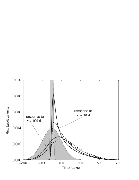
Figure 2: The response of the model C ${\rm Ly}\alpha$ (bold line) and ${\rm Mg}\,{\sc ii}\,\lambda 2798$ (dashed bold line) lines to narrow ($\sigma=10$ d) and wide ($\sigma=100$ d) Gaussian flashes (shaded areas), which are centered on t = 0.

Figure 3: The response of various model C lines to Gaussian shaped continuum flashes, as a function of the Gaussian standard deviation $\sigma$.

A realistic ionizing continuum is made up of many peaks of different widths. I model this by using the recently obtained long light curve of PG0844 (Kaspi 1996, private communication). Figure 4 shows the smoothed observed PG0844 optical continuum and the response of the ${\rm He}\,{\sc ii}\,\lambda 1640$ and ${\rm Mg}\,{\sc ii}\,\lambda 2798$ lines. The lags were calculated without the first 100 days of the line light curves, which is roughly the time it takes $\Psi$ to fall to half its initial maximal value. At times shorter than that, the line light curve depends strongly on the preceding, unobserved continuum and cannot be calculated reliably. Note the difference between the lines response to the wide second continuum peak and their response to the narrow third peak. This is the pattern of behaviour that was suggested by the simulations with single Gaussian flashes and by the simulations of Pérez, Robinson & de la Fuente [Pérez, Robinson & de la Fuente 1992]. Such a behaviour was actually observed in the 1989 NGC 5548 IUE campaign [Netzer & Maoz 1990]. Table 1 lists the lags of all the lines calculated here. As with the Gaussian flashes, there is an anti-correlation between the time lag and the degree of ionization.

Line	lag (days)	rank order
${\rm Ly}\alpha$	70	3
${\rm H}\alpha$	75	4
${\rm H}\beta$	60	1
${\rm He}\,{\sc i}\,\lambda 5876$	70	3
${\rm He}\,{\sc ii}\,\lambda 1640$	65	2
${\rm C}\,{\sc iii}\,\lambda 977$	75	4
${\rm C}\,{\sc iii]}\,\lambda 1909$	80	5
${\rm C}\,{\sc iv}\,\lambda 1549$	80	5
${\rm N}\,{\sc v}\,\lambda 1240$	70	3
${\rm O}\,{\sc vi}\,\lambda 1035$	60	1
${\rm Mg}\,{\sc ii}\,\lambda 2798$	95	6

Table 1: The calculated lags (CCF peaks) of Model C for the smoothed continuum light curve of PG0844, shown in Fig. 4. The CCF was calculated without the first 100 days of the line light curve. The CCF is calculated with a 5 day resolution. The rank order of the lags (1 is the shortest) is also displayed for convenience.

Figure 4: The response of model C ${\rm He}\,{\sc ii}\,\lambda 1640$ and ${\rm Mg}\,{\sc ii}\,\lambda 2798$ lines to the smoothed 4759Å (rest frame) continuum of PG0844 (Kaspi 1996, private communication). In order to make the comparison between the light curves easier, the displayed line light curves are shifted to the continuum mean and their variation is scaled up to the continuum r.m.s variation.

5 Discussion

In papers I and II, it was shown that the BS model can successfully account for two main features of AGN spectra: the emission line ratios and their profiles. Here, I study the line reverberation of the BS model and check whether it can also account for this aspect of AGN properties. I focus on the two trends that emerge from the available observational results: the positive correlation between the AGN luminosity and the typical time lag scale and the anti-correlation between the line time lag and its degree of ionization.

Several difficulties stand in the way of a direct comparison of the BS model predictions with observed line reverberation results. From the observational side, the picture is still unclear since the available sample of adequately sampled AGN is small and spans only a limited range in luminosity. A reliable statistical analysis of the time lags is notoriously difficult, and this is compounded by the fact that the quoted time lags in the various campaigns were derived by a variety of statistical procedures, each with its own biases. The strong dependence of the time-lag on the characteristic continuum variability is another factor that has yet to be taken into account.

From the theoretical side, there is the difficulty that there is some degeneracy among the BS model parameters that makes it possible to have similar emissivity maps for different luminosities (see section 2), and therefore the luminosity of this AGN model is not well defined. This was not a serious problem for comparing the BS model line ratios and profiles with the the observed ones, because observationally, these do not appear to be strongly correlated with the AGN luminosity [Netzer 1990]. This is not the case with the time lag results, as there is an indication of a correlation between the time lag and luminosity [Maoz 1994, Kaspi et al. 1996b].

To date, published time lag results, which are based on the Balmer lines, exist only for 9 AGN (NGC 5548 [Korista et al. 1995]; NGC 4151 [Kaspi et al. 1996a, Maoz et al. 1991]; NGC 3227 [Salamanca et al. 1994]; NGC 3783 [Stirpe et al. 1994a]; AKN 120 [Peterson et al. 1988, Peterson & Gaskell 1991]; MRK 279 [Maoz et al. 1990, Stirpe et al. 1994b]; NGC 3516 [Wanders et al. 1993]; MRK 590 [Peterson et al. 1993]; NGC 4593 [Dietrich et al. 1994]). These AGN have estimated luminosities in the range $6.5\mbox{$\times$}10^{42}$ to $1.8\mbox{$\times$}10^{44}$ erg s^-1 and ${\rm H}\beta$ time lags in the range 4 to 28 d. This sample suggests a weak positive correlation between the luminosity and the ${\rm H}\beta$ time lag. A major improvement in testing this correlation is offered by new results from a line reverberation campaign on a sample of QSO with luminosities from $4\mbox{$\times$}10^{44}$ to $3\mbox{$\times$}10^{46}$ erg s^-1. Preliminary estimates of the time lags confirm that the correlation is indeed real and yield ${\rm H}\beta$ time lags of approxiamtely 100 d for the luminosity range 2 to $5\mbox{$\times$}10^{45}$ erg s^-1 [Kaspi et al. 1996b].

Because it is possible that some of the correlation between the time lag and luminosity is caused by a correlation between the continuum variability time scales and the luminosity, I use in the simulations the optical continuum of PG0844 (one of the QSO in this new sample), which is close in its luminosity to that of model C. In doing so, I am assuming that the ionizing light curve is similar to the optical one. The luminosity of PG0844, when estimated by the same procedure as above, is $4.7\mbox{$\times$}10^{44}$ erg s^-1 and that of model C is $2.3\mbox{$\times$}10^{44}$ erg s^-1. I thus expect the lag of model C to be intermediate between those of the observed Sy1 sample (lags $\la 30$ d for $L\la 2\mbox{$\times$}10^{44}$ erg s^-1) and those of the new QSO sample (lags $\sim 100$ d for $L\sim 4\mbox{$\times$}10^{45}$ erg s^-1). The model ${\rm H}\beta$ and ${\rm H}\alpha$ lags of 60 and 75 d, respectively, (Table 1) indeed place it in this intermediate range (as do the time lags of all the other lines). Thus, the time lag of BS model C is consistent with these observations.

The BS model time lags display to some extent the trend for an inverse correlation between the lag and the degree of ionization (‘time lag line segregation’), which is observed in a few low-luminosity Sy1s. Two groups of lines can be identified among the 11 broad emission lines which were calculated. The relatively high ionization species, ${\rm He}\,{\sc ii}\,\lambda 1640$, ${\rm N}\,{\sc v}\,\lambda 1240$ and ${\rm O}\,{\sc vi}\,\lambda 1035$, have narrower transfer functions and shorter lags than the relatively low ionization species, ${\rm C}\,{\sc iii}\,\lambda 977$, ${\rm C}\,{\sc iii]}\,\lambda 1909$ and ${\rm Mg}\,{\sc ii}\,\lambda 2798$ (Fig. 1 and table 1). There are two notable differences between the model results and the observations. The ${\rm C}\,{\sc iv}\,\lambda 1549$ has a large time lag, which is comparable to those of the low ionization lines and the ${\rm H}\beta$ has a short time lag, comparable to that of the high ionization lines.

There are reasons to suspect that line reverberation time lags of low-luminosity AGN can not be simply extrapolated to higher luminosities. The results presented in Fig. 3 suggest that any detailed ordering of the line time lags, especially those with short time lags, strongly depends on the typical variability time scales of the ionizing continuum. This may explain the seeming ${\rm C}\,{\sc iv}\,\lambda 1549$ discrepancy. The ${\rm H}\beta$ discrepancy may also be related to the “${\rm Ly}\alpha/{\rm H}\beta$ problem”. All photoionization models of the BLR consistently under-predict the Balmer lines emission. This is one of the outstanding problems in AGN research, which remains unsolved despite extensive efforts. The most likely explanation is a combination of reddening and inaccurate treatment of the line transfer, which arises from the local nature of the escape probability method. This simplified approach may be inadequate for the extreme ${\rm Ly}\alpha$ and ${\rm H}\alpha$ optical depths that are typical of the BLR. Detailed line transfer calculations, which deal separately with the different frequency bins in the line profiles, are needed (see Netzer 1990 for a review). Such calculations are beyond the scope of this paper. This situation casts doubt on the reliability of the calculated model ${\rm H}\beta$ time lags. Note, however, that the agreement between the model time lag scale and the observed time lag–luminosity correlation does not hang only on the ${\rm H}\alpha$ and ${\rm H}\beta$ time lags but is also supported by the time lags of the other lines.

The time lag line segregation of the BS model is not as pronounced as that found in the NGC 5548 campaign [Clavel et al. 1991, Peterson et al. 1991, Dietrich et al. 1993]. A similar trend is also seen with respect to the line profiles. The observed profiles display line to line differences (‘profile line segregation’), which is more pronounced than that of the model. This may indicate that the BS fraction is even more centrally concentrated than the assumed $\mbox{$f_{\rm\/BS}$}\propto r^{-2}$.

This rough agreement of the model with the observations reinforces two of the conclusions that followed from the line profile study in paper II. The line segregation in the profile widths and time lags is yet another indication that the BSs can not be Comptonized (paper I). Comptonization implies that the BS wind boundary is determined by the ionizing flux and is at a constant ionization parameter, irrespective of the distance from the black hole. This leads to similar emissivity maps for all lines and hence to similar profiles and lags, contrary to what is observed. The line profiles and lags also require that the fraction of BSs in the stellar population, $f_{\rm\/BS}$, fall off at least as $r^{-2}$. A less concentrated BS distribution results in significantly larger lags. For example, BS model B of paper II, which is identical to model C apart for having $\mbox{$f_{\rm\/BS}$}={\rm const.}$, yields a ${\rm H}\beta$ lag of 210 d for the PG0844 continuum. This is in clear contradiction with the observations.

In this paper I studied one particular BS model (model C), which is specified by a particular choice of the AGN dynamical age, the BS envelope structure and the ionizing spectrum. Other choices of these parameters will result in other model predictions. This work is part of a series of feasibility studies aimed at checking whether one BS model can simultaneously reproduce the main broad line properties of a typical AGN. Model C was shown to reproduce the line ratios and line profile, and was therefore also in the focus of this line reverberation study. Direct comparison of model C with observed line reverberation time lags must await future monitoring campaigns of bright Sy1s. The question whether a BS model of a low-luminosity Sy1 is consistent with the detailed line reverberation data available on such AGN is part of the larger question of whether the BS model can be extended to the full range of observed AGN luminosities. This will be explored in a future paper. In the meanwhile, I conclude that BS models, similar to those discussed here, are consistent with current line reverberation data on AGN in the bright Sy1 / low-luminosity QSO range.

Acknowledgments

I am very grateful to Hagai Netzer for his advice and careful reading of the draft. Shai Kaspi’s help and permission to use unpublished results are much appreciated. This research was partially supported by the Israel Science Foundation administered by the Israel Academy of Sciences and Humanities and by the Jack Adler chair of Extragalactic Astronomy at Tel Aviv University.

References

- [Alexander & Netzer 1994] Alexander T., Netzer H., 1994, MNRAS, 270, 781 (Paper I)
- [Alexander & Netzer 1996] Alexander T., Netzer H., 1996, MNRAS, submitted (Paper II)
- [Bailyn 1995] Bailyn C. D., 1995, ARA&A, 33, 133
- [Blandford & McKee 1982] Blandford R. D., McKee C. F., 1982, ApJ, 209, 214
- [Clavel et al. 1991] Clavel J. et al., 1991, ApJ, 366, 64
- [Dietrich et al. 1993] Dietrich, M. et al., 1993, ApJ, 408, 416
- [Dietrich et al. 1994] Dietrich, M. et al., 1994, A&A, 284, 33
- [Edwards 1980] Edwards A. C., 1980, MNRAS, 190, 757
- [Kaspi et al. 1996a] Kaspi S. et al., 1996a, ApJ, 470, 336
- [Kaspi et al. 1996b] Kaspi S., Smith P. S., Maoz D.,Netzer H., Januzzi B. T., 1996b, ApJL, 471, 75
- [Kazanas 1989] Kazanas D., 1989, ApJ, 347, 74
- [Korista et al. 1995] Korista K. T., et al., 1995, ApJS, 97, 285
- [Krabbe et al. 1991] Krabbe A., Genzel R., Drapatz S., Rotaciuc V., 1991, ApJL 382, L19
- [Maoz et al. 1990] Maoz D. et al., 1990, ApJ, 351, 75
- [Maoz et al. 1991] Maoz D. et al., 1991, ApJ, 367, 493
- [Maoz 1994] Maoz D., 1994, in Gondhalekar P. M., Horne K., Peterson B. M., eds, Reverberation Mapping of the Broad-Line Region in Active Galactic Nuclei. ASP, San Francisco, pp. 95–110
- [Mathews 1983] Mathews W. G., 1983, ApJ, 272, 390
- [Murphy, Cohn & Durisen 1991] Murphy B. W., Cohn H. N., Durisen R. H., 1991, ApJ, 370, 60 (MCD)
- [Najarro et al. 1996] Najarro, F., Kudritzki, R. P., Krabbe, A., Genzel, R., Lutz, D., Hillier, D. J., in Gredel R., ed., The Galactic Center, in press
- [Netzer 1990] Netzer H., 1990, in Blandford R. D., Netzer H., Woltjer L., Active Galactic Nuclei. Springer-Verlag, Berlin, pp. 67–134
- [Netzer 1991] Netzer H., 1991, in Duschl W. J., Wagner S. J., Camerzind M., eds, Variability of Active Galaxies. Springer-Verlag, Berlin, pp. 107–116
- [Netzer & Maoz 1990] Netzer H., Maoz D., 1990, ApJL, 365, L5
- [Penston 1988] Penston M. V., 1988, MNRAS, 233, 601
- [Penston 1991] Penston M. V., 1991, in Miller, H. R., Wiita P. J., eds, Variability of Active Galactic Nuclei. Cambridge University Press, Cambridge, p. 343
- [Pérez, Robinson & de la Fuente 1992] Pérez E., Robinson A., de la Fuente L., 1992, MNRAS, 255, 502
- [Peterson et al. 1988] Peterson B. M. et al., 1988, PASP, 100, 18
- [Peterson et al. 1991] Peterson B. M. et al., 1991, ApJ, 368, 119
- [Peterson et al. 1993] Peterson B. M. et al., 1993, ApJ, 402, 469
- [Peterson & Gaskell 1991] Peterson B. M., Gaskell C. M., 1991, ApJ, 368, 152
- [Salamanca et al. 1994] Salamanca I. et al., 1994, A&A, 282, 742
- [Scoville & Norman 1988] Scoville N., Norman C., 1988, ApJ, 332, 163
- [Stirpe et al. 1994a] Stirpe G. M. et al., 1994a, ApJ, 425, 609
- [Stirpe et al. 1994b] Stirpe G. M. et al., 1994b, A&A, 285, 857
- [Wanders et al. 1993] Wanders I. et al., 1993, A&A, 269, 39
- [Wanders et al. 1995] Wanders I. et al., 1995, ApJ, 453, L87