A Stochastic Approach to Chemical Evolution

Abstract

Observations of elemental abundances in the Galaxy have repeatedly shown an intrinsic scatter as a function of time and metallicity. The standard approach to chemical evolution does not attempt to address this scatter in abundances since only the mean evolution is followed. In this work the scatter is addressed via a stochastic approach to solving chemical evolution models. Three standard chemical evolution scenarios are studied using this stochastic approach; a closed box model, an infall model, and an outflow model. These models are solved for the solar neighborhood in a Monte Carlo fashion. The evolutionary history of one particular region is determined randomly based on the star formation rate and the initial mass function. Following the evolution in an ensemble of such regions leads to the predicted spread in abundances expected, based solely on different evolutionary histories of otherwise identical regions. In this work 13 isotopes are followed including the light elements, the CNO elements, a few $\alpha$-elements, and iron. It is found that the predicted spread in abundances for a $10^{5}M_{\odot}$ region is in good agreement with observations for the $\alpha$-elements. For CN the agreement is not as good perhaps indicating the need for more physics input for low mass stellar evolution. Similarly for the light elements the predicted scatter is quite small which is in contradiction to the observations of ${\vphantom{\rm He}{}^{3}{\rm He}}$ in H ii regions. The models are tuned for the solar neighborhood so good agreement with H ii regions is not expected. This has important implications for low mass stellar evolution and on using chemical evolution to determine the primordial light element abundances in order to test big-bang nucleosynthesis.

Abstract

Submitted to The Astrophysical Journal

1 Introduction

Chemical evolution connects the early production of the light elements in big-bang nucleosynthesis (BBN) to the multitude of elements observed in the Universe today. In fact it is a crucial step in extracting the primordial abundances of the light elements from present day observations in order to test BBN (Walker et al. 1991; Copi, Schramm, & Turner 1995a). Models of chemical evolution have been studied in many ways since the pioneering work of Cameron & Truran (1971), Talbot & Arnett (1971), and Tinsley (1972, 1980). More recently Timmes, Woosley, & Weaver (1995, hereafter TWW) have performed detailed calculations of 76 stable isotopes for one particular infall model employing only two free parameters in their model. Complementary to this, Fields (1996) explored 1460 possible chemical evolution scenarios within the context of a chemical evolution framework. This work focussed on the effects of these chemical evolution models on the evolution of the light elements. Tosi (1988) performed a similar comparison for a number of chemical evolution models focusing on the heavy elements and other constraints.

All of these studies considered chemical evolution via the standard approach; write down the integro-differential equations that specifies the evolution of the elements and solve them for the mean behavior expected. However the large sample of stars observed by Edvardsson et al. (1993) has once again highlighted the fact that abundances are not uniform in the solar neighborhood. There is an intrinsic scatter in the observed abundances as a function of time and metallicity. Indeed it is not surprising that this is the case. Many physical processes can lead to abundance differences in the solar neighborhood. Furthermore it is well known that the standard approach to chemical evolution does not attempt to address the scatter in the observations but instead works to reproduce the average behavior. To accurately model the chemical evolution of the Galaxy would require a coupling of hydrodynamics with star formation, stellar evolution, and galactic evolution. Besides being computationally prohibitive, the physics of many of the processes involved is not yet adequately understood. Thus some assumptions and simplifications enter into all models of chemical evolution.

Numerous attempts have been made to explain the observed abundance spreads and we will not review them in detail. See van den Hoek & de Jong (1996) for such a discussion. These attempts range from stellar orbit diffusion coupled with a Galactic radial abundance gradient (see e.g., François & Matteucci 1993; Wielen, Fuchs, & Dettbarn 1996) to processes that would lead to abundance inhomogeneities from a homogeneous starting point such as chemical fractionation in grain formation (see e.g., Henning & Gürtler 1986). The models of van den Hoek & de Jong (1996) consider sequential enrichment by successive generations of stars within individual gas clouds. Their work bears the closest resemblance to the work discussed here.

In the work reported here we construct standard chemical evolution models with standard sets of parameters but solve them in a Monte Carlo fashion. Copi, Schramm, & Turner (1995b) followed a similar procedure. In their work they focussed on D and ${\vphantom{\rm He}{}^{3}{\rm He}}$ and treated chemical evolution in a parametric fashion. Distributions for ${\vphantom{\rm He}{}^{3}{\rm He}}$ destruction and production based on chemical evolution models were employed. The benefit of this approach is that it allows the evolution to be run backwards; something not possible in standard chemical evolution models. Starting from the pre-solar D and ${\vphantom{\rm He}{}^{3}{\rm He}}$ observations the distribution of primordial D and ${\vphantom{\rm He}{}^{3}{\rm He}}$ abundances can be generated. Such a distribution can then be used to constrain BBN (Copi, Schramm, & Turner 1995c). Unfortunately it is difficult to compare the results from parameterized models with standard chemical evolution models since the many assumptions and approximations are convolved into the distributions chosen.

Solving standard chemical evolution models in a Monte Carlo fashion leads to randomness because of the different histories the material can experience as a region evolves. Two otherwise identical regions can end up with different abundances due to the different numbers and types of stars formed during their evolution. This randomness introduced into otherwise standard chemical evolution models allows us to study the expected spread in abundances for a particular chemical evolution model, not just to compare different chemical evolution models. In this work we consider three models for the solar neighborhood. We select fairly standard, one zone models that have been well studied by other workers in this field. We will focus on the scatter in abundances predicted from them. We do not make a distinction between the halo and disk phases of Galactic evolution in this work. The three models considered here are a closed box model, an infall model, and an outflow model. The details for these models are given in section 2.

In these models we follow 13 isotopes H, D, ${\vphantom{\rm He}{}^{3}{\rm He}}$, ${\vphantom{\rm He}{}^{4}{\rm He}}$, ${\vphantom{\rm Li}{}^{7}{\rm Li}}$, ${\vphantom{\rm C}{}^{12}{\rm C}}$, ${\vphantom{\rm C}{}^{13}{\rm C}}$, ${\vphantom{\rm N}{}^{14}{\rm N}}$, ${\vphantom{\rm O}{}^{16}{\rm O}}$, ${\vphantom{\rm Ne}{}^{20}{\rm Ne}}$, ${\vphantom{\rm Si}{}^{28}{\rm Si}}$, ${\vphantom{\rm S}{}^{32}{\rm S}}$, and ${\vphantom{\rm Fe}{}^{56}{\rm Fe}}$. We find that the scatter in the heavy, $\alpha$-elements, ${\vphantom{\rm O}{}^{16}{\rm O}}$, ${\vphantom{\rm S}{}^{28}{\rm S}}$, and ${\vphantom{\rm S}{}^{32}{\rm S}}$, is well fit by the stochastic models. The same is not true for ${\vphantom{\rm C}{}^{12}{\rm C}}$ and ${\vphantom{\rm N}{}^{14}{\rm N}}$ which may indicate the need to include more physics in our prescription for low mass stars. The light elements exhibit very little scatter in these models, at least for the solar neighborhood. This is in good agreement with D observations in the solar neighborhood but not with ${\vphantom{\rm He}{}^{3}{\rm He}}$ observations in H ii regions. Recall that our models are tuned for the solar neighborhood. A detailed discussion of the results can be found in section 3. The conclusions are given in section 4.

2 Chemical Evolution Model

Here we discuss the ingredients of the chemical evolution models we will consider throughout the rest of this work. Since our focus is on the role of different histories and how they affect the spread in elemental abundances we restrict ourselves to only three, relatively simple, one zone models for the solar neighborhood. Furthermore, we pick a fairly standard set of parameters for all these models. A detailed search of parameter space for models similar to the ones considered here can be found in the work of Fields (1996).

2.1 Basic Ingredients

The main ingredient of a chemical evolution model is the stellar birthrate function $C(t,M)$ which gives the distribution of stars that form as a function of time and mass. Since a complete theory of star formation from a gas cloud is lacking it is customary to assume that this function is separable

$$C(t,M)=\psi(t)\phi(M).$$ (1)

Here $\psi(t)$ is the star formation rate (SFR) and is assumed to be independent of mass. Similarly, $\phi(M)$ is the initial mass function (IMF) and is assumed to be independent of time. We will follow a Schmidt (1959, 1963) law for the SFR

$$\psi(t)=\nu\sigma_{\rm Tot}(t)\left[\frac{\sigma_{\rm gas}(t)}{\sigma_{\rm Tot}(t)}\right]^{\alpha},$$ (2)

where $\nu$ is a dimensionless parameter and $\sigma$ is the surface mass density. In this work we will only consider $\alpha=1$ so that $\psi(t)=\nu\sigma_{\rm gas}(t)$. We assume the IMF follows the Salpeter (1955) form

$$\phi(M)\propto M^{-x}.$$ (3)

A power law is particularly sensitive to the limits we place on it. Here we use $M\in[0.08,40]M_{\odot}$. The upper limit is based on the set of high mass stellar yields employed (see section 2.2). We will restrict ourselves to $x=2.35$ for all models except the outflow model.

We further assume that the mass of a star and its initial composition are sufficient to describe all of its properties. Other parameters, such as angular momentum, could play an important role in defining the properties of stars but are not considered here. Due to the many uncertainties involved even in this simplified picture, we do not employ more complicated, albeit more realistic, stellar models. In the chemical evolution models considered here we do not employ the instantaneous recycling approximation. Instead we delay the release of the ejecta from stars until their death as given by their lifetime. For all stars we employ the (metallicity independent) fit of Scalo (1986)

$$\log_{10}\tau(M)=10.0-3.6\log_{10}M+\left(\log_{10}M\right)^{2},$$ (4)

where $\tau(M)$ is the stellar lifetime given in years.

2.2 Stellar Yields

Perhaps the most important ingredient in a chemical evolution model is the elemental yields ejected from stars. Here our assumption that stellar properties are only a function of mass and initial composition is most evident. Although stellar yields calculations continue to improve, there are still numerous assumptions present in all calculations that make predicted yields model dependent. The yields used in this work are discussed below. Note that we assume all D is burned in all stars so that the ejected abundance of D is always zero.

2.2.1 High Mass Stars

For high mass stars we use the yields of Woosley & Weaver (1995). The distinction between low mass and high mass is model dependent. According to the models of Woosley & Weaver all stars with mass $M>11M_{\odot}$ form type II supernova and hence undergo explosive nucleosynthesis. These models were chosen because they are particularly meticulous, covering a fine mass grid and five metallicities from $Z=0$ to $Z=Z_{\odot}$. However, these models only consider stars up to $40M_{\odot}$, in part because they do not include mass loss which can be important for higher mass, higher metallicity stars (see e.g., Maeder 1992, 1993; Woosley, Langer, & Weaver 1993, 1995). This is the origin of the upper mass limit $M\leq 40M_{\odot}$ on the IMF (3). Even in these models there is considerable scatter in the predicted yields as a function of mass (for fixed $Z$) and as a function of metallicity (for fixed $M$). For this reason we fit the yields as a function of mass and metallicity so that the final results are not sensitive to these fluctuations.

Finally, the iron yield from type II supernova models is very sensitive to a number of assumptions, in particular the neutron star mass cut. Thus the iron yield is very uncertain. Here we choose to decrease the yield given in Woosley & Weaver by a factor of two as suggested by TWW since this yield appears to give a better fit to the data for a wide range of elements (see their figure 11).

2.2.2 Low Mass Stars

In the standard case for low mass stars ($M<8M_{\odot}$) we use the yields of Renzini & Voli (1981). Unfortunately these table are sparse in both mass and metallicity. For the ${\vphantom{\rm He}{}^{3}{\rm He}}$ yield we use the result of Iben & Truran (1978). It is well known that this yield leads to a large production of ${\vphantom{\rm He}{}^{3}{\rm He}}$ in low mass stars in good agreement with observations of planetary nebulae (Rood, Bania, & Wilson 1992; Rood et al. 1995).

More recently Hogan (1995) has suggested that the extra mixing mechanism invoked to explain the observed ${\vphantom{\rm C}{}^{12}{\rm C}}/{\vphantom{\rm C}{}^{13}{\rm C}}$ ratio in low mass stars (see e.g., Dearborn, Eggleton, & Schramm 1976) will also destroy ${\vphantom{\rm He}{}^{3}{\rm He}}$. A number of models have been built around this proposal; an artificial “elevator” type mixing (Wasserburg, Boothroyd, & Sackmann 1995), the mixing modeled as a diffusion process (Denissenkov & Weiss 1996; Weiss, Wagenhuber, & Denissenkov 1996), and a rotationally induced mixing model (Charbonnel 1994, 1995; Forestini & Charbonnel 1996). Also Cumming & Haxton (1996) have suggested a salt-finger like instability that could explain the solar neutrino problem and also lead to ${\vphantom{\rm He}{}^{3}{\rm He}}$ destruction. Calculations of stellar yields including this new extra mixing are on going. For yields that include this extra mixing we employ the work of Boothroyd & Sackmann (1996) which followed the yields through second dredge up. Note that third dredge up and hot bottom burning are not included in this calculation. Standard stellar models predict that ${\vphantom{\rm C}{}^{13}{\rm C}}$ and ${\vphantom{\rm N}{}^{14}{\rm N}}$ should experience only minor changes to their abundances due to third dredge up but the ${\vphantom{\rm N}{}^{14}{\rm N}}$ yield could be enhanced in stars with masses $M\mathrel{\mathchoice{\lower 3.6pt\vbox{\halign{$\mathsurround=0pt\displaystyle\hfil#\hfil$\cr>\crcr\sim\crcr}}}{\lower 3.6pt\vbox{\halign{$\mathsurround=0pt\textstyle\hfil#\hfil$\cr>\crcr\sim\crcr}}}{\lower 3.6pt\vbox{\halign{$\mathsurround=0pt\scriptstyle\hfil#\hfil$\cr>\crcr\sim\crcr}}}{\lower 3.6pt\vbox{\halign{$\mathsurround=0pt\scriptscriptstyle\hfil#\hfil$\cr>\crcr\sim\crcr}}}}4M_{\odot}$ due to hot bottom burning (Boothroyd, Sackmann, & Wasserburg 1995). For stars with masses $M\mathrel{\mathchoice{\lower 3.6pt\vbox{\halign{$\mathsurround=0pt\displaystyle\hfil#\hfil$\cr<\crcr\sim\crcr}}}{\lower 3.6pt\vbox{\halign{$\mathsurround=0pt\textstyle\hfil#\hfil$\cr<\crcr\sim\crcr}}}{\lower 3.6pt\vbox{\halign{$\mathsurround=0pt\scriptstyle\hfil#\hfil$\cr<\crcr\sim\crcr}}}{\lower 3.6pt\vbox{\halign{$\mathsurround=0pt\scriptscriptstyle\hfil#\hfil$\cr<\crcr\sim\crcr}}}}2M_{\odot}$ we include the preliminary calculations of cool bottom processing by Boothroyd (1996, private communication). The destruction of ${\vphantom{\rm He}{}^{3}{\rm He}}$ is an important effect that comes from this extra mixing. We include the most extreme destruction model employed by Boothroyd & Malaney (1996). Since these models lead to net ${\vphantom{\rm He}{}^{3}{\rm He}}$ destruction they cannot explain the observations of planetary nebulae (Galli et al. 1996). Thus we allow 60% of the models to follow these extra processing yields and 40% to follow the older yields of Renzini & Voli. A distribution of yields may be expected if angular momentum is an important parameter in determining the mixing experienced in stars (see also Olive et al. 1996).

Nuclear physics could also lead to extra destruction of ${\vphantom{\rm He}{}^{3}{\rm He}}$ if there were a low energy resonance in the ${\vphantom{\rm He}{}^{3}{\rm He}}+{\vphantom{\rm He}{}^{3}{\rm He}}$ reaction (Galli et al. 1994). However, any such mechanism is a global effect that is not dependent on the physical state of the star. Thus the observation of a large ${\vphantom{\rm He}{}^{3}{\rm He}}$ abundance in planetary nebulae rules out such a mechanism (Galli et al. 1996) unless there is another method of producing ${\vphantom{\rm He}{}^{3}{\rm He}}$ in planetary nebulae or the deduced abundances are in error. We will not consider this option further.

Finally we note that van den Hoek & Groenewegen (1996) have recently calculated a fine grid of low mass stellar models. They have followed the evolution through third dredge up and include hot bottom burning. These yields became available after the calculations reported here were completed. Thus we have not included them in this work.

2.2.3 Intermediate Mass Stars

We are left with the uncertainty of how to treat stars in the mass range $8<M/M_{\odot}<11$ which I label as intermediate mass stars. These stars, under some circumstances, may undergo explosive nucleosynthesis. On the other hand they may eject mostly ${\vphantom{\rm He}{}^{4}{\rm He}}$ (Woosley & Weaver 1986) if their core only undergoes helium burning. To simplify the calculation and to smooth over the sharp mass cutoffs we interpolate between the two sets of yields for all stars in this mass range.

2.3 Type Ia Supernovae

Type Ia supernovae are important ingredients in any chemical evolution model since they produce roughly half the iron in the Universe (the exact number is model dependent and can range from about one-third to two-thirds). Type Ia supernovae are the only supernovae expected to come from low mass star progenitors. The exact progenitors are still uncertain though they invariably involve binary star accretion. We follow the standard prescription of Greggio & Renzini (1983) to determine the rate of type Ia supernovae. For the yields we employ the ubiquitous W7 model of Nomoto, Thielemann, & Yokoi (1984). The actual yields for this model and the W70 model (the zero metallicity version) comes from the recent calculations of Nomoto et al. (1996).

Implicitly we are assuming that all type Ia supernovae are the same, except for the slight metallicity dependence in their yields. The debate between the progenitors, Chandrasekhar versus sub-Chandrasekhar mass white dwarfs, and their evolutionary scenario, doubly degenerate versus singly degenerate, is still on going. In fact, more than one type of progenitor or evolutionary scenario may be experienced in nature. These different type Ia supernova scenarios can lead to different yields from the explosion (Nomoto et al. 1996). Fortunately, iron, the main product from type Ia supernovae, is relatively insensitive to the scenario employed, though, it can be decreased by almost 40% in some speculative models. Other elements ejected from type Ia supernovae, such as ${\vphantom{\rm C}{}^{12}{\rm C}}$, are more sensitive to the scenario. The ejected mass of these elements is at a much lower level than that for iron, thus the many other uncertainties in chemical evolution models currently precludes us from determining the appropriate type Ia supernova scenario from the observed abundance trends.

2.4 Infall

A very common ingredient to include in a chemical evolution model is infall. We will include the infall of primordial material via an exponential infall rate,

$$I=I_{0}e^{-t/\tau_{\rm inf}}\;[M_{\odot}\;{\rm Gyr}^{-1}].$$ (5)

Here $\tau_{\rm inf}$ is the characteristic infall time and $I_{0}$ is a normalization constant. The constant $I_{0}$ is determined from the total amount of material that infalls and the total evolutionary time. Note that here we only consider the simple case of 90% of the material coming from primordial infall with $\tau_{\rm inf}=5\;{\rm Gyr}$.

2.5 Outflow

The last extra ingredient we will consider here is outflow. For outflow we allow both type Ia and type II supernovae to force some fraction of their ejecta out of the region into the intergalactic medium (IGM) during the explosion. We do not consider the fact that supernovae can also heat the interstellar medium (ISM) driving some of this material into the IGM such as is considered in the models of Scully et al. (1996). The correct prescription for including such heating is not well understood. Here we will consider the case where 65% of the ejecta from both type Ia supernovae and type II supernovae is blown from the region.

There are many other options for including outflow. We do not consider models that preferentially blow out metals but leave the lower mass elements behind (see e.g., Copi, Schramm, & Turner 1995b). In such a model the light elements are blown from the surface of the star in a wind prior to the supernova explosion which creates and ejects the heavy elements. Similarly we could consider a merger model of galaxy formation (Mathews & Schramm 1993) where low mass objects merge to form the Galaxy. The chemical evolution of these low mass regions would be susceptible to outflow due to their low escape velocity. In such a model outflow is an important ingredient and could be at a much higher level than considered here. Indeed a large outflow may be a necessary feature of chemical evolution models. Observations of hot gas in clusters shows that the intercluster medium is enriched in metals consistent with type II supernova trends (Fukazawa et al. 1996; Mushotzky et al. 1996). Some early work on cluster chemical evolution has been performed (Lowewnstein & Mushotzky 1996; Matteucci & Gibson 1996). More detailed models will benefit from the on going observations that continue to enlarge and improve the data set.

2.6 Stochastic Models

The standard approach for solving a chemical evolution model is to write down the integro-differential equation that describes the flow of gas into and out of stars. This equation is then solved numerically to obtain the time evolution of elemental abundances and other properties of the system (see e.g., Tinsley 1980). This approach has been followed extensively in the past and provides good results on the average behavior of the properties studied (see e.g., François, Vangioni-Flam, & Audouze 1990; Steigman & Tosi 1995; TWW; Fields 1996; and references therein).

2.6.1 Constructing a History

To probe the distribution of abundances expected we solve the problem in a Monte Carlo fashion. We start with a gas cloud of some total mass $M_{\rm Tot}$. At each time, $t$, we want to know what happens to the region over the time interval $\delta t$. To begin, stars will form from the available gas. The number of stars, $N_{\star}$, that form is a random number that on average follows the SFR (2) with a mean number of stars formed

$$\bar{N}_{\star}=\nu\frac{M_{\rm gas}}{\bar{M}}\delta t.$$ (6)

Here $\bar{M}$ is the average mass of a star determined from the IMF (3) and we have explicitly assumed $\alpha=1$ for the SFR. The number of stars formed is then drawn from a Poisson distribution

$$P(N_{\star})=\frac{\bar{N}_{\star}^{N_{\star}}}{N_{\star}!}e^{-\bar{N}_{\star}}.$$ (7)

For each new star we randomly pick its mass from the IMF (3). Once we know its mass we know its lifetime and abundance yields. All stars created at time $t$ start with the abundance of the gas they were created from. For each star created we remove its mass from the available mass in the gas. The abundances in the gas are unchanged by stellar births.

After all the stars for the time $t$ are created we mix in material from stars that have died during the current time interval. Note that although we do not use the instantaneous recycling approximation, we still assume that all ejecta from stars are instantaneously mixed in the region that we are evolving. Clearly the finite mixing time is an important consideration. However, since we are evolving a region much smaller than the entire galaxy this approximation is not as extreme as in the standard case. The mass fraction of each element, $i$, in the gas changes by

$$X_{i}=\frac{X_{i}^{0}M_{\rm gas}+X_{i}^{\rm out}M_{\rm ej}}{M_{\rm gas}+M_{\rm ej}},$$ (8)

where $X_{i}^{0}$ is the original mass fraction of element $i$ in the gas, $X_{i}^{\rm out}$ is the mass fraction ejected by the dying star, and $M_{\rm ej}$ is the total mass of material ejected by the star. The total gas mass is then increased by $M_{\rm ej}$. This material is now available for subsequent star formation. At this time we also take care of any infall or outflow, both of which affect the total mass and the gas mass in the region. We repeat this process until we reach $t_{0}$, the total evolutionary time. This defines one history the material in the region could have experienced.

2.6.2 Ensemble Averages

We have now described how to find a particular history for a region. But there are many possible histories for the material. Starting from the same initial conditions, the same SFR, IMF, low mass stellar yields, choice of infall or outflow, etc., we construct many histories for a particular region. Since the number and mass of the stars will be different at different time steps for each history, the final abundances will also be different. The ensemble of these regions along with the initial conditions defines our models. The predicted spread in abundances due to different histories can then be extracted from the many regions we have evolved.

2.6.3 Model Descriptions

For all models considered here we evolve a region of total mass, $M_{\rm Tot}=10^{5}M_{\odot}$. This is the approximate mass of current star forming regions such as Orion (Shields 1990). Throughout this work we have assumed that these regions do not mix with neighboring regions which may not be a valid assumption for the solar neighborhood. Furthermore, regions of this size lead to the best fit for many of the heavy elements as discussed below. A smaller mass region would exhibit far more scatter and a much larger mass region would be equivalent to solving the integro-differential equation for the mean behavior. By choosing this mass we are explicitly assuming a mixing scale of $10^{5}M_{\odot}$. For the solar neighborhood today this corresponds to a region of radius $\sim 100\;{\rm pc}$. Typically models of the solar neighborhood assume that the whole region is well mixed corresponding to a mass scale $10^{8}\hbox{--}10^{9}M_{\odot}$. Thus we are assuming mixing on a much smaller scale than typically employed. Furthermore, observations of D in the local ISM (Linsky et al. 1993, 1995) find identical abundances along different lines of sight. These observations argue that material is well mixed on scales of about $10^{4}M_{\odot}$; only an order of magnitude smaller than we have assumed in this work. Finally, the velocity required to travel from one edge of the region to the other in the time $\delta t\sim 10^{6}\;{\rm yr}$ is $v\sim 100\;{\rm km/s}$, a reasonable value for supernova ejecta. Thus although we are assuming the region is well mixed on this mass scale, it is a reasonable assumption and not as demanding as assuming the entire solar neighborhood is well mixed.

We assume the age of the galaxy is $t_{0}=15\;{\rm Gyr}$ and the age of the sun is 5$\;{\rm Gyr}$. The constant $\nu$ in the SFR (2) is tuned to get the present day gas-to-total mass fraction, $\mu$, in the range 5%–20% (Rana 1991). In fact, all models have $\mu\sim 12\%$ and the results are fairly insensitive to the final value of $\mu$. The type Ia supernova rate is tuned to get the solar iron abundance correct (Anders & Grevesse 1989). All other parameters are fixed a priori.

The models we consider are discussed here. The first is the standard closed box model with no infall and no outflow. The second is an infall model. Here we allow 90% of the material to be primordial infall (5) with a characteristic time scale of $\tau_{\rm inf}=5\;{\rm Gyr}$. The final is an outflow model. Here we allow 65% of the ejecta from both type Ia and type II supernovae to escape the region. In this model the region starts with $M_{\rm Tot}$ in gas and typically ends with 80% of the material left in the region. Thus the mass of material ejected into the IGM is about twice the total mass in gas left in the region. In this model we also flatten the slope of the IMF (3) to $x=2.1$ to take into account the extra processing allowed by the loss of material to the IGM. A different strategy that allows for even more processing is to introduce a time dependent IMF that is skewed towards high mass stars at early times (Scully et al. 1996; Olive et al. 1996). We do not consider this options here.

The initial abundances for all models are taken from standard, homogeneous BBN (see e.g., Copi, Schramm, & Turner 1995a). Only the light elements D, ${\vphantom{\rm He}{}^{3}{\rm He}}$, ${\vphantom{\rm He}{}^{4}{\rm He}}$, and ${\vphantom{\rm Li}{}^{7}{\rm Li}}$ are created in BBN. All other initial abundances are assumed to be zero. We allow for two values of the baryon-to-photon ratio, $\eta$; $\eta=4.5\times 10^{-10}$ and $\eta=5.5\times 10^{-10}$. The higher value of $\eta$ is consistent with the low deuterium observations in two quasar absorption systems (Tytler, Fann, & Burles 1996; Burles & Tytler 1996) if we interpret them as primordial. We do not consider $\eta\approx 2\times 10^{-10}$ which is necessary to explain the high deuterium observation (Carswell et al. 1994; Songaila et al. 1994; Rugers & Hogan 1996). Olive et al. (1996) have constructed an outflow model with a time dependent IMF that can fit this observation. Since we do not include a time dependent IMF we do not consider models with such high primordial deuterium. Finally we have calculated the D and ${\vphantom{\rm He}{}^{3}{\rm He}}$ evolution for a model with $\eta=3.2\times 10^{-10}$ to show that higher values of $\eta$ are allowed even in the simple models we construct here. A detailed study of this model will not be included in this work.

Finally, as discussed above, we allow for two options with low mass stars. Either we employ the standard yields of Renzini & Voli (1981) coupled with ${\vphantom{\rm He}{}^{3}{\rm He}}$ production given by Iben & Truran (1978) or we employ the models with extra mixing and ${\vphantom{\rm He}{}^{3}{\rm He}}$ destruction as implemented by Boothroyd & Sackmann (1996). Thus for each of the three models we have four sets of parameters; two for the low mass star options and two for the initial abundances.

3 Results

For each model we have evolved 1000 regions to determine the expected spread in abundances. In all the results discussed here we will quote the ranges in which 95% of the models fall. In general since we are considering fairly standard chemical evolution models the average behavior of our models is in good agreement with previous work (see e.g., TWW; Fields 1996). We will focus on the distribution of abundances produced since this is the new feature of the work reported here. Recall that we generate every star that is created as a region of gas evolves. We find that roughly $4\times 10^{5}$ stars are formed per region in all three models.

Figure 1: The age-metallicity relation for the three models considered in this work: the closed box (solid line), infall (short-dashed line), and outflow (long-dashed line) models. The data is from Edvardsson et al. (1993). A typical error bar is shown in the bottom right corner of the figure. Note that none of the models accurately reproduce the spread in the observations.

3.1 Age-Metallicity Relation

The age-metallicity relation expected for the three models is shown in figure 1. There is little difference among the predicted age-metallicity relations for the models we consider. We immediately see that differences in the history alone are not sufficient to explain the spread in observed abundances. The predicted spread is about 0.2$\;{\rm dex}$ whereas the observed spread is about 1$\;{\rm dex}$. There are a number of difficulties in making this comparison between theory and observation. The age of a star is not an observed quantity but is instead deduced from isochrone fitting. Furthermore, the age of the Universe is not known precisely. To plot the data in figure 1 we assumed an age for the Universe of 15$\;{\rm Gyr}$. The fact that the observed age-metallicity relation does not appear to decrease rapidly at early times as expected based on an initial zero metallicity Universe can be traced to this fact. The best fit isochrones for some stars have an age greater than 15$\;{\rm Gyr}$, albeit with a large uncertainty. Models with a prompt initial enrichment of iron can be constructed that better reproduce the high iron abundances at early times. For example, a model with an IMF skewed toward high mass stars at early times would lead to this type of enrichment. Though the data allows for this type of enrichment they don’t require it.

However, the uncertainties in the age alone are not sufficient to explain the discrepancy in the predicted and observed spreads. Since the iron abundance remains relatively flat for most of the history of the Universe, extremely large errors would be necessary to be consistent with the predictions. Immediately we find a shortcoming with the approach we are employing. It cannot explain the observed spread in the age-metallicity relation. The reasons for this are unclear, but may point to the need for extra physics that is not included in the current models such as multiple evolutionary scenarios for type Ia supernovae. It is interesting to note that the age-metallicity relation plays an entirely different role in constraining stochastic models than it does for standard models. In the standard case the large spread in the observations means that almost any model is consistent with the observations. Here the large scatter points to a shortcoming of the model that must be corrected in order to accurately reproduce the observed spread.

3.2 Heavy Elements

The heavy $\alpha$-elements we consider in this work are ${\vphantom{\rm O}{}^{16}{\rm O}}$, ${\vphantom{\rm Ne}{}^{20}{\rm Ne}}$, ${\vphantom{\rm Si}{}^{28}{\rm Si}}$, and ${\vphantom{\rm S}{}^{32}{\rm S}}$, all of which are predominantly made in type II supernovae. Since the heavy elements do not depend on our choice of $\eta$, they always start at zero abundance, nor the low mass yields, the results discussed here are a global features of each model. Shown in

Figure 2: The solar abundance ratios for the heavy elements. The ranges within which 95% of the models fall for the closed box (solid line), infall (short-dashed line), and outflow (long-dashed line) models. The solar data comes from Anders & Grevesse (1989). Note that ${\vphantom{\rm Fe}{}^{56}{\rm Fe}}$ was used to fix the type Ia supernova rate so its good agreement is required. We allow ourselves a factor of two uncertainty when comparing the predictions and observations as discussed in the text.

figure 2 are the results for our three models at the time of the formation of the sun (we have assumed the age of the Universe is 10$\;{\rm Gyr}$ at this time). We have plotted the ratio of the predicted mass fraction to the solar value. A ratio of 1 indicates perfect agreement with the observed solar value. As we found in the discussion of our chemical evolution models (section 2) there are many uncertainties and assumptions that go into constructing such models. In particular the stellar yields are uncertain. Thus perfect agreement is not a reasonable expectation. Due to the difficulty in assessing all of the uncertainties introduced into our models and in the observations we allow ourselves a factor of two range in comparing the observations with the predictions (TWW). As we can see, for all three models we find good agreement between the models and the observations, though, the predictions for ${\vphantom{\rm Ne}{}^{20}{\rm Ne}}$ are somewhat low. Recall that ${\vphantom{\rm Fe}{}^{56}{\rm Fe}}$ was used to tune the type Ia supernova rate so it is not surprising that it agrees well with the observations. The predicted spread for these elements has an interesting size and we will focus on it now.

Figure 3: The oxygen-to-iron ratio as a function of iron abundance for the three models considered. Since oxygen is not sensitive to the initial abundance nor the low mass stellar yields employed, the results shown for the closed box (solid line), infall (short-dashed line), and outflow (long-dashed line) models are generic to the model. Notice that the predicted spread is in good agreement with observation, particularly for iron abundances, $[{\rm Fe/H}]\mathrel{\mathchoice{\lower 3.6pt\vbox{\halign{$\mathsurround=0pt\displaystyle\hfil#\hfil$\cr<\crcr\sim\crcr}}}{\lower 3.6pt\vbox{\halign{$\mathsurround=0pt\textstyle\hfil#\hfil$\cr<\crcr\sim\crcr}}}{\lower 3.6pt\vbox{\halign{$\mathsurround=0pt\scriptstyle\hfil#\hfil$\cr<\crcr\sim\crcr}}}{\lower 3.6pt\vbox{\halign{$\mathsurround=0pt\scriptscriptstyle\hfil#\hfil$\cr<\crcr\sim\crcr}}}}-1$.

Figure 4: The neon-to-iron ratio as a function of iron abundance for the three models considered. See figure 3 for details.

Figure 5: The silicon-to-iron ratio as a function of iron abundance for the three models considered. See figure 3 for details.

Figure 6: The sulfur-to-iron ratio as a function of iron abundance for the three models considered. See figure 3 for details.

To better study the predicted spread in abundances and since the age of the Universe when an individual star is formed is not a directly measurable quantity we follow the convention of plotting our results as a function of the iron abundance which is directly measured in each star. Shown in figures 3–6 are the results along with a representative sample of observations. See TWW for a detailed discussion of the observations for each element. As we noted above, the overall normalization of the curves is somewhat uncertain so we do not expect them to perfectly overlay the data. In the three cases where observations are available the predicted spread in abundances is in good agreement with the observed spread, particularly in the region of iron abundance $[{\rm Fe/H}]\mathrel{\mathchoice{\lower 3.6pt\vbox{\halign{$\mathsurround=0pt\displaystyle\hfil#\hfil$\cr>\crcr\sim\crcr}}}{\lower 3.6pt\vbox{\halign{$\mathsurround=0pt\textstyle\hfil#\hfil$\cr>\crcr\sim\crcr}}}{\lower 3.6pt\vbox{\halign{$\mathsurround=0pt\scriptstyle\hfil#\hfil$\cr>\crcr\sim\crcr}}}{\lower 3.6pt\vbox{\halign{$\mathsurround=0pt\scriptscriptstyle\hfil#\hfil$\cr>\crcr\sim\crcr}}}}-1$. Thus a $10^{5}M_{\odot}$ region does a good job of explaining the observations based solely on the different evolutionary history that these regions undergo. The raggedness in these plots for $[{\rm Fe/H}]\mathrel{\mathchoice{\lower 3.6pt\vbox{\halign{$\mathsurround=0pt\displaystyle\hfil#\hfil$\cr<\crcr\sim\crcr}}}{\lower 3.6pt\vbox{\halign{$\mathsurround=0pt\textstyle\hfil#\hfil$\cr<\crcr\sim\crcr}}}{\lower 3.6pt\vbox{\halign{$\mathsurround=0pt\scriptstyle\hfil#\hfil$\cr<\crcr\sim\crcr}}}{\lower 3.6pt\vbox{\halign{$\mathsurround=0pt\scriptscriptstyle\hfil#\hfil$\cr<\crcr\sim\crcr}}}}-1$ is due to the fact that the iron abundance climbs to nearly solar on a time scale of about 1$\;{\rm Gyr}$ (see figure 1). Thus the statistics for the lower iron abundances are poor. However the scatter at low iron abundances offers some hope of distinguishing between different types of chemical evolution models. As shown in the figures, the infall model predicts large scatter at low iron abundances since there is very little material in the region at early times. Further observations similar to those by McWillian et al. (1995) and Ryan, Norris, & Beers (1996) for $[{\rm Fe/H}]\mathrel{\mathchoice{\lower 3.6pt\vbox{\halign{$\mathsurround=0pt\displaystyle\hfil#\hfil$\cr<\crcr\sim\crcr}}}{\lower 3.6pt\vbox{\halign{$\mathsurround=0pt\textstyle\hfil#\hfil$\cr<\crcr\sim\crcr}}}{\lower 3.6pt\vbox{\halign{$\mathsurround=0pt\scriptstyle\hfil#\hfil$\cr<\crcr\sim\crcr}}}{\lower 3.6pt\vbox{\halign{$\mathsurround=0pt\scriptscriptstyle\hfil#\hfil$\cr<\crcr\sim\crcr}}}}-2$ will help clarify the situation.

3.3 Carbon and Nitrogen

Each of ${\vphantom{\rm C}{}^{12}{\rm C}}$, ${\vphantom{\rm C}{}^{13}{\rm C}}$, and ${\vphantom{\rm N}{}^{14}{\rm N}}$ are sensitive to the choices we make regarding low mass stellar yields. They further involve other complications that make their interpretation difficult. We will discuss each in turn. As with the heavy elements, carbon and nitrogen are not made in BBN, thus the results are independent of the value of $\eta$ chosen.

3.3.1 Carbon

Carbon-12 is made in a wide range of stars; whereas carbon-13 is produced mainly in low mass stars and is very sensitive to processing in these stars. Cool bottom processing strongly affects the final ${\vphantom{\rm C}{}^{13}{\rm C}}$ abundance. Not all low mass stars are the same. The evolutionary history of $1M_{\odot}$ and $5M_{\odot}$ stars are quite different. Furthermore the mixing history of the star can radically change the final yields of ${\vphantom{\rm C}{}^{12}{\rm C}}$ and ${\vphantom{\rm C}{}^{13}{\rm C}}$. In fact, the low number ratio of ${\vphantom{\rm C}{}^{12}{\rm C}}/{\vphantom{\rm C}{}^{13}{\rm C}}$ observed in the envelopes of low mass stars was an early motivation for considering an extra mixing mechanism in low mass stars (Dearborn, Eggleton, & Schramm 1976).

Figure 7: The solar abundance ratios for the carbon and nitrogen isotopes. The ranges are as given in figure 2. Since the carbon and nitrogen abundances depend on the low mass yields chosen we show two sets of results for each model depending on our choice of low mass yields. The yields with extra mixing are the lower set of ranges for ${\vphantom{\rm C}{}^{12}{\rm C}}$ and the ${\vphantom{\rm C}{}^{12}{\rm C}}$/${\vphantom{\rm C}{}^{13}{\rm C}}$ ratio, the upper set of ranges for ${\vphantom{\rm C}{}^{13}{\rm C}}$, and the ranges offset slightly to the right for ${\vphantom{\rm N}{}^{14}{\rm N}}$. See the text for details.

Shown in figure 7 are the predicted ratios of ${\vphantom{\rm C}{}^{12}{\rm C}}$ and ${\vphantom{\rm C}{}^{13}{\rm C}}$, to the observed solar values. Also shown is a comparison to the solar ${\vphantom{\rm C}{}^{12}{\rm C}}/{\vphantom{\rm C}{}^{13}{\rm C}}$ value. As expected, carbon is quite sensitive to our choice of low mass stellar yields. For ${\vphantom{\rm C}{}^{12}{\rm C}}$ the extra mixing models produce somewhat less ${\vphantom{\rm C}{}^{12}{\rm C}}$ than the older yields; although both sets are within our factor of two uncertainty. In contrast, ${\vphantom{\rm C}{}^{13}{\rm C}}$ is very strongly affected by mixing in low mass stars. The predicted ${\vphantom{\rm C}{}^{13}{\rm C}}$ abundance changes from being about one half solar with a relatively small predicted range from the older yields to being greater than twice solar value with a very large predicted range from the newer yields. In fact, the outflow model produces no histories within the allowed factor of two uncertainty. Furthermore the very large spread is due, in part, to the mixture of old and new low mass stellar yields. Since the ${\vphantom{\rm C}{}^{13}{\rm C}}$ yields are quite different between the two calculations we end up with a wide range of final ${\vphantom{\rm C}{}^{13}{\rm C}}$ abundances. We must keep in mind that this difference is due largely to the preliminary cool bottom processing yields employed. The magnitude of the difference is likely to change as the calculations are refined, though, the general character of the difference should remain.

The ${\vphantom{\rm C}{}^{12}{\rm C}}$/${\vphantom{\rm C}{}^{13}{\rm C}}$ ratio suffers from this behavior in ${\vphantom{\rm C}{}^{13}{\rm C}}$. Since the low mass stellar yield of ${\vphantom{\rm C}{}^{13}{\rm C}}$ is not well understood we cannot hope to learn much from this ratio. We note that the ${\vphantom{\rm C}{}^{12}{\rm C}}$/${\vphantom{\rm C}{}^{13}{\rm C}}$ ratio varies from about three times solar from the older yields to about one half solar for the newer yields. Again due to the preliminary nature of the cool bottom processing yields it is premature to draw strong conclusions from these results.

Figure 8: The carbon-to-iron abundance as a function of iron abundance for the three models considered. The labels are as in figure 3. In (a) we show the results from the older low mass stellar yields and in (b) we show the results from the newer yields that include extra mixing. Notice that only about a half of the scatter in the data can be explained by the different histories of regions. See the text for more details.

The evolution of carbon relative to iron is shown in figure 8. Immediately we see that unlike the heavy elements (see e.g., figure 3) the agreement between the models and observations is not very good. Again the mean abundance can be shifted somewhat due to uncertainties in the stellar yields. The data shows significantly more scatter than we saw in the heavy elements. In fact, there is no obvious trend in the data. The large spread in the data indicates that other factors are important in determining the carbon abundance. In particular the rotational history of stars may help explain the scatter. If meridional mixing in stars is sensitive to their rotational history and produces extra mixing in stars then a distribution of angular momenta in these stars could lead to a spread in the carbon abundance. The difference in histories only produces about half of the observed scatter. Since detailed models of this type are not currently available we will not pursue this possibility here. Although suggestive, we must also keep in mind that low mass stars are difficult to evolve. They experience multiple dredge up events and thermal pulses. Furthermore they are sensitive to the depth and type of convection that occurs. Thus it is premature to claim understanding of their stellar yields or their affects on chemical evolution.

3.3.2 Nitrogen

Besides the sensitivity to stellar models discussed above, nitrogen has the added difficulty that it can be created as both a primary and a secondary element in stellar nucleosynthesis. Frequently stellar models only include the secondary production from carbon seeds. Here we directly employ the yields given without considering the question of primary versus secondary production. Due to this uncertainty in the production of nitrogen we cannot use it to study chemical evolution but instead can use chemical evolution to learn about nitrogen production (see Fuller, Boyd, & Kallen 1991; Fields 1996). An understanding of the evolution of nitrogen is important since nitrogen is frequently used as a tracer for metallicity when determining the primordial ${\vphantom{\rm He}{}^{4}{\rm He}}$ abundance (Olive & Steigman 1995; Olive & Scully 1996). The functional form used to extrapolate to zero metallicity changes depending on the mixture of primary and secondary nitrogen.

The solar ratio of ${\vphantom{\rm N}{}^{14}{\rm N}}$ for all models is quite low (figure 7). Since we do not include hot bottom burning in the newer yields it is not surprising that there is little difference between the two sets of yields. The overall magnitude of the ${\vphantom{\rm N}{}^{14}{\rm N}}$ abundance is expected to be affected by both this hot bottom burning and by the choice of primary versus secondary production.

Figure 9: The nitrogen-to-iron abundance as a function of iron abundance for the three models considered. The labels are as in figure 3. We only show the results for the older yields since the results with the newer yields are quite similar. Similar to the case with carbon (figure 8) we see a large scatter in the data. See the text for details.

Shown in figure 9 is the nitrogen abundance as a function of the iron abundance. The results here are quite similar to those for carbon (figure 8). A similar discussion applies. Again only about a half of the observed spread can be explained by the different histories. These results may be indicative of the necessity to include an extra parameter, such as angular momentum, when describing stars in chemical evolution models.

3.4 Lithium-7

Lithium-7 is an important element since it is the heaviest one produced in measurable quantities in the big-bang. ${\vphantom{\rm Li}{}^{7}{\rm Li}}$ is made in the $\nu$-process in type II supernovae (Woosley & Weaver 1995). The exact ${\vphantom{\rm Li}{}^{7}{\rm Li}}$ abundance is sensitive to the choice of the $\mu$ and $\tau$ neutrino temperatures. We have included the $\nu$-process from the calculations of Woosley & Weaver but note that these yields could still be quite uncertain. Furthermore the evolution of ${\vphantom{\rm Li}{}^{7}{\rm Li}}$ is complicated by the fact that it is also created in cosmic ray nucleosynthesis (Walker et al. 1993). Figure 10

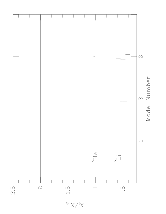
Figure 10: The solar abundance ratios for ${\vphantom{\rm Li}{}^{7}{\rm Li}}$ and ${\vphantom{\rm He}{}^{4}{\rm He}}$. The lithium abundance is dependent on both the initial abundance and on the low mass stellar yields, thus four ranges are shown for each model. The two lower ranges are for $\eta=4.5\times 10^{-10}$ and the upper ranges are for $\eta=5.5\times 10^{-10}$. Similarly the left two ranges are for the older low mass stellar yields and the right two ranges are for the newer yields. In principle the ${\vphantom{\rm He}{}^{4}{\rm He}}$ abundance also depends on our choice of initial abundance and low mass stellar yields. In practice this dependence is found to be extremely small so only one range is shown for each model. See the text for details.

shows the ratio of the predicted abundance to the observed solar abundance. Note that ${\vphantom{\rm Li}{}^{7}{\rm Li}}$ is sensitive to the choice of $\eta$, which changes the initial conditions, and the low mass stellar yields we employ. In general we find about half the solar ${\vphantom{\rm Li}{}^{7}{\rm Li}}$ can be accounted for with the yields employed here. The origin of the rest of the ${\vphantom{\rm Li}{}^{7}{\rm Li}}$ is still uncertain. Cosmic rays can only produce about 10% of the predicted ${\vphantom{\rm Li}{}^{7}{\rm Li}}$ (Vangioni-Flam et al. 1996) thus they cannot account for this deficit. This discrepancy is not too worrisome, though, since the ${\vphantom{\rm Li}{}^{7}{\rm Li}}$ yield from the $\nu$-process in type II supernovae is still uncertain by at least a factor of two.

Figure 11: The lithium as a function of iron abundance for the closed box model. All three models are quite similar, particularly on the Spite plateau. We only show the results for the older yields since the results with the newer yields are quite similar with only a slight vertical shift. The lower set of curves are for $\eta=4.5\times 10^{-10}$ and the upper set of curves are for $\eta=5.5\times 10^{-10}$. See the text for more details.

In figure 11 we show the evolution of $\log_{10}N({\rm Li})\equiv 12+\log_{10}({\rm Li/H})$ as a function of the iron abundance. The ${\vphantom{\rm Li}{}^{7}{\rm Li}}$ values with an iron abundance $[{\rm Fe/H}]\mathrel{\mathchoice{\lower 3.6pt\vbox{\halign{$\mathsurround=0pt\displaystyle\hfil#\hfil$\cr<\crcr\sim\crcr}}}{\lower 3.6pt\vbox{\halign{$\mathsurround=0pt\textstyle\hfil#\hfil$\cr<\crcr\sim\crcr}}}{\lower 3.6pt\vbox{\halign{$\mathsurround=0pt\scriptstyle\hfil#\hfil$\cr<\crcr\sim\crcr}}}{\lower 3.6pt\vbox{\halign{$\mathsurround=0pt\scriptscriptstyle\hfil#\hfil$\cr<\crcr\sim\crcr}}}}-2$ show the Spite plateau (Spite & Spite 1982) that is used to determine the primordial ${\vphantom{\rm Li}{}^{7}{\rm Li}}$ abundance. The discrepency between the primordial value and the Spite plateau is not unexpected. It either argues for a lower value for $\eta$ or for some ${\vphantom{\rm Li}{}^{7}{\rm Li}}$ depletion in stars. Many stellar models predict about a factor of two depletion of ${\vphantom{\rm Li}{}^{7}{\rm Li}}$ in stars observed on the Spite plateau (see e.g., Pinsonneault, Deliyannis, & Demarque 1992; Chaboyer & Demarque 1994; Vauclair & Charbonnel 1995). To be consistent with the higher primordial starting value, $\eta=5.5\times 10^{-10}$, requires a factor of 3–4 depletion. Such a level of depletion seems inconsistent with the observations (Lemoine et al. 1996).

The models do a good job of explaining the general trend of the data. We expect them to serve as an upper envelope to the observations with an iron abundance $[{\rm Fe/H}]\mathrel{\mathchoice{\lower 3.6pt\vbox{\halign{$\mathsurround=0pt\displaystyle\hfil#\hfil$\cr>\crcr\sim\crcr}}}{\lower 3.6pt\vbox{\halign{$\mathsurround=0pt\textstyle\hfil#\hfil$\cr>\crcr\sim\crcr}}}{\lower 3.6pt\vbox{\halign{$\mathsurround=0pt\scriptstyle\hfil#\hfil$\cr>\crcr\sim\crcr}}}{\lower 3.6pt\vbox{\halign{$\mathsurround=0pt\scriptscriptstyle\hfil#\hfil$\cr>\crcr\sim\crcr}}}}-1$ due to ${\vphantom{\rm Li}{}^{7}{\rm Li}}$ destruction in stars. The scatter in the ${\vphantom{\rm Li}{}^{7}{\rm Li}}$ abundance, particularly on the Spite plateau, is quite small. Some of the scatter is due to systematic uncertainties in the stellar atmosphere models emplyed to convert the observed line strength into an abundance. The extremely small spread predicted here shows that different evolutionary histories do not play a role in defining an intrinsic spread in the Spite plateau. If intrinsic scatter does exist in the Spite plateau it must be explained via stellar processing (see e.g., Vauclair & Charbonnel 1995) not by chemical evolution. In fact, this shows that chemical evolution does not introduce an intrinsic scatter at a level that would be difficult to extract from scatter introduced by stellar processing.

3.5 Light Elements

The chemical evolution of D and ${\vphantom{\rm He}{}^{4}{\rm He}}$ is easy; stars make ${\vphantom{\rm He}{}^{4}{\rm He}}$ and stars destroy all of their D during their pre-main sequence evolution. The chemical evolution of ${\vphantom{\rm He}{}^{3}{\rm He}}$ is more complicated. Thus we allow for two different types of ${\vphantom{\rm He}{}^{3}{\rm He}}$ evolution as previously discussed. Since D, ${\vphantom{\rm He}{}^{3}{\rm He}}$, and ${\vphantom{\rm He}{}^{4}{\rm He}}$ are all made in appreciable quantities in BBN, their abundance histories are sensitive to the choice of $\eta$ which determines their initial abundances.

3.5.1 Helium-4

The solar abundance ratio of ${\vphantom{\rm He}{}^{4}{\rm He}}$ is shown in figure 10. Since the predicted solar abundance of ${\vphantom{\rm He}{}^{4}{\rm He}}$ is insensitive to both the stellar yields and the choice of $\eta$, only one range for each model is shown in the figure. We see that there is very good agreement with the solar value, that it is largely independent of the chemical evolution model, and the scatter is extremely small. This is not surprising. BBN production provides a large initial abundance for ${\vphantom{\rm He}{}^{4}{\rm He}}$, $Y_{\rm BBN}\approx 0.24$, and is only logarithmically dependent on the choice of $\eta$ (Walker et al. 1991). The solar value of ${\vphantom{\rm He}{}^{4}{\rm He}}$, $Y_{\odot}=0.275$ (Anders & Grevesse 1989), is very close to the primordial value. Even without any production of ${\vphantom{\rm He}{}^{4}{\rm He}}$ we find a ratio $Y_{\rm BBN}/Y_{\odot}\approx 0.9$ which is well within the expected uncertainty. Any production of ${\vphantom{\rm He}{}^{4}{\rm He}}$ serves to improve this agreement. Since only a small fraction of the final ${\vphantom{\rm He}{}^{4}{\rm He}}$ is produced in stars and since all stars make ${\vphantom{\rm He}{}^{4}{\rm He}}$, we expect the scatter to be quite small as is observed.

Figure 12: The ${\vphantom{\rm He}{}^{4}{\rm He}}$ abundance as a function of the oxygen abundance. The data is from Pagel et al. (1992). Shown here are the results for the closed box model with $\eta=4.5\times 10^{-10}$ (solid line) and $\eta=5.5\times 10^{-10}$ (short-dashed line). Results for the other models are nearly identical. See the text for details.

In figure 12 we show the ${\vphantom{\rm He}{}^{4}{\rm He}}$ abundance as a function of ${\rm O/H}$. The most precise observations come from extra-galactic H ii regions. The data shown in the figure is a representative sample from Pagel et al. (1992). A more complete sample can be found in Olive & Scully (1996). As noted above we do not consider any special options for ${\vphantom{\rm N}{}^{14}{\rm N}}$ production so we will not discuss the behavior of ${\vphantom{\rm He}{}^{4}{\rm He}}$ as a function of ${\vphantom{\rm N}{}^{14}{\rm N}}$. See Fields (1996) for a thorough discussion. The fact that the initial value in these models is high compared to the data is well known and may be due to a systematic shift required in the data (Copi, Schramm, & Turner 1995a). Alternatively a model with $\eta\approx 2\times 10^{-10}$ would allow the initial value of ${\vphantom{\rm He}{}^{4}{\rm He}}$ to be in good agreement with the data as plotted. Note that a linear relation is predicted as is expected and commonly employed (Olive & Steigman 1995). The shallow slope of the line is not in good agreement with the observations. This is a standard failing of chemical evolution models. It may be due to our lack of knowledge regarding intermediate mass stars, $8<M/M_{\odot}<11$. Recall that we have interpolated between our high mass and low mass tables for these stars. If the suggestion of Woosley & Weaver (1986) that these stars return mostly ${\vphantom{\rm He}{}^{4}{\rm He}}$ to the ISM is employed the slope steepens as expected (Fields 1996).

3.5.2 Deuterium and Helium-3

       

Figure 13: The time evolution of D/H, ${\vphantom{\rm He}{}^{3}{\rm He}}$/H, and (D+${\vphantom{\rm He}{}^{3}{\rm He}}$)/H for the 3 models. The line types are as in figure 3. The data for D ($\Box$), ${\vphantom{\rm He}{}^{3}{\rm He}}$ ($\triangle$), and D+${\vphantom{\rm He}{}^{3}{\rm He}}$ ( ) are shown. The observation of D in the atmosphere of Jupiter (Niemann et al. 1996) is shown shifted slightly to the right of the pre-solar observations for clarity. The redshift scale is for a flat, $\Omega_{\rm Matter}=1$, Universe with an age of 15$\;{\rm Gyr}$. The panels represent the results for (a) models with $\eta=4.5\times 10^{-10}$ and ${\vphantom{\rm He}{}^{3}{\rm He}}$ production from Iben & Truran (1978), (b) same as (a) except we use the newer low mass stellar yields from Boothroyd & Sackmann (1996), (c) same as (a) for $\eta=5.5\times 10^{-10}$, and (d) same as (b) for $\eta=5.5\times 10^{-10}$.

The chemical evolution of D and ${\vphantom{\rm He}{}^{3}{\rm He}}$ are closely connected; D is burned to ${\vphantom{\rm He}{}^{3}{\rm He}}$ during the pre-main sequence of all stars. The time evolution of D, ${\vphantom{\rm He}{}^{3}{\rm He}}$, and ${\rm D}+{\vphantom{\rm He}{}^{3}{\rm He}}$ is shown in figure 13. The tightest constraint comes from the ISM abundance of D since it is precisely measured (Linsky et al. 1993, 1995). Note that D is not directly measured in the sun, consistent with our assumption that all D is burned to ${\vphantom{\rm He}{}^{3}{\rm He}}$ in its pre-main sequence evolution. Instead the D abundance is deduced from ${\vphantom{\rm He}{}^{3}{\rm He}}$ in the solar wind, which we assume is the ${\rm D}+{\vphantom{\rm He}{}^{3}{\rm He}}$ the sun started with (Geiss & Reeves 1972), and ${\vphantom{\rm He}{}^{3}{\rm He}}$ observed in gas rich meteorites (Black 1972). However D has been measured in the atmosphere of Jupiter via the DH/H₂ molecular abundance ratio (Niemann et al. 1996) which should also give a measure of the D in the pre-solar nebula. This value is somewhat higher than the deduced value but the uncertainties are quite large as the ratio is sensitive to chemical fractionation in the atmosphere. Helium-3 has recently been measured in the local ISM by the Ulysses satellite (Gloeckler & Geiss 1996). The high redshift D observations are from quasar absorption systems (Tytler, Fann, & Burles 1996; Burles & Tytler 1996). We note that ${\rm D}+{\vphantom{\rm He}{}^{3}{\rm He}}$ has remained roughly constant over the past 5$\;{\rm Gyr}$(Gloeckler & Geiss 1996). This has important implications for chemical evolution models (Turner et al. 1996) though the uncertainties are still too large to impose tight constraints.

The extreme production of ${\vphantom{\rm He}{}^{3}{\rm He}}$ predicted by Iben & Truran (1978) cannot be easily accommodated by any models (see figure 13a,c), unless we push the already large uncertainties on the observations to their 2- or 3-$\sigma$ values. The infall model (figure 13a,c) is the only one that approximately reproduces the ISM D observations but is only marginally in agreement with the meteoritic ${\vphantom{\rm He}{}^{3}{\rm He}}$ observation.

The models with the new low mass stellar yields do a much better job of fitting both the meteoritic and ISM ${\vphantom{\rm He}{}^{3}{\rm He}}$ observations (see figure 13b,d). In fact, since we employ extreme ${\vphantom{\rm He}{}^{3}{\rm He}}$ destruction models, it is somewhat under produced in our results. The ISM D is best fit by the closed box model (figure 13b) for $\eta=4.5\times 10^{-10}$ and by the infall model (figure 13d) for $\eta=5.5\times 10^{-10}$.

In all the models considered here there is relatively little D destruction between the time of BBN and the observations of D in quasar absorption systems at $z=3\hbox{--}4$, only about 10%. However, since the BBN production of D is very sensitive to $\eta$ (Copi, Schramm, & Turner 1995a) it is important to account for the chemical evolution when determining the primordial value of D. If we assume the observations are the primordial abundance then it is more consistent with $\eta\approx 6\times 10^{-10}$.

Figure 14: The time evolution of D/H, ${\vphantom{\rm He}{}^{3}{\rm He}}$/H, and (D+${\vphantom{\rm He}{}^{3}{\rm He}}$)/H for an outflow model with $\eta=3.2\times 10^{-10}$. See the text for details. The data is as in figure 13.

We have also considered the evolution of D and ${\vphantom{\rm He}{}^{3}{\rm He}}$ in an outflow model with $\eta=3.2\times 10^{-10}$. As is well known, chemical evolution models can be constructed from a wide range of initial abundances of D and ${\vphantom{\rm He}{}^{3}{\rm He}}$ that are consistent with the present day observations. In figure 14 we show the evolution for an outflow model where 90% of the ejecta from type II supernovae and 85% of the ejecta from type Ia supernovae escapes the region. in this model we used a 70%/30% mixture of the new and old low mass stellar yields. Furthermore we flattened the IMF to $\phi(M)\propto M^{-1.9}$ to allow for extra processing by high mass stars. Even more processing can be obtained by skewing the IMF to high mass stars at early times (Olive et al. 1996).

Finally we note that the spread in D and ${\vphantom{\rm He}{}^{3}{\rm He}}$ is predicted to be quite small. For D this is in good agreement with the observations of Linsky et al. (1993, 1995) who found nearly identical D abundances along two different lines of sight in the ISM. This lends support to our assumption that a $10^{5}M_{\odot}$ region is well mixed in the solar neighborhood. For ${\vphantom{\rm He}{}^{3}{\rm He}}$ this does not agree well with the observations in H ii regions which find a range of values, ${\vphantom{\rm He}{}^{3}{\rm He}}/{\rm H}\approx$(1–4)$\times 10^{-5}$ (Balser et al. 1994). Note, however, that the models discussed here are tuned for the solar neighborhood, not H ii regions, and thus expecting them to reproduce these results may not be reasonable. The chemical evolution model appropriate for an H ii region could be quite different than the ones employed for the solar neighborhood.

3.6 Additional Constraints

There are a number of other constraints on galactic chemical evolution models that we will discuss now. We have already used the fact that the present day gas-to-total mass fraction, $\mu=10$%–13% for all models, to fix the star formation rate so this constraint is trivially satisfied.

3.6.1 Present Day Mass Function

Figure 15: The distribution of stars, by mass, expected to currently reside in the solar neighborhood, known as the present day mass function. Only the curve for the closed box model is shown since all models are nearly identical. The data is from Scalo (1986). Since we have employed a power law IMF we do not expect to get good agreement at low masses, $\log M\mathrel{\mathchoice{\lower 3.6pt\vbox{\halign{$\mathsurround=0pt\displaystyle\hfil#\hfil$\cr<\crcr\sim\crcr}}}{\lower 3.6pt\vbox{\halign{$\mathsurround=0pt\textstyle\hfil#\hfil$\cr<\crcr\sim\crcr}}}{\lower 3.6pt\vbox{\halign{$\mathsurround=0pt\scriptstyle\hfil#\hfil$\cr<\crcr\sim\crcr}}}{\lower 3.6pt\vbox{\halign{$\mathsurround=0pt\scriptscriptstyle\hfil#\hfil$\cr<\crcr\sim\crcr}}}}0$.

The present day mass function (PDMF) is the distribution of stars by mass expected to be observed in the Universe today. Due to different lifetimes for stars of different masses, the PDMF is not the same as the IMF. Figure 15 shows a comparison of the predicted PDMF and observations from Scalo (1986). Only the curve for the closed box model is shown since all models exhibit similar behavior with minor differences at low masses, $\log M\mathrel{\mathchoice{\lower 3.6pt\vbox{\halign{$\mathsurround=0pt\displaystyle\hfil#\hfil$\cr<\crcr\sim\crcr}}}{\lower 3.6pt\vbox{\halign{$\mathsurround=0pt\textstyle\hfil#\hfil$\cr<\crcr\sim\crcr}}}{\lower 3.6pt\vbox{\halign{$\mathsurround=0pt\scriptstyle\hfil#\hfil$\cr<\crcr\sim\crcr}}}{\lower 3.6pt\vbox{\halign{$\mathsurround=0pt\scriptscriptstyle\hfil#\hfil$\cr<\crcr\sim\crcr}}}}-0.5$. The agreement with stars above solar mass, $\log M\mathrel{\mathchoice{\lower 3.6pt\vbox{\halign{$\mathsurround=0pt\displaystyle\hfil#\hfil$\cr>\crcr\sim\crcr}}}{\lower 3.6pt\vbox{\halign{$\mathsurround=0pt\textstyle\hfil#\hfil$\cr>\crcr\sim\crcr}}}{\lower 3.6pt\vbox{\halign{$\mathsurround=0pt\scriptstyle\hfil#\hfil$\cr>\crcr\sim\crcr}}}{\lower 3.6pt\vbox{\halign{$\mathsurround=0pt\scriptscriptstyle\hfil#\hfil$\cr>\crcr\sim\crcr}}}}0$, is quite good. Below this the model and observations begin to diverge. This is a common feature of a power law IMF; it cannot have curvature at low mass as required by the data. These stars do not directly contribute to the chemical evolution of the Universe since their lifetime is comparable to the age of the Universe (or larger). However, by over counting the number of low mass stars we lock some gas into these stars that could have gone into forming other, higher mass stars. Though only a small amount of the total mass is locked into these stars.

3.6.2 G Dwarf Distribution

Figure 16: The spread in the number of G-dwarf stars as a function of iron abundance. The data (heavy solid line) is from Rocha-Pinto & Maciel (1996). The line types are as in figure 3. The results for the closed box model are left out for clarity. The results for the closed box model falls between the infall and outflow models.

The iron abundance in G-dwarf stars provides a crucial and difficult, test for all chemical evolution models. The results for our models along with the data from Rocha-Pinto & Maciel (1996) are shown in figure 16. Our results are in good agreement with those in Scully et al. (1996). We only show the results for the infall and outflow models in figure 16. The scatter predicted in the G-dwarf distribution is fairly large. Though it is not sufficiently large to explain the observed distribution. The problem still remains that the models do not predict enough stars at $[{\rm Fe/H}]\sim-0.3$ and predicts too many stars at $[{\rm Fe/H}]\sim 0$. The G-dwarf distribution is intimately related to the age-metallicity relation. The model results are consistent with the fast rise in the metallicity to an almost constant value $[{\rm Fe/H}]\approx 0$ for most of the evolution. To reproduce the observed G-dwarf distribution requires slowing the rise in iron abundance.

3.6.3 Supernova Rates

The type II supernova rate for all of our models is approximately $2\times 10^{-6}$ supernovae per $10^{5}M_{\odot}$ per century. The type Ia supernova rate for all of our models is approximately $1\times 10^{-7}$ supernovae per $10^{5}M_{\odot}$ per century. If we assume the solar neighborhood is typical for the entire Galactic disk, $M_{\rm disk}=10^{11}M_{\odot}$, we predict about 2 Galactic supernovae per century. This is in good agreement with the observed Galactic supernova rate of $2.5^{+0.8}_{-0.5}$ per century (Tammann, Löffler, & Schröder 1994).

The ratio for type Ia to type II supernovae for our models is 6% for the closed box model, 12% for the infall model, and 19% for the outflow model. The expected value is about 10% (Tammann, Löffler, & Schröder 1994). The ratio is sensitive to the iron yields for both types of supernovae. The type Ia supernova rate in the outflow model is also quite sensitive to our choice of the fraction of ejected material that escapes from the region.

4 Conclusions

Three fairly standard, one zone chemical evolution models have been solved for the solar neighborhood in a stochastic manner in order to study the expected spread in abundances due to the different evolutionary histories the material could have undergone. In all cases the average behavior is in good agreement with previous work. We have studied the evolution of a $10^{5}M_{\odot}$ region for a closed box model, an infall model, and an outflow model of the solar neighborhood. A region of $10^{5}M_{\odot}$ does a very good job of explaining the observed scatter as a function of iron abundance for the heavy $\alpha$-elements, ${\vphantom{\rm O}{}^{16}{\rm O}}$, ${\vphantom{\rm Si}{}^{28}{\rm Si}}$, and ${\vphantom{\rm S}{}^{32}{\rm S}}$ (see figures 3–6). In fact, the large predicted spread for abundances at $[{\rm Fe/H}]\mathrel{\mathchoice{\lower 3.6pt\vbox{\halign{$\mathsurround=0pt\displaystyle\hfil#\hfil$\cr<\crcr\sim\crcr}}}{\lower 3.6pt\vbox{\halign{$\mathsurround=0pt\textstyle\hfil#\hfil$\cr<\crcr\sim\crcr}}}{\lower 3.6pt\vbox{\halign{$\mathsurround=0pt\scriptstyle\hfil#\hfil$\cr<\crcr\sim\crcr}}}{\lower 3.6pt\vbox{\halign{$\mathsurround=0pt\scriptscriptstyle\hfil#\hfil$\cr<\crcr\sim\crcr}}}}-2$ in the infall model may help to set limits on the amount of infall in the solar neighborhood.

In most other cases the predicted and observed spread are not in good agreement. This helps to point out where other physical processes may play an important role. The spread in the age-metallicity relation (figure 1) is not well fit by the predictions. Most of the iron in the Universe comes from type Ia supernovae in our models. We have only allowed for one type of evolutionary scenario for these supernovae. The calculations of Nomoto et al. (1996) do find a small range of iron yields for different evolutionary scenarios for supernovae. Though this alone is not sufficient to explain the spread in observations. Unlike in standard chemical evolution models, the age-metallicity relation plays an important role in constraining stochastic models. A complete understanding of stochastic chemical evolution requires an explanation of the full spread in the age-metallicity relation.

For carbon and nitrogen we also see that the predicted spread only accounts for about a half of the spread found in the data (figures 8 and 9). In this case we may be learning something about stellar evolution. In particular our assumption that the mass and initial composition are sufficient to determine all properties of a star may not be correct for low mass stars. Unlike high mass stars, the yields of low mass stars is dependent on many physical processes that are poorly understood and difficult to approximate in an accurate manner. In this work we have included yields due to extra mixing processes in stars. If this mixing is coupled to the rotational history of the star we would expect a distribution of yields for low mass stars based on a distribution of angular momenta in these stars. Such a distribution coupled with the different evolutionary histories may explain the scatter in the carbon and nitrogen abundance data.

Though we have included ${\vphantom{\rm C}{}^{13}{\rm C}}$ in our work its interpretation is much more difficult. The evolution of ${\vphantom{\rm C}{}^{13}{\rm C}}$ is strongly dependent on the cool bottom processing and mixing in low mass stars. Thus all results are very model dependent. We have found that the solar ${\vphantom{\rm C}{}^{13}{\rm C}}$ abundance and the solar ${\vphantom{\rm C}{}^{12}{\rm C}}$/${\vphantom{\rm C}{}^{13}{\rm C}}$ ratio are not well fit by any of the models (figure 7). The older yields predict that low mass stars make only about half the solar ${\vphantom{\rm C}{}^{13}{\rm C}}$ whereas the newer yields make 2–3 times the solar abundance. This is most evident for the case of the outflow model where ${\vphantom{\rm C}{}^{13}{\rm C}}$ is over produced in the new low mass stellar model. Note that it shows up strongly in the outflow model since there is so much extra processing of material. If we had included a time dependent IMF skewed towards high mass stars at early times the behavior of ${\vphantom{\rm C}{}^{13}{\rm C}}$ would not be as extreme.

From our studies we have shown that the range in baryon-to-photon ratio, $\eta\approx(3\hbox{--}5.5)\times 10^{-10}$ is consistent with the present day observations of D and ${\vphantom{\rm He}{}^{3}{\rm He}}$ for standard chemical evolution models. Of course we have only considered simple models here. Models that allow for and even larger range of $\eta$ can, and have been, constructed (see e.g., Olive et al. 1996). In general we find that the predicted spread for all the light elements is quite small. This further justifies the common use of chemical evolution to extract the primordial abundances from present day observations. Different evolutionary histories, at least for the solar neighborhood, do not introduce a significant amount of scatter and thus does not further complicate such attempts.

For ${\vphantom{\rm Li}{}^{7}{\rm Li}}$ the small spread on the Spite plateau (figure 11) argues against an intrinsic spread in the abundances due to the different histories the material could have gone through. Any intrinsic scatter would instead be due to stellar processing (Vauclair & Charbonnel 1995). Similarly, the scatter in ${\vphantom{\rm He}{}^{4}{\rm He}}$ is extremely small (figure 10). This is not surprising due to the large primordial value from BBN. Note, though, that most ${\vphantom{\rm He}{}^{4}{\rm He}}$ observations are made in extra-galactic H ii regions. Thus their evolution should not be expected to follow that of the solar neighborhood. We predict a linear relationship between ${\vphantom{\rm He}{}^{4}{\rm He}}$ and O/H as expected (figure 12). However the slope is much flatter than appears in the observations as is a common failing in chemical evolution models of the type we have considered.

Deuterium and helium-3 are the two light elements that are most strongly affected by chemical evolution. Thus chemical evolution is essential to extract their primordial abundances and test BBN. The precise observation of D in the ISM places very tight constraints on chemical evolution models. The evolution of ${\vphantom{\rm He}{}^{3}{\rm He}}$ in low mass stars also strongly affects the types of chemical evolution models we can construct to fit the observations. As we noted above, the models we consider here allow a range in the baryon-to-photon ratio, $\eta\approx(3\hbox{--}5.5)\times 10^{-10}$. Again this is due to the models we have chosen and not a general requirement. A wider range of starting values can produce satisfactory fits to the observations (Olive et al. 1996).

The spread in both of these abundances is predicted to be quite small (figure 13). For the solar neighborhood this is in good agreement with D observations along two different lines of sight in the ISM (Linsky et al. 1993, 1995). This lends some support to our assumption that regions of size $\sim 10^{5}M_{\odot}$ are well mixed in the solar neighborhood. For ${\vphantom{\rm He}{}^{3}{\rm He}}$ we would expect a larger spread based on observations in H ii regions (Balser et al. 1994) but again note that the results discussed here are tuned for the solar neighborhood. Notice that different histories do not provide an explanation for the difference in D observations in quasar absorption systems. The observed difference is approximately an order of magnitude. Though it is premature to label either, let alone both, value as primordial, it is even difficult to understand how they both can be observations of D. Starting from either value it is not known how the other value could be reproduced (Jedamzik & Fuller 1996) and why there is not a distribution of values between these two extremes.

We must again point out that observations in H ii regions and in quasar absorption systems are made in environments that can be quite different than the solar neighborhood. Thus we should not expect our models to reproduce these regions. Although the stochastic approach discussed here enjoys some success in explaining the spread of abundances in the solar neighborhood, it may be better suited for exploring quasar absorption systems and H ii regions. These regions are more consistent with lower mass gas clouds in the range $10^{5}M_{\odot}$ as employed here. Furthermore the observations of a scatter of light element abundances in these regions may indicate the need for a stochastic approach. Quasar absorption systems may be ideal for this type of approach since there are a number of different systems over a range of redshifts observed. Furthermore, metal lines have been observed in many of these systems which provides constraints on the global features of the chemical evolution model. Chemical evolution in quasar absorption systems has been studied in the standard manner (Timmes, Lauroesch, & Truran 1995; Malaney & Chaboyer 1996) and may benefit from the stochastic approach.

References

Anders, E. & Grevesse, N. 1989, Geochim. Cosmochim. Acta, 53, 197

Balser, D. S., Bania, T. M., Brockway, C. J., Rood, R. T., & Wilson, T. L. 1994, ApJ, 430, 667

Barbuy, B. & Erdelyi-Menedes, M. 1989, A&A, 214, 239

Black, D. C. 1972, Geochim. Cosmochim. Acta, 36, 347

Boesgaard, A. M. & Tripicco, M. J. 1986, ApJ, 303, 724

Boothroyd, A. I. & Malaney, R. A. 1996, ApJ, in press

Boothroyd, A. I. & Sackmann, I.-J. 1996, ApJ, in press

Boothroyd, A. I., Sackmann, I.-J., & Wasserburg, G. J. 1995, ApJ, 442, L21

Burles, S. & Tytler, D. 1996, ApJ, 460, 584

Cameron, A. G. W. & Truran, J. W. 1971, Ap&SS, 14, 179

Carbon, D. F., Barbuy, B., Kraft, R. P., Friel, E. D., & Suntzeff, N. B. 1987, PASP, 99, 335

Carswell, R. F., Rauch, M., Weymann, R. J., Cooke, A. J., & Webb, J. K. 1994, MNRAS, 268, L1

Chaboyer, B. & Demarque, P. 1994, ApJ, 433, 510

Charbonnel, C. 1994, A&A, 282, 811

 . 1995, ApJ, 453, L41

Clegg, R. E. S., Lambert, D. L., & Tomkin, J. 1981, ApJ, 250, 262

Copi, C. J., Schramm, D. N., & Turner, M. S. 1995a, Science, 267, 192

 . 1995b, ApJ, 455, L95

 . 1995c, PRL, 75, 3981

Cumming, A. & Haxton, W. C. 1996, nucl-th/9608045

Dearborn, D., Eggleton, P. P., & Schramm, D. N. 1976, ApJ, 203, 455

Denissenkov, P. A. & Weiss, A. 1996, A&A, 308, 773

Edvardsson, B., Andersen, J., Gustafsson, B., Lambert, D. L., Nissen, P. E., & Tomkin, J. 1993, A&A, 275, 101

Fields, B. D. 1996, ApJ, 456, 478

Forestini, M. & Charbonnel, C. 1996, A&A, in press

François, P. 1987, A&A, 176, 294

 . 1988, A&A, 195, 226

François, P. & Matteucci, F. 1993, A&A, 280, 136

François, P., Vangioni-Flam, E., & Audouze, J. 1990, ApJ, 361, 487

Fukazawa, Y. et al. 1996, PASJ, 48, 395

Fuller, G., Boyd, R. N., & Kallen, J. D. 1991, ApJ, 371, L11

Galli, G., Palla, F., Straniero, O., & Ferrini, F. 1994, ApJ, 432, L101

Galli, G., Stanghellini, L., Tosi, M., & Palla, Francesco 1996, astro-ph/9609184

Geiss, J. & Reeves, H. 1972, A&A, 18, 126

Gloeckler, G. & Geiss, J. 1996, Nature, 381, 210

Gratton, R. G. 1985, A&A, 148, 105

Gratton, R. G. & Ortolani, S. 1986, A&A, 169, 201

Greggio, L. & Renzini, A. 1983, A&A, 154, 279

Henning, T. & Gürtler, J. 1986, Ap&SS, 128, 199

van den Hoek, L. B. & Groenewegen, M. A. T. 1996, A&A, in press

van den Hoek, L. B. & de Jong, T. 1996, A&A, in press

Hogan, C. J. 1995, ApJ, 411, L17

Iben, I., Jr. & Truran, J. W. 1978, ApJ, 220, 980

Jedamzik, K. & Fuller, G. M. 1996, astro-ph/9609103

Laird, J. B. 1985, ApJ, 289, 556

Lemoine, M., Schramm, D. N., Truran, J. W., & Copi, C. J. 1996, ApJ, in press

Linsky, J. L., Brown, A., Gayley, K., Diplas, A., Savage, B. D., Ayres, T. R., Landsman, W., Shore, S. W., & Heap, S. 1993, ApJ, 402, 694

Linsky, J. L., Diplas, A., Wood, B. E., Brown, A., Ayres, T. R., & Savage, B. D. 1995, ApJ, 47, 353

Loewenstein, M. & Mushotzky, R. F. 1996, ApJ, 466, 695

Maeder, A. 1992, A&A, 264, 105

 . 1993, A&A, 268, 833

Magain, P. 1987, A&A, 179, 176

Malaney, R. A. & Chaboyer, B. 1996, ApJ, 462, 57

Mathews, G. J. & Schramm, D. N. 1993, ApJ, 404, 476

Matteucci, F. & Gibson, B. K. 1996, Proc. of Dark and Visible Matter in Galaxies, eds. Persic, M. & Salucci, P., ASP conf. series, in press

McWilliam, A., Preston, G. W., Sneden, C., & Searle, L. 1995, AJ, 109, 2757

Mushotzky, R. F. et al. 1996, ApJ, 456, 80

Niemann, H. B. et al. 1996, Science, 272, 846

Nomoto, K., Thielemann, F.-K., & Yokoi, Y. 1984, ApJ, 286, 644

Nomoto, K. et al. 1996, in Thermonuclear Supernovae, ed. R. Canal et al., (NATO ASI: Klumer), in press

Norris, J. E., Ryan, S. G., & Stringfellow, G. S. 1994, ApJ, 423, 386

Olive, K. A., Schramm, D. N., Scully, S. T., & Truran, J. W. 1996, astro-ph/9610039

Olive, K. A. & Scully, S. T. 1996, IJMPA, 11, 409

Olive, K. A. & Steigman, G. 1995 ApJS, 97, 490

Pagel, B. E. J., Simonson, E. A., Terlevich, R. J., & Edmunds, M. G. 1992, MNRAS, 255, 325

Pasquini, L., Liu, Q., & Pallavicini, R. 1994, A&A, 287, 191

Peterson, R. C., Kurucz, R. L., & Carney, B. W. 1990, ApJ, 350, 173

Pinsonneault, M. H., Deliyannis, C. P., & Demarque, P. 1992, ApJS, 78, 179

Rana, N. C. 1991, ARA&A, 29, 129

Renzini, A. & Voli, M. 1981, A&A, 94, 175

Rocha-Pinto, H. J. & Maciel, W. J. 1996, MNRAS, 279, 447

Rood, R. T., Bania, T. M., & Wilson, T. L. 1992, Nature, 355, 618

Rood, R. T., Bania, T. M., Wilson, T. L., & Balser, D. S. 1995, in The Light Element Abundances, Proceedings of the ESO/EIPC Workshop, ed. P. Crane, (Berlin: Springer), 201

Rugers, M. & Hogan, C. J. 1996, ApJ, 459, L1

Ryan, S. G., Norris, J. E., & Beers, T. C. 1996, ApJ, in press

Salpeter, E. E. 1955, ApJ, 121, 161

Scalo, J. M. 1986, Fund. Cosmic Phys., 11, 1

Schmidt, M. 1959, ApJ, 129, 243

 . 1963, ApJ, 137, 758

Scully, S. T., Cassé, M., Olive, K. A., & Vangioni-Flam, E. 1996, astro-ph/9607106

Shields, G. A. 1990, ARA&A, 28, 525

Songaila, A., Cowie, L. L., Hogan, C. J., & Rugers, M. 1994, Nature, 368, 599

Spite, F. & Spite, M. 1982, A&A, 115, 357

Steigman, G. & Tosi, M. 1995, ApJ, 453, L173

Talbot, R. J. & Arnett, W. D. 1971, ApJ, 170, 409

Tammann, G. A., Löffler, W., Schröder, A. 1994, ApJS, 92, 487

Thorburn, J. A. 1994, ApJ, 421, 318

Timmes, F. X., Lauroesch, J. T., & Truran, J. W. 1995, ApJ, 451, 468

Timmes, F. X., Woosley, S. E., & Weaver, T. A. 1995, ApJS, 98, 617 (TWW)

Tinsley, B. 1972, A&A, 20, 383

 . 1980, Fund. Cosmic, Phys., 5, 287

Tomkin, J., Sneden, C., & Lambert, D. L. 1986, ApJ, 302, 415

Tosi, M. 1988, A&A, 197, 33

Turner, M. S., Truran, J. W., Schramm, D. N., & Copi, C. J. 1996, ApJ, 466, L59

Tytler, D., Fann, X.-M., Burles, S. 1996, Nature, 381, 207

Vangioni-Flam, E., Cassé, M., Fields, B. D., & Olive, K. A. 1996, ApJ, 468, 199

Vauclair, S. & Charbonnel, C. 1995, A&A, 295, 715

Walker, T. P., Steigman, G., Schramm, D. N., Olive, K. A., & Fields, B. D. 1993, ApJ, 413, 562

Walker, T. P., Steigman, G., Schramm, D. N., Olive, K. A., & Kang, H. 1991, ApJ, 376, 51

Wasserburg, G. J., Boothroyd, A. I., & Sackmann, I.-J. 1995, ApJ, 447, L37

Weiss, A., Wagenhuber, J., & Denissenkov, P. A. 1996, astro-ph/9512120

Wielen, R., Fuchs, B., & Dettbarn, C. 1996, A&A, in press

Woosley, S. E., Langer, N., & Weaver, T. A. 1993, ApJ, 411, 823

 . 1995, ApJ, 448, 315

Woosley, S. E. & Weaver, T. A. 1986, ARA&A, 24, 205

 . 1995, ApJS, 101, 181