Measurement of Galaxy Distances

Abstract

Six of the principal galaxy distance indicators are discussed: Cepheid variables, the Tully-Fisher relation, the $D_{n}$-$\sigma$ relation, Surface Brightness Fluctuations, Brightest Cluster Galaxies, and Type Ia Supernovae. The role they play in peculiar velocity surveys and Hubble constant determination is emphasized. Past, present, and future efforts at constructing catalogs of redshift-independent distances are described. The chapter concludes with a qualitative overview of Malmquist and related biases.

To appear in “Formation of Structure in the Universe,”

A. Dekel and J. Ostriker, Eds. (Cambridge University Press)

1 Introduction

The measurement of galaxy distances is one of the most fundamental problems in astronomy. To begin with, we would simply like to know the scale of the cosmos; we do so by determining the distances to galaxies. Beyond this, galaxy distances are the key to measuring the Hubble constant $H_{0},$ perhaps the most important piece of information for testing the validity of the Big Bang model. Finally, galaxy distances are necessary if we are to study the large-scale peculiar velocity field. Peculiar velocity analysis is among the most promising techniques for confirming the gravitational instability paradigm for the origin of large-scale structure, deducing the relative distributions of luminous and dark matter, and constraining the value of the cosmological density parameter $\Omega_{0}.$ In this Chapter, I will describe a number of the methods used for measuring galaxy distances, and discuss their application to the $H_{0}$ and peculiar velocity problems. When appropriate, I will comment on their relevance to determination of other cosmological parameters as well. The goal of this Chapter is not to present an exhaustive review of galaxy distance measurements, but rather to provide a summary of where matters stand, and an indication of what the next few years may bring.

1.1 Peculiar Velocities versus $H_{0}$

What it means to “measure a galaxy’s distance” depends on whether one is interested in studying peculiar velocities or determining the value of the Hubble constant. A galaxy’s peculiar velocity may be estimated given its “distance” in km s^-1—the part of its radial velocity due solely to the Hubble expansion. The same object provides an estimate of $H_{0}$ only if one can measure its distance in metric units such as megaparsecs. What this means in practice is that accurate peculiar velocity studies may be carried out today, despite the fact that $H_{0}$ remains undetermined at the $\sim\,$20% level.

Another basic distinction between velocity analysis and the search for $H_{0}$ concerns the distance regimes in which they are optimally conducted. Peculiar velocity surveys are best carried out in the “nearby” universe, where peculiar velocity errors are comparable to or less than the peculiar velocities themselves. The characteristic amplitude of the radial peculiar velocity, $v_{p},$ is a few hundred km s^-1 at all distances, whereas the errors we make in estimating $v_{p}$ grow linearly with distance (§3). It turns out that the “break-even” point occurs at distances of $\sim\,$5000 km s^-1. Although we may hope to glean some important information (such as bulk flow amplitudes) on larger scales, our ability to construct an accurate picture of the velocity field is restricted to the region within about 50$h^{-1}$ Mpc. In the Hubble constant problem, by contrast, peculiar velocities are basically a nuisance. We would like them to be a small fraction of the expansion velocity, so that we incur as small as possible an error by neglecting them. This is best achieved by using comparatively distant objects, $d\lower 2.15277pt\hbox{$\,\buildrel>\over{\sim}\,$}\ 7000\ {\rm km}\,{\rm s}^{-1},$ as tracers of the expansion.

On the other hand, to obtain the absolute distances needed to measure $H_{0},$ we must first calibrate our distance indicators locally ($\lower 2.15277pt\hbox{$\,\buildrel<\over{\sim}\,$}2000\ {\rm km}\,{\rm s}^{-1}$). This is because the distance indicators capable of reaching the “far field” ($\lower 2.15277pt\hbox{$\,\buildrel>\over{\sim}\,$}7000\ {\rm km}\,{\rm s}^{-1}$) of the Hubble flow generally have no a priori absolute calibration (cf. §1.2). The only reliable distance indicator that can bridge the gap between the Milky Way and the handful of Local Group galaxies whose absolute distances are well-known, and galaxies beyond a few Mpc, is the Cepheid variable method (§2), which is limited to distances $\lower 2.15277pt\hbox{$\,\buildrel<\over{\sim}\,$}2000\ {\rm km}\,{\rm s}^{-1}.$ As a result, Hubble constant measurement is inherently a two-step process: local calibration in galaxies with Cepheid distances, followed by distance measurements in the far field where the effect of peculiar velocities is small. The local calibration step is unnecessary in peculiar velocity studies.

Although peculiar velocity surveys and $H_{0}$ measurement differ in the ways just discussed, the two problems are, ultimately, closely related. Many distance indicator methods have been and are being used for both purposes. Indeed, a distance indicator calibrated in km s^-1 may be turned into a tool for measuring $H_{0}$ simply by knowing the distances in Mpc to a few well-studied objects to which it has been applied. This Chapter will thus be organized not around the peculiar velocity-$H_{0}$ distinction, but rather around methods of distance estimation.

1.2 Distance Indicators

Measuring the distance to a galaxy almost always involves one of the following properties of the propagation of light: (1) The apparent brightness of a source falls of inversely with the square of its distance; (2) The angular size of a source falls off inversely with its distance. As a result, we can determine the distance to an object by knowing its intrinsic luminosity or linear size, and then comparing with its apparent brightness or angular size, respectively. If all objects of a given class had approximately the same absolute magnitude, we could immediately determine their distances simply by comparing with their apparent magnitudes. Such objects are called standard candles. Similarly, classes of objects whose intrinsic linear sizes are all about the same are known as “standard rulers.” True standard candles or rulers are, however, extremely rare in astronomy. It is much more often the case that the objects in question possess another, distance-independent property from which we infer their absolute magnitudes or diameters. For example, the rotation velocities of spirals galaxies are good predictors of their luminosities (§3), while the central velocity dispersions and surface brightnesses of ellipticals together are good predictors of their diameters (§4). Whether standard candles or rulers, or members of the more common second category, objects whose absolute magnitudes or diameters we can somehow ascertain are known as Distance Indicators, or DIs.

Absolute calibration of most DIs is not straightforward. One discovers that a particular distance-independent property is a good predictor of absolute magnitude because it is well correlated with the apparent magnitudes of objects lying at a common distance—in a rich cluster of galaxies, for example. Such data may be used to determine the mathematical form of the correlation (e.g., linear with a given slope). However, the cluster distance in most cases is not accurately known. Thus, the predicted absolute magnitude corresponding to a given value of the distance-independent property—the “zero point” of the DI—remains undetermined up to a constant, assuming one has no rigorous, a priori physical theory of the correlation, as is usually the case (but see below). Any distances obtained from the DI at this point will be in error by a fixed scale factor. This situation is obviously unacceptable for the Hubble constant problem, in which absolute distances are required. The remedy is to determine the zero point of the DI by applying it to galaxies whose true distances have been determined by an independent technique (e.g., Cepheid variables), as discussed above. Such a DI is said to be “empirically” calibrated.

For peculiar velocity surveys, the situation is simpler because absolute calibration is not required. However, the DI must still be calibrated such that it yields distances in km s^-1, the radial velocity due to Hubble flow. For this, one must apply the DI to many galaxies, widely enough distributed around the sky and at large enough distances that peculiar velocities tend to cancel out. Only then can redshift be taken as a good indicator on average of distance in km s^-1, and a calibration in velocity units thereby obtained (Willick et al. 1995, 1996). Empirical DI calibration, in this sense, is needed even for peculiar velocity work.

DIs of this sort tend to make some people nervous. They argue that a good distance estimation method should be based on solid, calculable physics. There are, in fact, a few such techniques. One involves exploitation of the Sunyaev-Zeldovich effect in clusters, in which comparison of Cosmic Microwave Background distortions and the X-ray emission produced by hot, intracluster gas yields the physical size of the cluster (cf. Rephaeli 1995 for a comprehensive review). Another method involves modeling time delays between multiple images of gravitationally lensed background objects (see the Chapter by Narayan and Bartelmann in this volume). Other DIs for which theoretical absolute calibration may be possible are Type II Supernovae, whose expansion velocities may be related to luminosities (Montes & Wagoner 1995; Eastman, Schmidt, & Kirshner 1996), and Type Ia Supernovae, whose luminosities may be calculated from theoretical modeling of the explosion mechanism (Fisher, Branch, & Nugent 1993). Such approaches are indeed promising, and will undoubtedly contribute to the measurement of $H_{0}$ over the next decade. However, at present these methods should be considered preliminary. Some of the underlying physics remains to be worked out, and many of the underlying assumptions will need to be tested. Furthermore, the data needed to implement such techniques are currently rather scarce. With the exception of Type Ia Supernovae (discussed in §6 in their traditional, empirical context), I will not discuss these methods further in this Chapter.

I will focus instead on methods that require empirical calibration. These DIs arise from astrophysical correlations Nature was kind enough to provide us with, but mischievous enough to deny us a full understanding of. The canonical wisdom, which states that we need hard physical theory that explains a DI in order to trust it, is a bit too exacting given our present theoretical and observational capabilities. We should conditionally trust our empirical DIs while recognizing the uncertainties involved. In particular, we must remember that since they possess no a priori absolute calibration, they must (for measuring $H_{0}$) be carefully calibrated locally. We must also remain open to the possibility that they may not behave identically in different environments and at different redshifts. Our belief in their utility should be tempered by a healthy skepticism about their universality, and the distance estimates we make with them subjected to continuing consistency checks.

2 Cepheid Variables

Cepheids variable stars have been fundamental to unlocking the cosmological distance scale since Henrietta Leavitt used them in 1912 to estimate the distances to the Magellanic Clouds. Of the various DIs discussed in this Chapter, the Cepheid method is the only one involved in the Hubble constant but not the peculiar velocity problem. Indeed, it is probably safe to say that the raison d’être for Cepheid observations is the ultimate determination of $H_{0}.$ They will do so, however, in conjunction with, not independently of, the secondary distance indicators discussed in later sections.

Cepheids are post-main sequence stars that occupy the instability strip in the H-R diagram. They pulsate according to a characteristic “sawtooth” pattern, with periods that can range from a few days to a good fraction of a year. Cepheids exhibit an excellent correlation between mean luminosity (averaged over a pulsation cycle) and pulsation period. This correlation is shown in Figure 1 for Cepheids recently measured by the Hubble Space Telescope (HST) in the nearby galaxy M101 (solid points), and also for Cepheids in the Large Magellanic Cloud (LMC) as they would appear if the LMC lay at the distance of M101. It is apparent that the correlation is extremely similar for the two galaxies. Modern calibrations of the Cepheid Period-Luminosity (P-L) relation in the $V$ and $I$ bandpasses are

$$M_{V}=-2.76\left[\log(P)-1.0\right]-4.16$$ (1)

and

$$M_{I}=-3.06\left[\log(P)-1.0\right]-4.87$$ (2)

(Ferrarese et al. 1996). The absolute zero points of these P-L relations have been obtained by observing Cepheids in the the Large and Small Magellanic Clouds, whose distances are known from main sequence fitting (Kennicut, Freedman, & Mould 1995). Equations (1) and (2) show that Cepheid variables are intrinsically bright stars. Even short-period ($P\simeq 10^{d}$) Cepheids have absolute magnitudes $M_{V}<-4,$ and long-period ($P\simeq 50$–$100^{d}$) Cepheids are 2–3 magnitudes brighter still. It follows that individual Cepheid stars can be observed at relatively large distances. Indeed, with the HST Cepheids can be observed out to the distance of the Virgo cluster and possibly beyond. To be useful as distance indicators, however, Cepheids cannot be merely detected. Because they are found in crowded fields, they must be well above the limit of detectability at all phases in order to be accurately photometered. These stringent requirements place a limit of $m_{V}\simeq 26$ mag, much brighter than the HST detection limit of $\sim\,$30 mag, for distance scale work using Cepheids.

Figure 1: Cepheid variable Period-Luminosity (PL) relations for the $V$ and $I$ bandpasses. Data for M101 and the Large Magellanic Cloud are shown. Adapted from Ferrarese et al. (1996).

Cepheids yield distances to their host galaxies by comparison of their absolute magnitudes, inferred from the P-L relation, with their observed apparent magnitudes. Specifically, the distance to the host galaxy is obtained by fitting equations (1) and (2), plus a distance modulus offset $\mu=5\log(d/10)$ (where $d$ is in parsecs), to the observed $m_{V}$ and $m_{I}$ versus $\log(P)$ diagram. (The same exercise may of course be carried out in other bandpasses as well.) An important advance has been made in recent years by Freedman, Madore, and coworkers, who have developed a method for correcting for extinction in the host galaxies (Freedman & Madore 1990; Freedman, Wilson, & Madore 1991). In brief, the photometry is done in several bandpasses, and the magnitudes corrected for an assumed value of the extinction within the host galaxy. The distance modulus is determined for each bandpass, as described above. The value of extinction which brings the distance moduli in the various bands into agreement is assumed to be the correct one. This technique works best when data for a wide range of wavelengths, including if possible the near infrared, are available.

The great utility of Cepheids has been recognized in the designation of an HST Key Project to measure Cepheid distances for 20 nearby galaxies. This program, led by Wendy Freedman, Robert Kennicut, and Jeremy Mould, produced its first results in late 1994. As of this writing (July 1996), Cepheid distances from the Key Project are available for only a handful of galaxies. Distances for the remaining galaxies are expected to become available over the next few years. The results that have received the greatest attention to date involve the Virgo cluster galaxy M100, in which over 50 Cepheid variables have now been accurately measured (Freedman et al. 1994; Mould et al. 1995; Ferrarese et al. 1996). Fitting the universal P-L relations above to the M100 data yields a distance of $16.1\pm 1.3$ Mpc. When combined with a suite of assumptions concerning the morphology and peculiar velocity of the Virgo cluster, this distance suggests a Hubble constant of about 85 km s${}^{-1}\,$Mpc^-1(Freedman et al. 1994).

Unfortunately, the Hubble constant estimate obtained from M100 has received undue attention. This is understandable, given that determination of $H_{0}$ is the long-term aim of the Key Project. And, of course, values of $H_{0}$ in excess of $\sim\,$75 km s${}^{-1}\,$Mpc^-1 are difficult to square with most estimates of the age of the universe based on its oldest constituents. But as the Key Project group has emphasized (Kennicutt, Freedman, & Mould 1995), a single galaxy in the Virgo cluster with a good Cepheid distance does not allow one to estimate the Hubble constant with any accuracy. In fact, the Virgo cluster is a poor laboratory in which to estimate $H_{0}$ no matter how many galaxies one has Cepheid distances for. The reasons are simple: Virgo’s depth is a good fraction ($\sim\,$30%) of its distance, and its peculiar velocity is likely to be a good fraction ($\sim\,$20–30%) of its Hubble velocity. The velocity/distance ratio of any single Virgo object, or even group of objects, may therefore be a poor approximation of $H_{0},$ and it is difficult to gauge the systematic errors that affect it.

Thus, Cepheid variables will not themselves be used to measure $H_{0}.$ Instead, they will be used to obtain accurate distances for several tens of galaxies within about 20$h^{-1}$ Mpc. These galaxies will in turn serve as calibrators for the secondary distance indicators, such as Type 1a Supernovae and the Tully-Fisher relation, that are applicable in the far field of the Hubble flow (and occupy the remainder of this Chapter). Initial steps in this direction have already been taken by Sandage, Tammann, and coworkers (Sandage et al. 1996), who used HST Cepheid distances (their own, not those of the Key Project) to calibrate historical and contemporary Type Ia Supernovae. When they apply this calibration to distant Type Ia SNe (Tammann & Sandage 1995), they derive $H_{0}=56$–58 km s${}^{-1}\,$Mpc^-1 (the lower value applies to $B$-band, and the higher value to $V$-band, measurements; Sandage et al. 1996). There is considerable controversy, however, surrounding the calibration of the historical photometry used in the SNe Ia calibration. Furthermore, the Sandage group has neglected the correlation between the peak luminosity of SNe Ias and the width of their light curves, an effect which now appears important (§6). Until these issues are resolved, and agreement between the Sandage and HST Key Project groups on local Cepheid distances achieved, estimates of $H_{0}$ based on this approach should be considered preliminary.

3 The Tully-Fisher Relation for Spiral Galaxies

It has been stated that the Tully-Fisher (TF) relation is the “workhorse” of peculiar velocity surveys. One can anticipate a time in the not so distant future when more accurate techniques may supplant it, but for the next few years at least, the TF relation is likely to remain the most widely used distance indicator in cosmic velocity studies. Its role in such studies to date has been, in fact, too large to be reviewed here, and interested readers are referred to Strauss & Willick (1995), §7. Several recent developments are discussed in §8 below.

The TF relation is one of the most fundamental properties of spiral galaxies. It is the empirical statement of an approximately power-law relation between luminosity and rotation velocity. Specifically, it is found that

$$L\propto v_{{\rm rot}}^{\alpha}\,,$$ (3)

or, using the logarithmic formulation preferred by working astronomers,

$$M=A-b\eta\,.$$ (4)

In equation (4) $M=-2.5\log(L)+{\rm const.}$ is the absolute magnitude, and the velocity width parameter $\eta\equiv\log(2v_{{\rm rot}})-2.5,$ where $v_{{\rm rot}}$ is expressed in km s^-1, is a useful dimensionless measure of rotation velocity.

Figure 2: TF relations in four bandpasses. The absolute magnitudes are given in units such that $d=10^{0.2(m-M)}$ is the galaxy distance in km s^-1. Adapted from Strauss & Willick (1995).

An important fact, not always sufficiently appreciated, is that the power law exponent $\alpha$ does not have a unique value. The details of both the photometric and spectroscopic measurements affect it. A typical result found in contemporary studies is $\alpha\simeq 3.$ The corresponding value of the “TF slope,” $b,$ is $\sim 7.5.$ However, slight changes in the details of measurement can result in significant changes in $b.$ This is illustrated in Figure 2, in which TF relations in four bandpasses are plotted. The optical bandpasses ($B,$ $R,$ and $I$) all represent data from the sample of Mathewson et al. (1992). In each case the slope is $<7.$ This is because Mathewson et al. defined their velocity widths rather differently than most observers, with the result that small velocity widths are made smaller still relative to other width measurement systems, while large velocity widths are unchanged in comparison with other systems. If one were to transform the Mathewson et al. widths to those of standard systems, one would obtain and $I$-band TF slope of $\sim 7.7,$ comparable to other $I$-band samples (Willick et al. 1997). Note, however, that the slope increases steadily from $B$ to $I.$ This reflects a general trend of increasing TF slope toward larger wavelengths, which was noted over a decade ago (Bottinelli et al. 1983). The $H$-band data come from the compilation of Aaronson et al. (1982), as reanalyzed by Tormen & Burstein (1995) and Willick et al. (1996). The $H$-band TF slope is considerably greater than its optical counterparts. In part this reflects the trend just noted. However, to a greater extent it is due to the relatively small apertures within which the $H$-band photometry is done: the TF slope increases as the photometric aperture size is decreased (Willick 1991). Infrared TF samples in which total magnitudes were measured exhibit TF slopes not much in excess of the optical values (Bernstein et al. 1994).

The numerical value of the TF zero point $A$ has no absolute significance in itself, reflecting mainly the photometric system in which the TF measurements are done. Absolute magnitudes measured in different bandpasses can differ numerically by a few magnitudes for a given object. Clearly, this must have no meaning for distance measurements, and it is the zero point that absorbs such differences. For any given measurement system, however, the value of $A$ is highly significant. To see this, consider how the TF relation is used to infer distances and peculiar velocities. Given a measured apparent magnitude $m$ and width parameter $\eta,$ one infers the distance modulus to the galaxy as $\mu=m-(A-b\eta).$ The corresponding distance $d\propto 10^{0.2\mu}.$ It follows that an error $\delta\!A$ in the TF zero point thus corresponds to a fractional distance error $f=10^{-0.2\delta\!A}.$ A Hubble constant inferred from such distances will then be off by a factor $f^{-1}.$ For peculiar velocities, calibration of the TF relation consists in choosing $A$ such that $d\equiv 10^{0.2[m-(A-b\eta)]}$ gives a galaxy’s distance in km s^-1. There is no requirement that it yield the distance in Mpc. Nonetheless, as mentioned above, zero point calibration errors are still possible. Errors in $A$ produce distances in km s^-1 that differ by a fraction $f$ from the true Hubble velocity, with resultant peculiar velocity errors $\delta v_{p}=-fd.$

The TF relation has a rich history (cf. Bottinelli et al. 1983) which can not be discussed in any detail here. Its discovery is generally credited to Tully & Fisher (1977), who were the first to suggest a linear correlation between absolute magnitude and log rotation speed. Until the late 1980s, the velocity widths used in TF studies were generally obtained from analysis of the 21 cm line profiles, rather than from direct measurements of rotation curves. Thus, the TF relation was (and to some extent remains) closely associated with 21 cm radio astronomy. There is no inherent connection, however, between the TF relation and the 21 cm line. The TF relation is also closely associated in the minds of many with infrared magnitudes. This is largely due to the pioneering $H$-band ($1.6\,\mu$m) TF work of a group headed by the late Marc Aaronson in the late 1970s through the mid-1980s (e.g., Aaronson et al. 1980, 1982, 1986). This group argued that the infrared was better than the optical for TF purposes because infrared magnitudes are less subject to internal and Galactic extinction (§3.2), and because they are sensitive mainly to the old stellar population that best traces mass. While these arguments are true at some level, work over the last decade has demonstrated that CCD imaging photometry in red passbands (e.g., $R$ or $I$) results in TF relations that, empirically, work as well or better than the $H$-band version (Pierce & Tully 1988, 1992; Willick 1991; Han 1992; Courteau 1992; Bernstein 1994; Willick et al. 1995,1996).

3.1 The TF Relation and Galaxy Structure

Many workers have attempted to “explain” the TF relation on the basis of physical principles and models of galaxy formation. While these attempts can claim some modest successes, it is probably fair to say that a true explication of the TF relation remains elusive. One can argue heuristically that something like the TF relation must exist: Assuming that luminosity is proportional to mass, and that a virial relation $v^{2}\sim GM/R$ holds for spirals, it follows that $L\propto M\propto Rv^{2}.$ If one further notes that spirals have characteristic surface brightnesses $I\propto L/R^{2}$ that varies little from galaxy to galaxy, then $R\propto L^{\frac{1}{2}},$ and it follows that $L\propto v^{4}.$ This was indeed the power-law exponent (i.e., $b\simeq 10$) originally found by the Aaronson group, and the argument seemed reasonable to them (Aaronson, Huchra, & Mould 1979).

However, quite a few loose ends remain. First, as noted above, contemporary measures of the TF slope suggest that the exponent is closer to 3 than to 4. The aperture and wavelength dependences noted above tell us that the TF slope is not determined strictly by idealized dynamics, but depends also on the details of the distribution—in both space and wavelength—of the starlight emitted by the galaxy. Furthermore, while a number of theoretical approaches can approximately predict the TF slope, no realistic model has successfully accounted for its rather small ($\sim\,$0.3 mag; see below) intrinsic scatter (Eisenstein & Loeb 1996).

Another, more fundamental, problem is that the TF relation is evidently connected with the phenomenon of flat rotation curves (RCs) exhibited by most spiral galaxies. Were the RCs not flat, there would be no well-defined rotation velocity, and one would expect the TF relation to require a very specific type of velocity width measurement. In fact, a well-defined TF relation is found regardless of the specific algorithm for measuring rotation velocity (although slight variations of slope and zero point arise as a result of algorithmic differences). Whether one measures HI profile widths, asymptotic rotation velocities, “isophotal” rotation velocities (Schlegel 1996), or maximum rotation velocities, basically similar TF relations result. Because the origin of flat rotation curves is connected with the nature of dark matter, it follows that we cannot fully understand the TF relation until we understand how galaxies form in their dark matter halos.

3.2 Applying the TF Relation: A Few Details

Widely appreciated by practitioners of the TF relation, but often hidden to the wider astronomical public, are the careful correction procedures applied to the magnitudes and velocity widths that go into the TF relation. Probably the most important step is correction for projection of the disk on the plane of the sky. The observed velocity width is smaller by a factor $\sin(i),$ where $i$ is the galaxy inclination, than the intrinsic value. Observers correct for this by esimating $i$ from the apparent ellipticity of the galaxy disk. Modern CCD observations allow one to fit elliptical isophotes to the galaxy image; these isophotes typically converge to a constant ellipticity $\varepsilon$ in the outer regions. When CCD surface photometry is not available (as is the case for many of the older infrared data), one simply takes $\varepsilon=1-b/a,$ where $a$ and $b$ are the major and minor axis diameters of the galaxy obtained from photographic data. Whichever method is used, the inclination $i$ is taken to be a function of $\varepsilon.$ A typical formula employed is

$$\cos^{2}i=\left\{\begin{array}[]{ll}\frac{(1-\varepsilon)^{2}-(1-\varepsilon_{max})^{2}}{1-(1-\varepsilon_{max})^{2}}\,,&\varepsilon<\varepsilon_{max}\,;\\ 0\,,&\varepsilon\geq\varepsilon_{max}\,,\end{array}\right.$$ (5)

where $\varepsilon_{max}\simeq 0.8$ is the ellipticity exhibited by an edge-on spiral. It is apparent that formulae such as equation (5) are at best approximations, hopefully valid in a statistical sense. However, they are usually the best we can do, and are certainly far better than doing nothing. Still, the inclination correction to the widths can go seriously awry at small inclinations, and most TF samples exclude galaxies with $i\lower 2.15277pt\hbox{$\,\buildrel<\over{\sim}\,$}40^{\circ}.$

Another tricky detail of the TF relation is correcting for internal extinction. As a spiral galaxy tilts toward edge-on orientation, it becomes fainter. Since spirals are viewed at a range of orientations, it is important to correct for this effect. The most widely used correction is to brighten the raw magnitudes by an amount $C_{{\rm int}}\times\log(a/b),$ where $C_{{\rm int}}$ is the internal extinction coefficient. Studies have shown that $C_{{\rm int}}$ is bandpass-dependent, as one might expect. However, in the optical red ($R$ and $I$ bandpasses), the wavelength-dependence is very weak, and $C_{{\rm int}}\simeq 1$ is a good approximation (Burstein, Willick, & Courteau 1995; Willick et al. 1996,1997). A controversial question is whether internal extinction depends on any galaxian property other than axial ratio. Giovanelli et al. (1995) argued that it is luminosity-dependent, but Willick et al. (1996) reached the opposite conclusion through a TF-residual analysis. This issue merits further consideration in the future.

3.3 The TF Scatter

Of great importance to applications of the TF relation is its scatter $\sigma_{{\rm TF}},$ the rms magnitude dispersion about the mean relation $M(\eta).$ This scatter is composed of three basic contributions: magnitude and velocity width measurement errors, and intrinsic or “cosmic” scatter. Of the three, recent analyses have suggested that the second and third are about equally important, contributing $\sim 0.25$–$0.30$ mag each (Willick et al. 1996). Photometric measurement errors are quite small in comparison. Thus, the overall TF scatter is about 0.4 mag. It is significant that $\sigma_{{\rm TF}}$ determines not only random distance errors ($\frac{\delta d}{d}\simeq 0.46\,\sigma_{{\rm TF}}$), but also systematic errors associated with statistical bias effects (§9). Knowing $\sigma_{{\rm TF}}$ is therefore crucial for assessing the reliability of TF studies. (An analogous statement applies to the scatter of the other DIs discussed in this Chapter as well.)

I would be remiss if I did not mention that the TF scatter remains controversial. Estimates of $\sigma_{{\rm TF}}$ have varied widely in the last decade. Bothun & Mould (1987) suggested that $\sigma_{{\rm TF}}$ could be made as small as $\lower 2.15277pt\hbox{$\,\buildrel<\over{\sim}\,$}0.25$ mag with a velocity width-dependent choice of photometric aperture. Pierce & Tully (1988) also found $\sigma_{{\rm TF}}\simeq 0.25$ using CCD data in the Virgo and Ursa Major clusters. Willick (1991) and Courteau (1992) found somewhat higher but still small values of the TF scatter ($\sigma_{{\rm TF}}=0.30$–0.35 mag). Bernstein et al. (1994) found the astonishing value of 0.1 mag for the Coma Cluster TF relation using $I$-band CCD magnitudes and carefully measured HI velocity widths.

Unfortunately, these relatively low values have not been borne out by later studies using more complete samples. Willick et al. (1995,1996,1997) calibrated TF relations for six separate samples comprising nearly 3000 spiral galaxies, and found typical values of $\sigma_{{\rm TF}}\simeq 0.4$ mag for the CCD samples. Willick et al. (1996) argued that the large sample size and a relatively conservative approach to excluding outliers drove up earlier, optimistically low estimates of the TF scatter. Other workers, notably Sandage and collaborators (e.g., Sandage 1994; Federspiel et al. 1994) have taken an even more pessimistic view of the accuracy of the TF relation, suggesting that typical spirals scatter about the TF expectation by 0.6–0.7 mag.

How can one reconcile this wide range of values? At least part of the answer lies in different workers’ preconceptions and preferences. Those excited at the possiblity of finding a more accurate way of estimating distances tend to find low ($\sigma_{{\rm TF}}\lower 2.15277pt\hbox{$\,\buildrel<\over{\sim}\,$}0.3$ mag) values. Those who doubt the credibility of TF distances tend to find high ($\sigma_{{\rm TF}}\lower 2.15277pt\hbox{$\,\buildrel>\over{\sim}\,$}0.5$ mag) ones. It is possible to arrive at such discrepant results in part because the samples differ so dramatically. Perhaps it is only justified to speak of a particular value of the TF scatter for a given set of sample selection criteria; hopefully, this issue will be clarified in the years to come.

There is one galaxian property with which the TF scatter demonstrably appears to vary, however, and that is luminosity (velocity width). Brighter galaxies exhibit a smaller TF scatter than fainter ones (Federspiel et al. 1994; Freudling et al. 1995; Willick et al. 1997). Part of this effect is undoubtedly due to the fact that the errors in $\eta=\log\Delta v-2.5$ go as $(\Delta v)^{-1},$ if errors in $\Delta v$ itself are roughly constant as is most likely the case. Such velocity width errors translate directly into a TF scatter that increases with decreasing luminosity. A careful study of whether the intrinsic TF scatter varies with luminosity has not yet been carried out.

3.4 Future Directions

An intriguing recent development been application of the TF relation to relatively high-redshift galaxies. This has been made possible by the advent of large-aperture telescopes capable of measuring rotation curves out to redshifts of $z\simeq 1.$ Vogt et al. (1996) measured rotation curves and magnitudes for nine field galaxies in the redshift range $0.1\lower 2.15277pt\hbox{$\,\buildrel<\over{\sim}\,$}z\lower 2.15277pt\hbox{$\,\buildrel<\over{\sim}\,$}1$ using the Keck 10-meter telescope. They found such objects obey a TF relation similar to that of local objects, with only a modest shift ($\Delta M_{B}\lower 2.15277pt\hbox{$\,\buildrel<\over{\sim}\,$}0.6$ mag) toward brighter magnitudes. This is illustrated in Figure 3, in which the Vogt et al. data are plotted along with the TF relation derived by Pierce & Tully (1992). However, a very different conclusion has been reached by Rix et al. (1996), who combined photometry with fiber-optic spectroscopy of spirals at moderate ($z\simeq 0.25$) redshift. Rix et al. conclude that even at such modest look-back times, spiral galaxies are significantly ($\sim 1.5$ mag) brighter than their local counterparts. If the TF relation is to be applied to problems such as peculiar velocities at high redshift or estimation of $q_{0},$ its evolution with redshift will have to be understood. This is an observatonal problem which deserves, and will undoubtedly receive, considerably more attention in the near future.

Figure 3: Rotation velocity versus absolute magnitude for spiral galaxies at a median redshift of $\sim\,$0.5. This figure has been adapted from Vogt et al. (1996).

4 The $D_{n}$-$\sigma$ and Fundamental Plane Relations for Elliptical Galaxies

If the TF relation has been the workhorse of modern velocity field studies, the $D_{n}$-$\sigma$ relation has been a short step behind. The closest analogue to the TF relation for elliptical galaxies is actually the predecessor of $D_{n}$-$\sigma$, the Faber-Jackson (FJ) relation. FJ expresses the power-law correlation between an elliptical galaxy’s luminosity and its internal velocity dispersion,

$$L\propto\sigma_{e}^{\alpha}\,,$$ (6)

where the exponent $\alpha$ was found empirically to be $\sim 4\pm 1$ (Faber & Jackson 1976; Schechter 1980; Tonry & Davis 1981). Although discovered around the same time, and viewed as closely related in physical origin, TF and FJ were not considered equivalently good distance indicators. It was clear from the outset that the scatter in the FJ relation was about twice that of the TF relation, on the order of 0.8 mag. Thus, while the TF relation flourished in the early 1980s as a tool of distance measurement (§3), elliptical galaxy surveys focused more on the stuctural and dynamical implications of the FJ relation.

These surveys bore unexpected fruit, however, in the latter part of the 1980s. Two groups conducting surveys of ellipticals arrived independently at a new result: the FJ correlation could be considerably tightened by the addition of a third parameter, namely, surface brightness (Djorgovski & Davis 1987; Dressler et al. 1987). In its modern incarnation, the new correlation has become known as the $D_{n}$-$\sigma$ relation: a power-law correlation between the luminous diameter $D_{n}$ and the internal velocity dispersion $\sigma,$

$$D_{n}\propto\sigma_{e}^{\gamma}\,,$$ (7)

where $\gamma=1.20\pm 0.10$ (Lynden-Bell et al. 1988). ($D_{n}$ is defined as the diameter within which the galaxy has a given mean surface brightness. As such, it implicitly incorporates the third parameter into the correlation.)

More broadly, $D_{n}$-$\sigma$ and its variants may be viewed as manifestations of the Fundamental Plane (FP) of Elliptical Galaxies, a planar region in the three-dimensional space of structural parameters in which normal ellipticals are found. One expression of the FP relates effective diameter to internal velocity dispersion and central surface brightness,

$$R_{e}\propto\sigma_{e}^{\alpha}I_{e}^{-\beta}\,.$$ (8)

An early determination of the parameters $\alpha$ and $\beta$ using $B$-band photometry gave $\alpha\simeq 1.4,$ $\beta\simeq 0.9$ (Faber et al. 1987). More recently, Bender, Burstein, & Faber (1992) found $\alpha=1.4,$ $\beta=0.85$ using $B$-band data for a sample of Virgo and Coma cluster ellipticals; the upper panel of Figure 4 shows the FP for this sample. A recent $R$-band FP analysis by the EFAR group (Wegner et al. 1996) is $\alpha=1.23,$ $\beta=0.72.$ A measurement based on Gunn $r$-band photometry (Jorgensen, Franx, & Kjaergaard 1996) yields a similar value of $\alpha$ $(1.24\pm 0.07)$ but a somewhat different value of $\beta$ ($0.82\pm 0.02$), perhaps due to the slightly different bandpass used. Pahre, Djorgovski, & de Carvalho (1995) have recently carried out the first analysis of the FP using $K$-band photometry, finding $\alpha=1.44\pm 0.04,$ $\beta=0.79\pm 0.04.$

Figure 4: Two versions of the Fundamental Plane for the Virgo and Coma ellipticals studied by Bender, Burstein, & Faber (1992). Further details are given in the main text. (The data used for these figures were kindly provided by D. Burstein.)

The two-dimensionality of the loci in parameter space occupied by ellipticals actually makes the FP relations, including $D_{n}$-$\sigma$, somewhat less mysterious than the one-dimensional TF sequence. As noted by Faber et al.  (1987), such two-dimensionality is expected on virial equlibrium grounds alone. Unlike the TF relation, therefore, the FP is not obviously related to the relative distribution of luminous and dark matter. If the virial theorem were truly all there was to the FP, however, one would find $r_{e}\propto\sigma_{e}^{2}I_{e}^{-1}.$ The fact that the FP coefficients differ significantly from these values implies that the mass-to-light ($M/L$) ratios of ellipticals vary slowly as a function of mass. In particular, the observed FP relations indicate that

$$(M/L)\propto(M)^{\epsilon}\,,$$ (9)

with $\epsilon\simeq\,$0.15–0.20. Bender, Burstein & Faber (1992) have used this fact to look at the FP in a different way. They define coordinates $(\kappa_{1},\kappa_{2},\kappa_{3}),$ each of which is a normalized linear combination of $\log(\sigma_{e}),$ $\log(r_{e}),$ and $\log(I_{e}).$ The definitions are such that $\kappa_{1}$ is proportional to $\log(M)$ and $\kappa_{3}$ is proportional to $\log(M/L).$ A plot of $\kappa_{3}$ versus $\kappa_{1},$ shown in the bottom panel of Figure 4, is very nearly an edge-on projection of the FP. The line drawn through the data is $\kappa_{3}=0.15\kappa_{1}+0.36.$ A $\kappa$-space analysis of the properties of elliptical galaxies may provide greater insight into the physical processes that shaped them (Bender, Burstein, & Faber 1993).

The discovery of the fundamental plane relations was crucial to the use of ellipticals in peculiar velocity surveys because of their much increased accuracy over Faber-Jackson. For example, Jorgensen, Franx, & Kjaergaard (1996) estimate that the scatter in $\log(R_{e})$ at fixed $\sigma_{e}$ and $I_{e}$ is 0.084 dex. This corresponds to a distance error of just over 19%, quite comparable to recent estimates of the TF distance error (§3). Moreover, Jorgensen et al. have found that the distance error is reduced to 17% when galaxies with $\sigma_{e}<100\ {\rm km}\,{\rm s}^{-1}$ are excluded. This effect is reminiscent of the increased TF scatter at lower velocity widths discussed in §3 above, and may arise for the same reason. Pahre, Djorgovski, & de Carvalho (1995) find a distance error of 16.5% from the $K$-band FP.

The $D_{n}$-$\sigma$ relation occupies a special place in the history of peculiar velocity surveys because it was used in the first detection of very large-scale streaming by the “7-Samurai” group (Dressler et al. 1987; Lynden-Bell et al. 1988). In the 7-Samurai survey, a full-sky sample of elliptical galaxies revealed a streaming motion of amplitude $\sim\,$500 km s^-1 that was coherent across the entire sky to a depth of $\sim\,$40 Mpc. Subsequent studies of spiral galaxies (Willick 1990; Han & Mould 1992; Mathewson et al. 1992; Courteau et al. 1993) have lent confirmation to this result, although the coherence length of the flow remains controversial. Since the late 1980s no new results concerning the peculiar velocity field have been obtained using elliptical galaxy data. However, this situation will change in the coming years as several large surveys of elliptical galaxies (e.g., Wegner et al. 1996) come to fruition.

Like the TF relation, the FP relations are now being studied at appreciable redshift as well. Recently, Bender, Ziegler, & Bruzual (1996) have studied a sample of cluster ellipticals at $z=0.37.$ They have found evidence for mild ($\sim\,$0.5 mag) evolution toward brighter magnitudes at such redshifts, comparable to the result found by Vogt et al. (1996) for the TF relation.

Because it is difficult to find Cepheids in nearby elliptical galaxies, there has been little attempt to provide absolute calibrations of the $D_{n}$-$\sigma$ and FP relations. As a result, elliptical galaxy distances have not figured prominently in the Hubble constant problem. However, this situation may change in the near future, if Surface Brightness Fluctuation distances (discussed in the next Section) can provide an absolute calibration for the $D_{n}$-$\sigma$ and FP relations.

5 Surface Brightness Fluctuations

The last five years have seen the revival of an old idea with modern technology: determining distances from the “graininess” of a galaxy image. The basic idea is simple. Galaxies are made up of stars. The discrete origin of galaxian luminosity is detectable in the pixel-to-pixel intensity fluctuations of the galaxy image. Such fluctuations derive from Poisson statistics of two sorts: (1) photon number fluctuations $\left(\frac{\delta N}{N}\right)_{\gamma},$ and (2) star number fluctuations $\left(\frac{\delta N}{N}\right)_{s}.$ The first is distance-independent, but $\left(\frac{\delta N}{N}\right)_{s}$ decreases with distance, as the solid angle subtended by a pixel encompasses more and more individual stars. Consequently, the pixel-to-pixel intensity fluctuations in a nearby galaxy are greater than in a more distant galaxy. If this effect can be calibrated, it can be used as a distance indicator.

Though originally proposed by Baum (1955), it was not until the late 1980s that this idea has been put into practice, made possible by the advent of CCD detectors and telescopes with improved seeing. Tonry and coworkers (Tonry & Schneider 1988; Tonry, Ahjar, & Luppino 1989,1990; Tonry & Schecter 1990; Tonry 1991; Tonry et al. 1997) have pioneered this technique, which has come to be known as the Surface Brightness Fluctuation (SBF) method. The method can, in principle, be applied to any type of galaxy. In practice, late-type ($\,\buildrel>\over{\sim}\,$ Sb) galaxies have too many sources of fluctuations over and above Poisson statistics, such as spiral structure and dust lanes, to apply the method to them. The method is thus preferentially applied to ellipticals and the bulges of early-type spirals.

The distance at which SBF may be applied goes inversely with the seeing. It is possible to measure distances out to $\sim\,$4000 km s^-1 with a 2.4-meter telescope, $\sim\,$2-hour exposures, and $\sim\,$0.5 arcsecond seeing. This is an effective limit for current ground-based observations. As half-arcsecond seeing is infrequently achieved at even the best sites (such Mauna Kea and Las Campanas), 3000 km s^-1 is a practical limit for complete SBF surveys. In principle, the HST is capable of yielding SBF distances for objects as distant as 10,000 km s^-1. However, the required exposure times are such that few galaxies at such distances are likely to be observed for this purpose.

Tonry, Dressler, and coworkers have been conducting an SBF survey of $\sim\,$400 early-type galaxies within $\sim\,$3000 km s^-1 over the last six years (Dressler 1994; Tonry et al. 1997). As of this writing, the survey is nearly complete. The data suggest that median SBF distance errors are $\sim\,$8% within this distance range; the most well-observed objects have distance errors of $\sim\,$5%. Such accuracy is considerably better than most of the secondary distance indicators discussed here, with the possible exception of Type Ia supernovae (§6).

5.1 Calibration of SBF

It may appear from the brief description above that SBF is a purely “geometrical method,” like parallax. If this were true, it would free the method from the nagging questions that plague other DIs: are they really universal, or do they depend on galaxy type, age, environment, and so forth? In reality, however, SBF is dependent on the stellar populations in the galaxies to which it is applied. Not only does this mean that we need to be cautious with regard to its univerality, but, also, that it is difficult to derive an absolute calibration of SBF from first principles. Like the other DIs considered in this Chapter, absolute distances obtained from the SBF technique are tied to the Cepheid distance scale. If the latter were to change, so would the SBF distances. In particular, estimates of $H_{0}$ derived from SBF studies (see below) may well require revision as the HST Key Project (§2) yields new results.

The stellar population dependence of SBF arises because the stars which contribute most strongly to the fluctuations are those that lie at the tip of the giant branch. Tonry and coworkers parameterize this effect in terms of “effective fluctuation magnitudes” $\overline{M_{I}}$ (absolute) and $\overline{m_{I}}$ (apparent). The quantity $\overline{M_{I}}$ may be thought of as the absolute magnitude of the giant branch stars which dominate the fluctuations; $\overline{m_{I}}$ is an apparent magnitude obtained from the observed fluctuations. If all galaxies had identical stellar populations, they would all have the same value of $\overline{M_{I}},$ and their distance moduli would be given simply by $\overline{m_{I}}-\overline{M_{I}}.$

Because galaxies do not have identical stellar populations, it is necessary to determine an empirical correction to $\overline{M_{I}}$ as a function of a distance-independent galaxian property. Tonry and coworkers use $(V-I)$ color for this purpose. Their most recent calibration is

$$\overline{M_{I}}=-1.74(\pm 0.05)+4.5(\pm 0.25)\left[(V-I)-1.15\right]\,,$$ (10)

which is valid for $1.0\leq(V-I)\leq 1.3$ (Tonry et al. 1997). We discuss the zero point of this relation in §5.2. The color dependence indicated by equation 10 is readily seen in the $\overline{m_{I}}$ versus $(V-I)$ diagrams of several tight groups and clusters, as shown in the upper panel of Figure 5. A line of slope 4.5—the solid lines drawn throught the data points—fits the fluctuation magnitude-color data in each group well. (The solid points, as well as the small open squares, are thought to be non-members of the groups.) The different intercepts of the solid lines reflect the different distances to the groups.

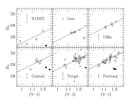
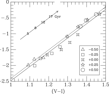
Figure 5: Top panel: fluctuation apparent magnitudes $\overline{m_{I}}$ versus $(V-I)$ color for several nearby groups and clusters. The solid lines drawn through the data points all have slope 4.5. Bottom panel: a plot of the theoretical $\overline{M_{I}}$ versus $(V-I)$ relation, from the stellar population synthesis models of Worthey (1994). The different point types indicate different metallicities relative to the Milky Way, as coded in the inset. For each point type, there are several distinct points, corresponding to different stellar population ages, as indicated by the arrow. The solid line is a fit to the theoretical models with slope fixed at 4.5. The dashed line is the empirical relation, equation 10. Adapted from Tonry et al. (1997).

The correlation of fluctuation magnitude with color is quite strong. Accurate colors are therefore required in order to minimize systematic effects. The possibility that the slope or zero point of this correlation may not be universal, but instead depend on some as yet undetermined galaxy properties as suggested by Tammann (1992), merits further attention. However, Tonry et al. (1997) show that the most likely manifestation of such a problem, a trend with metallicity of residuals from the $\overline{M_{I}}$–$(V-I)$ relation, does not exist. It is reassuring, moreover, that theoretical stellar population synthesis models predict a trend of fluctuation magnitude with color that is very similar to the empirical one. This is shown in the lower panel of Figure 5, in which the population synthesis models of Worthey (1994) are plotted in the $\overline{M_{I}}$–$(V-I)$ plane. The points represent models of various metallicities relative to the Milky Way (indicated by point type as coded in the inset of the figure), and of various ages (the trend with age, at a given metallicity, is indicated by the arrow). The solid line, which has slope 4.5 and an intercept determined by fitting to the theoretical models, is seen to be a reasonable fit. The dashed line is the emprical relation, equation 10. The zero point of the theoretical relation differs from that of the empirical one by only 0.07 mag.

5.2 Results from SBF Surveys

The ramifications of existing SBF data for peculiar velocity surveys and the Hubble constant are preliminary, but they are encouraging in terms of what they portend for the knowledge this method will bring in the near future. In the very early days of peculiar velocity work, Tonry & Davis (1980) and Aaronson et al. (1982) estimated values of $\sim\,$250 km s^-1 for the infall of the Local Group into the Virgo cluster. Model fits to the SBF data for Local Supercluster galaxies confirm this value, and show that it is remarkably insensitive to the assumed density profile around Virgo (Tonry 1995). Another early scientific result of SBF studies has been validation of the large peculiar motions of elliptical galaxies in the Hydra-Centaurus region originally detected using the $D_{n}$-$\sigma$ technique (Dressler 1994). More generally, intercomparison of the SBF and TF/$D_{n}$-$\sigma$ velocity fields in the coming years will provide an important consistency check. Preliminary tests of this sort have shown good agreement to within the quoted errors (Tonry 1995; Tonry et al. 1997).

The zero point of the SBF method (i.e., the value of $\overline{M_{I}}$ for a given $(V-I)$ color) was poorly known until recently, but has now been determined from a comparison of SBF and Cepheid distances. Taking the distances in Mpc to the Local Group, the M81, CenA, NGC 1023, NGC 3379, NGC 7331 groups, and the Virgo cluster from published Cepheid data, Tonry et al. (1997) obtained the zero point given in equation 10. By working with groups, Tonry et al. were able to include 10 galaxies with Cepheid distances and a total of 44 SBF galaxies in the calibration. However, this comparison suffers from the nagging possibility that the SBF objects, which are preferentially ellipticals and S0s, may not lie at precisely the same distances as the Cepheid galaxies, which are late-type spirals, in the same group. Indeed, there are currently only five galaxies with both Cepheid and SBF distances. One of these, NGC 5253, gives a discordant result. If the remaining four are used, Tonry et al. (1997) find an SBF zero point $-1.82\pm 0.06,$ in reasonable agreement with the preferred value of $-1.74\pm 0.05$ found from the group comparison.

Thus calibrated, the SBF technique can be used as a temporary bridge between Cepheid distances, still too few in number to be reliable calibrators, and the secondary DIs that probe the far-field of the Hubble flow. Tonry et al. (1997) used SBF distances for groups and individual galaxies to provide absolute calibrations for TF, $D_{n}$-$\sigma$, and Type Ia supernovae (§6). In so doing, they obtained distances in Mpc for relatively distant galaxies, and thus estimates of the Hubble constant. The mean value was found to be $H_{0}=81\pm 6\ {\rm km}\,{\rm s}^{-1}\,{\rm Mpc}^{-1}$ from SBF-calibrated secondary DIs. Such a large value of $H_{0},$ if it holds up, may prove problematic for Big Bang cosmology, as discussed in §2. However, it should be kept in mind that the absolute calibration of SBF is tied to the Cepheid distance scale, and that the latter might change in coming years as the HST Key Project (§2) continues.

6 Supernovae

The use of supernovae as distance indicators has grown dramatically in the last few years. Supernovae have been applied to the Hubble Constant problem, to measurement of the cosmological parameters $\Omega_{0}$ and $\Lambda,$ and even, in a preliminary way, to constraining bulk peculiar motions. There is every reason to believe that in the next decade supernovae will become still more important as distance indicators. It is certain that many more will be discovered, especially at high redshift.

Supernovae come in two main varieties. Type Ia supernovae (SNe Ia) are thought to result from the nuclear detonation of a white dwarf star that has been overloaded by mass transferred from an evolved (Population II) companion. (Recall that a white dwarf cannot have a masss above the Chandrasekhar limit, $1.4M_{\odot}.$ When mass transfer causes the white dwarf to surpass this limit, it explodes.) Type II supernovae result from the imploding cores of high-mass, young (Population I) stars that have exhausted their nuclear fuel. Of the two, it is the Type Ias that have received the most attention lately. Type IIs have shown somewhat less promise as distance indicators. They are considerably fainter ($\sim\,$2 mag), and thus are detected less often in magnitude limited surveys (although their intrinsic frequency of occurrence is in fact greater than that of Type 1as). The discussion to follow will be restricted to Type Ias.

Because SNe Ias result (in all likelihood) from detonating white dwarfs, and because the latter tend to have very similar masses, SNe Ias tend to have very similar luminosities. That is, they are very nearly standard candles, so comparison of their apparent and abolute magnitudes yields a distance. Recent work suggests that Type Ia SNe are not quite standard candles, in that their peak luminosities correlate with the shape of their light curves (Phillips 1993; Hamuy et al. 1995; Riess, Press, & Kirshner 1995a,b; Perlmutter et al. 1997). Basically, broad light curves correspond to brighter, and narrow light curves to fainter, supernovae. When this effect is accounted for, the scatter in SNe Ia predicted peak magnitudes might be as small as 0.1 mag, as found by Riess, Press, & Kirshner (1995b). Hamuy et al. (1995) and Perlmutter et al. (1997) find that the scatter drops from $\lower 2.15277pt\hbox{$\,\buildrel<\over{\sim}\,$}0.3$ mag mag when SNe Ia are treated as standard candles to 0.17 mag when the light curve shape is taken into account. The precise scatter of SNe Ias remains a subject for further study.

The wealth of new SNe data that has become available in recent years is due to the advent of large-scale, systematic search techniques. To understand this, it may be worth stating the obvious. It is not possible to pick an arbitrary galaxy and get a supernova distance for it because most galaxies, at a given time, do not have a supernova in them. Thus, it is necessary to search many galaxies at random and somehow identify the small fraction ($\sim 10^{-4}$) in which a supernova is going off at any given time. Methods for doing this have been pioneered by Perlmutter and collaborators (Goobar & Perlmutter 1995; Perlmutter et al. 1995, 1996, 1997). Deep images are taken of the same region of the sky 2–3 weeks apart. Stellar objects which appear in the second image but not in the first are candidate supernovae to be confirmed by spectroscopy. By means of such an approach, of order 30 high-redshift ($z=0.35$–0.65) are now known. Related approaches for finding moderate- (Adams et al. 1995; Hamuy et al. 1995) and high- (Schmidt et al. 1995) redshift supernovae have been developed by other groups as well.

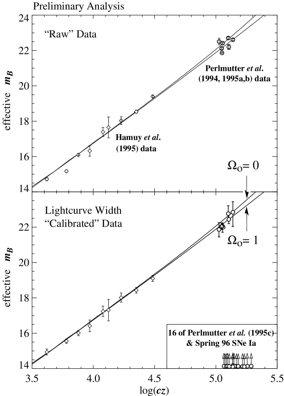
Figure 6: Hubble diagrams using SNe Ia. The upper panel shows the observed peak apparent magnitudes; in the lower panel the magnitudes are corrected for the light curve width effect (see main text for details). The inset in the lower panel shows the redshifts of 16 additional SNe Ias recently discovered but not yet analyzed by the Perlmutter group.

Search techniques such as those of the Perlmutter group survey many faint galaxies in limited regions of the sky, and are not very good at finding low-redshift ($z\lower 2.15277pt\hbox{$\,\buildrel<\over{\sim}\,$}0.03$) supernovae. Thus, they are not particularly relevant to peculiar velocity studies (but see below). However, precisely because they detect intermediate to high redshift supernovae, such techniques will be useful for measuring $H_{0}$ (with supernovae found at $z\lower 2.15277pt\hbox{$\,\buildrel<\over{\sim}\,$}0.2,$ where cosmological effects are relatively unimportant), and are among the best existing methods for determining the cosmological parameters $\Omega_{0}$ and $\Lambda$ (with supernovae at $z\lower 2.15277pt\hbox{$\,\buildrel>\over{\sim}\,$}0.3,$ which probe spatial curvature.) To see how this works, one can plot Hubble diagrams for recently discovered supernovae both at moderate and high redshift. This is done in Figure 6, which has been adapted from the 1996 San Antonio AAS meeting contribution by the Perlmutter group. The low redshift data ($\log(cz)<4.5$) are from Hamuy et al. (1995), and the high redshift data are from Perlmutter et al. (1996).

Figure 6 contains several important features. First, the observed peak apparent magnitudes are plotted versus log redshift in the top panel. To the degree SNe Ias are standard candles, one expects these apparent magnitudes to go as ${\rm const.}+5\log(cz),$ the straight line plotted through the points at low redshift. Correcting the SNe Ia magnitudes for the light curve widths (i.e., going from the top to the bottom panel) significantly improves the agreement with this low-redshift prediction. This is the main reason that the light curve width correction is thought to greatly reduce the SNe Ia scatter. Whether or not the correction is made, however, the data provide unequivocal proof of the linearity of the Hubble law at low ($z\simeq 0.1$) redshift. Second, one expects that that at higher redshifts the $m_{B}$-$\log(cz)$ relation will depart from linearity because of spacetime curvature. The departure from linearity is, to first order in $z,$ a function only of the deceleration parameter $q_{0}$—or equivalently, if the universe has vanishing cosmological constant $\Lambda$ (see below), by the density parameter $\Omega_{0},$ which in that case is exactly twice $q_{0}.$ Figure 6 assumes $\Lambda\equiv 0$ and thus labels the curves by $\Omega_{0}.$ There is a hint in the behavior of the light-curve-shape corrected magnitudes that this departure from linearity has been detected, and in particular that $\Omega_{0}\simeq 1$ is a better fit to the data than $\Omega_{0}\simeq 0$ (Perlmutter et al. 1996).

Neither $q_{0}$ nor $\Omega_{0}$ alone fully characterizes the departure from a linear Hubble diagram. More generally, the behavior of the Hubble diagram at high redshift depends on the cosmological parameters $\Omega_{0}$ and $\Omega_{\Lambda}\equiv\Lambda/3H_{0}^{2}.$ Perlmutter et al. (1997) suggest that the SNe Ia data should be interpreted for now in the context of two cosmological paradigms: a $\Lambda=0$ universe, and a spatially flat ($\Omega_{0}+\Omega_{\Lambda}=1$) universe. Perlmutter et al. (1997) carried out a statistical analysis of the 7 high-redshift ($0.354\leq z\leq 0.458$) supernovae discovered in their survey, and the 9 lower redshift SNe Ias found by the Hamuy group, that are shown in Figure 6. They find that $\Omega_{0}=0.96^{+.56}_{-.50}$ if a $\Lambda=0$ universe is assumed. If the universe is flat, $\Omega_{0}=0.98^{+.28}_{-.24},$ with corresonding limits on $\Omega_{\Lambda}=1-\Omega_{0}.$ The constraints are stronger in the flat universe case because of the strong effect of a cosmological constant on the apparent magnitudes of high-redshift standard candles. These results are, potentially, highly significant for cosmology. Low-density, spatially flat models have become popular lately because they make the universe older (for a given $H_{0}$ and $\Omega_{0}$), provide a better fit to large-scale structure data than $\Omega_{0}=1$ models, and yet remain consistent with the attractive idea that the early universe underwent inflation. Currently favored versions of such models have $\Omega_{\Lambda}\simeq 0.6$–$0.7$ (Ostriker & Steinhardt 1995). The SNe Ia results of Perlmutter et al. (1997), which strongly disfavor such a large $\Omega_{\Lambda},$ will be difficult to reconcile with low-density flat models.

The analysis just described did not require absolute calibration of SNe Ias. Indeed, Perlmutter et al. 1997 use a formalism similar to that used in peculiar velocity studies, in which distances are measured in km s^-1, and absolute magnitudes are, correspondingly, defined only up to an arbitrary constant. The SNe Ia data can be used to determine $H_{0},$ however, only to the degree that the true absolute magnitudes (preferably corrected for light curve width) of such objects are known. This requires either theoretical calibration or empirical calibration in galaxies with Cepheid distances. Both of these approaches pose difficulties. A range of models of exploding white dwarfs predict peak absolute magnitudes for SNe Ias of $M_{V}\simeq-19.5$ with small scatter, but significantly lower luminosities can result if some of the key inputs to the models (especially the mass of the ⁵⁶Ni ejectae) are varied (Höflich, Khokhlov, & Wheeler 1995). This suggests that the absolute magnitudes of SNe Ias cannot yet be predicted theoretically, and that an empirical calibration using Cepheid distances will do better. However, because local galaxies with Cepheid distances are scarce, and SNe Ias are rare, there are still few reliable local calibrators for SNe Ias. It has been necessary to analyze historical as well as modern SNe Ia data (Saha et al. 1995; Sandage et al. 1996) in Cepheid galaxies in order to increase the number of calibrators. This approach encounters the problem of relating modern CCD photometry with photometric methods from decades past. Pending the detection and analysis of SNe Ias in a larger number of local galaxies with Cepheid distances, one should view estimates of $H_{0}$ inferred from supernovae as preliminary.

Being rare events, SNe Ias are unlikely to provide a detailed map of the local peculiar velocity field. However, because of their small scatter (see above), a few well-observed SNe Ias distributed on the sky may lead to useful constraints on amplitude and scale of large-scale bulk flows. A first attempt at this was carried out by Riess, Press, & Kirshner (1995b), who used 13 SNe Ias with peak magnitudes corrected by light curve widths to place limits on the bulk flow within $\sim\,$7000 km s^-1. They found the data to be consistent with at most a small ($\lower 2.15277pt\hbox{$\,\buildrel<\over{\sim}\,$}400\ {\rm km}\,{\rm s}^{-1}$) bulk streaming, and to be inconsistent with the large bulk flow found by Lauer & Postman (1994) using an independent method (cf. §7 below). However, one must be cautious in interpreting such results because small-scale power in the velocity field can obscure large-scale motions (Watkins & Feldman 1995). Constraints on bulk flows using SNe Ias are likely to improve in the coming years.

7 Brightest Cluster Galaxies

Another “classical” distance indicator method that has been reborn in modern guise is photometry of brightest cluster galaxies (BCGs). As originally treated by Sandage and coworkers (Sandage 1972; Sandage & Hardy 1973), BCGs were considered to be good standard candles. As such, they were used to demonstrate the linearity of the Hubble diagram to relatively large distances and estimate $H_{0}.$ Any such estimate was and remains highly suspect, however, because of the difficulty of obtaining a good absolute calibration of the method. The scatter of BCGs as standard candles is around 0.30–0.35 mag, which compares favorably with methods such as TF or $D_{n}$-$\sigma$.

A dubious assumption in the early work was that BCGs are true standard candles. Gunn & Oke (1975) first suggested that the luminosities of BCGs might correlate with their surface brightness profiles. Following this suggestion, Hoessel (1980) defined a metric radius $r_{m}=10h^{-1}$ kpc, and showed that the metric luminosity $L(r_{m})\equiv L_{m}$ varied roughly linearly with a shape parameter $\alpha$ defined by

$$\alpha\equiv\left.\frac{d\log L}{d\log r}\right|_{r_{m}}\,.$$ (11)

More recently, Lauer & Postman (1992) have shown that the correlation between $L_{m}$ and $\alpha$ is better modeled by a quadratic relation. The Lauer & Postman (1992) data, along with their quadratic fit, are shown in the upper panel of Figure 7. Thus modeled, the typical distance error incurred by the BCG $L_{m}$-$\alpha$ relation is $\sim\,$16%.

A slight hitch in applying the BCG $L_{m}$-$\alpha$ relation is the requirement of defining a metric radius $r_{m}$ for evaluating both $L_{m}$ and $\alpha.$ This means that the assumed peculiar velocity of a BCG must be factored in to convert redshift to distance, and thus angular to linear diameter. In practice this is not a very serious issue. At the typically large distances ($\lower 2.15277pt\hbox{$\,\buildrel>\over{\sim}\,$}7000\ {\rm km}\,{\rm s}^{-1}$) at which the relation is applied, peculiar velocity corrections have a small effect on $L_{m}$ and $\alpha.$ Iterative techniques in which a peculiar velocity solution is obtained and then used to modify the $r_{m}$s, converge quickly (Lauer & Postman 1994).

Figure 7: Top panel: the BCG $L_{m}-\alpha$ relation exhibited by the sample of Lauer & Postman (1992). Absolute magnitude within the metric radius $r_{m}$ is plotted against the logarithmic surface brightness slope at $r_{m}.$ The solid curve shows the quadratic fit to the data. Bottom panel: the Hubble diagram for the Lauer & Postman (1992) BCG sample. Apparent magnitude within $r_{m}$ is plotted against log redshift. The straight line plotted through the points has slope 5, the relation expected for a linear Hubble flow. The data used to make this figure were kindly provided by Marc Postman.

Modern scientific results based on BCGs are due to the pioneering work of Lauer and Postman (Lauer & Postman 1992; Lauer & Postman 1994, hereafter LP94; Postman & Lauer 1995). One important—and uncontroversial—such result has been confirmation, with unprecedented accuracy, of the linearity of the Hubble diagram to redshifts $z\simeq 0.05$ over the entire sky. (The Hubble diagrams using SNe Ias (§6), by contrast, are not derived from isotropic samples.) This is shown in the lower panel of Figure 7. However, another result has been considerably more controversial, namely, the detection of a very large-scale bulk peculiar velocity by LP94. The linearity of the BCG Hubble diagram manifests itself with the smallest scatter when the velocities are referred to a local frame that differs significantly from that defined by the CMB dipole. Or, stated another way, the LP94 data indicate that the frame of Abell clusters out to 15,000 km s^-1 redshift is moving with respect to the CMB frame at a velocity of $\sim\,$700 km s^-1 toward $l\simeq 350^{\circ},$ $b\simeq 50^{\circ}.$ A reanalysis of the LP94 data by Colless (1995) produced a very similar result for the bulk motion.

The global Hubble flow linearity demonstrated by Lauer & Postman (1992) suggests that that the BCG $L_{m}$-$\alpha$ relation is an excellent DI out to substantial redshifts. However, the indicated bulk motion is of sufficient amplitude and scale as to appear inconsistent with other indicators of large-scale homogeneity. For example, Strauss et al. (1995) showed that none of the leading models of structure formation that are consistent with other measures of large-scale power can reproduce an LP94-like result in more than a small fraction of realizations. Furthermore, two recent studies, one using the TF relation (Giovanelli et al. 1996) and one using Type Ia SNe (Riess, Press, & Kirshner 1995b), suggest that the bulk motion on smaller scales than that probed by the BCGs is inconsistent with the LP94 bulk flow at high significance levels.

For the above reasons, the current status of BCGs as DIs is controversial. However, one should not prejudge the outcome. Velocity studies have yielded a number of surprises in the last 15 years, and it is not inconceivable that the LP94 bulk flow—or something like it—will be vindicated in the long term. Lauer, Postman, and Strauss are currently extending BCG observations to a complete sample with $z\leq 0.1,$ and the results of their survey are expected to be available by $\sim\,$late 1997. Whether or not it confirms LP94, this extended study is likely to greatly clarify the nature of the BCG $L_{m}$-$\alpha$ relation.

8 Redshift-Distance Catalogs

As redshift measurements accumulated in the 1970s and 1980s, it was widely recognized that there was a need to assemble these data into comprehensive catalogs. Beginning with the publication of the CfA redshift survey in 1983 (Huchra et al. 1983), all major redshift surveys (see the Chapter by Strauss in this volume) led to electronically available databases in fairly short order.

Comparable efforts involving redshift-independent distance measurements have been slower in coming. This is largely due to the issue of uniformity. Whereas redshift measurements by different observers rarely exhibit major differences, redshift-independent distances obtained by different observers can, and generally do, differ systematically for any number of reasons. In some cases the origin of such differences is different calibrations of the DI. In others, the calibrations are the same but the input data differ in a subtle way. Finally, the way statistical bias effects are treated (§9) often differs among those involved in galaxy distance measurements. For all these reasons, it is not possible simply to go to the published literature, find all papers in which galaxy distances are reported, and lump them together in a single database. Instead, individual data sets must be assembled, their input data and selection criteria characterized, their DI relations recalibrated if necessary, and the final distances brought to a uniform system. Only then can the resultant catalog be relied upon—and even then, caution is required.

The first steps toward assembling homogeneous redshift-distance catalogs were taken in the late 1980s by David Burstein. His goal was to combine the then newly-acquired $D_{n}$-$\sigma$ data from the 7-Samurai group (§4) with the extant data on spiral galaxy distances, especially the infrared TF data obtained by the Aaronson group (§3). Burstein’s efforts produced two electronic catalogs, the Mark I (1987) and Mark II (1989) Catalogs of Galaxy Peculiar Velocities. Burstein’s chief concern was matching the TF and $D_{n}$-$\sigma$ distance scales. As there are, by definition, no galaxies that have both kinds of distances, this matching could be carried out through a variety of overlapping approaches. The approach decided upon by Burstein, in consultation with the other 7 Samurai, was to require the Coma cluster spirals and ellipticals to have the same mean distances. Although this procedure was imperfect, the Mark II catalog was considered reliable enough to be used in the first major effort to constrain the density parameter $\Omega_{0}$ by comparing velocities and densities (Dekel et al. 1993).

With the publication of a number of large, new TF data sets in the early 1990s, the need for a greatly expanded redshift-distance catalog became apparent. An important development was the superseding of the majority of the older infrared TF data, obtained by the Aaronson group, by CCD-based ($R$-and $I$-band) TF data. Han, Mould and coworkers (Han 1991, 1992; Han & Mould 1992; Mould et al. 1991, 1993) obtained a full-sky cluster TF sample, based on $I$ -band magnitudes and 21 cm velocity widths, comprising over 400 galaxies. Willick (1990, 1991) and Courteau (1992; Courteau et al. 1993) gathered $R$-band TF data in the Northern sky for over 800 galaxies in total. The largest single contribution was that of Mathewson, Ford, & Buchorn (1992) who published an $I$-band TF sample of 1355 galaxies in the Southern sky. Despite the influx of the new CCD data, one portion of the infrared TF database of the Aaronson group was not rendered obsolete: the sample of over 300 local ($cz\lower 2.15277pt\hbox{$\,\buildrel<\over{\sim}\,$}3000\ {\rm km}\,{\rm s}^{-1}$) galaxies first observed in the late 1970s and early 1980s (Aaronson et al. 1982). This local sample was, however, subjected to a careful reanalysis by Tormen & Burstein (1995), who rederived the $H$-band magnitudes using a more homogeneous set of galaxy diameters and inclinations than was available to the original researchers a decade earlier.

In 1993, a group of astronomers (myself, Burstein, Avishai Dekel, Sandra Faber, and Stéphane Courteau) began the process of integrating these TF data and the existing $D_{n}$-$\sigma$ data into a new redshift-distance catalog. Our methodology is described in detail in Willick et al. (1995, 1996), and portions of the catalog are presented in Willick et al. (1997). The full catalog, known as the Mark III Catalog of Galaxy Peculiar Velocities, is quite large (nearly 3000 spirals and over 500 ellipticals, although this includes several hundred overlaps between data sets) and is available only electronically, as described in Willick et al. (1997).

Building upon the foundation laid by Burstein in the Mark I and II catalogs, the Mark III catalog was assembled with special emphasis placed on achieving uniform distances among the separate samples it comprises. Four specific steps were taken toward this goal. First, the raw data in all of the TF samples underwent a uniform set of corrections for inclination and extinction (cf. §3.2). Second, the TF relations for each sample were recalibrated using a self-consistent procedure that included correction for selection bias (§9). Third, final TF zero points were assigned by requiring that the TF distances of objects common to two or more samples agree in the mean. This step ensures that the different samples are on similar relative distance scales. The global TF zero point was determined by the fully-sky Han-Mould cluster TF sample. (As explained in §3, this zero point was such that the distances are given in units of km s^-1, not Mpc.) Fourth, the spiral and elliptical distance scales were matched by applying the POTENT algorithm (see the chapter by Dekel in this volume) to each separately, and requiring that they produce statistically consistent velocity fields.

In parallel with the efforts of the Mark III group, similar enterprises have been undertaken by two other groups. Brent Tully has also assembled and recalibrated much of the extant TF data. Riccardo Giovanelli, Martha Haynes, Wolfram Freudling, Luiz da Costa, and coworkers have acquired new $I$ band TF data for $\sim\,$2000 galaxies, and have combined it with the sample of Mathewson et al. 1992). Initial scientific results from each of these efforts have been published (Shaya, Tully, & Peebles 1995; Giovanelli et al. 1996; da Costa et al. 1996), and the catalogs themselves will soon become publically available.

New distances for elliptical galaxies, now mostly from the FP rather than $D_{n}$-$\sigma$ (§ 4), continue to be obtained as well. Jorgensen, Franx, & Kjaergaard (1995a,b) have published distances for E and S0 galaxies in 10 clusters out to 10,000 km s^-1. The EFAR group (Burstein, Colless, Davies, Wegner, and colleagues) are now finishing an FP survey of over 80 groups and clusters at distances between 7000 and 16,000 km s^-1 (Colless et al. 1993; Wegner et al. 1993,1996; Davies et al. 1993).

Implicit in all this ongoing work is that the Mark III catalog, like its predecessors, is just one step along a path still being traveled. Just as the Mark III data consists in part of recalibrated data alreay present in the Mark II, so will future catalogs incorporate, partially recalibrate, and expand upon the Mark III. Of particular note are the distances coming from the SBF survey of Tonry and coworkers (Tonry et al. 1997; cf. §5). The SBF distances are much more accurate than either TF or $D_{n}$-$\sigma$ and can provide important checks on them. Tonry et al. (1997) have taken initial steps toward such an intercomparison, and the preliminary results, which suggest mutally consistent results among SBF, $D_{n}$-$\sigma$, and TF, are encouraging. Little comparison of SNe and BCG distances with other DIs has yet been carried out, but will be in the coming years. It is reasonable to hope that, by the turn of the century at the latest, the available redshift-distance catalogs will be superior, in terms of sky coverage, accuracy, and homogeneity, to the best we have today.

9 Malmquist and Other Biases

Distance scale and peculiar velocity work have long been plagued by statistical biases. These biases are sufficiently confusing and multifaceted that their effects are often misunderstood or misrepresented. It is worth taking a moment to go over a few of the main issues.

The root problem is that our distance indicators contain scatter: a galaxy with distance $d$ inferred from the DI really lies within some range of distances, approximately (but not exactly) centered on $d.$ This range is characterized by a non-gaussian distribution of characteristic width $d\Delta,$ where $\Delta$ is the fractional distance error characteristic of the DI. (If $\sigma$ is the DI scatter in magnitudes, $\Delta\simeq 0.46\sigma$). Thus, the farther away the object is the bigger the distance error. For most DIs, a good approximation is that the distribution of distance errors is log-normal: if the true distance is $r,$ then the distance estimate $d$ has a probability distribution given by

$$P(d|r)=\frac{1}{\sqrt{2\pi}(d\Delta)}\exp\left[-\frac{\left[\ln(d/r)\right]^{2}}{2\Delta^{2}}\right]\,.$$ (12)

Two distinct kinds of statistical bias effects can arise when DIs with the above properties are used. Which of the two occurs depends on which of two basic analytic approaches one adopts for treating the DI data. In the first approach, known as Method I, one assumes that the DI-inferred distance $d$ is the best a priori estimate of true distance. Any subsequent averaging or modeling of the data points assumes galaxies with similar values of $d$ to be neighbors in real space as well. The second approach, known as Method II, takes proximity in redshift space as tantamount to real-space proximity; the DI-inferred distances are then treated only in a statistical sense, averaged over objects with similar redshift-space positions. The Method I/Method II terminology originated with Faber & Burstein (1988); a detailed discussion is provided by Strauss & Willick (1995, §6.4).

Let us consider this distinction in relation to peculiar velocity or Hubble constant studies. In a Method I approach, one would take objects whose DI-inferred distances are within a narrow range of some value $d,$ and average their redshifts. Subtracting $d$ from the resulting mean redshift yields a peculiar velocity estimate; dividing the mean redshift by $d$ gives an estimate of $H_{0}.$ However, these estimates will be biased, because the distance estimate $d$ itself is biased: It is not the mean true distance of the objects in question. To see this, we reason as follows: if $P(d|r)$ is given by equation (12) above, then the distribution of true distances of our objects is given, according to Bayes’ Theorem, by

$$P(r|d)=\frac{P(d|r)P(r)}{\int_{0}^{\infty}P(d|r)P(r)\,dr}=\frac{r^{2}n(r)\exp\!\left(-\frac{\left[\ln r/d\right]^{2}}{2\Delta^{2}}\right)}{\int_{0}^{\infty}r^{2}n(r)\exp\!\left(-\frac{\left[\ln r/d\right]^{2}}{2\Delta^{2}}\right)\,dr}\,,$$ (13)

where we have taken $P(r)\propto r^{2}n(r),$ where $n(r)$ is the underlying galaxy number density along the line of sight. To obtain the expectation value of the true distance $r$ for a given $d,$ we multiply equation (13) by $r$ and integrate over all $r.$ In general, this integral requires knowledge of the density field $n(r)$ and will have to be done numerically. However, in the simplest case that the density field is constant, the integral can be done analytically. The result is that the expected true distance is $de^{7\Delta^{2}/2}$ (Lynden-Bell et al. 1988; Willick 1991). This effect is called homogeneous Malmquist bias. It tells us that, typically, objects lie further away than their DI-inferred distances. The physical cause is more objects “scatter in” from larger true distances (where there is more volume) than “scatter out” from smaller ones. In general, however, variations in the number density cannot be neglected. When this is the case, there is inhomogeneous Malmquist bias (IHM). IHM can be computed numerically if one has a model of the density field. Further discussion of this issue may be found in Willick et al. (1997).

The biases which arise in a Method II analysis are quite different. They may be rigorously understood in terms of the probability distribution of the DI-inferred distance $d$ given the redshift $cz,$ $P(d|cz)$ (contrast with equation 13, which underlies Method I). In general, this distribution is quite complicated (cf. Strauss & Willick 1995, §8.1.2), and its details are beyond the scope of this Chapter. However, under the assumption of a “cold” velocity field—an assumption that appears adequate in ordinary environments—redshifts complemented by a flow model give a good approximation of true distance. Thus, it really is the probability distribution $P(d|r)$ (equation (12), or one similar to it, that counts for a Method II analysis. However, that equation as written does not represent the full story. If severe selection effects such as a magnitude or diameter limit are present, then the log-normal distribution does not apply exactly. Some galaxies are too faint or small to be in the sample; in effect, the large-distance tail of $P(d|r)$ is cut off. It follows that the typical inferred distances are smaller than those expected at a given true distance $r.$ As a result, the peculiar velocity model that allows true distance to be estimated as a function of redshift is tricked into returning shorter distances. This bias goes in the same sense as Malmquist bias, but is fundamentally different. It results not from volume/density effects, but from sample selection effects, and is called selection bias.

Selection bias can be avoided, or at least minimized, by working in the so-called “inverse direction.” What that means is most easily illustrated using the TF relation. When viewed in its “forward” sense, the TF relation is conceived as a prediction of absolute magnitude given a value of the velocity width parameter, $M(\eta).$ However, it is equally valid to view the relation as a prediction of $\eta$ given a value of $M,$ i.e., as a function $\eta^{0}(M)$ (the superscript ensures that there is no confusion between the observed width parameter $\eta$ and the TF-prediction). When one uses the forward relation, one imagines fitting a line $m_{i}=M(\eta_{i})+\mu$ by regressing the apparent magnitudes $m_{i}$ on the velocity widths $\eta_{i}$; the distance modulus $\mu$ is the free parameter solved for. Selection bias then occurs because apparent magnitudes fainter than the magnitude limit are “missing” from the sample, so the fitted line is not the same as the true line. However, if one instead fits a line $\eta^{0}(m_{i}-\mu)$ by regressing the widths on the magnitudes, the same effect does not occur, provided the sample selection procedure does not exclude large or small velocity widths. In general, this last caveat is more or less valid. Consequently, working in the inverse direction does in fact avoid or at least minimize selection bias.

This fact, first clearly stated by Schechter (1980) and then reiterated in various forms by Aaronson et al. (1982), Tully (1988), Willick (1994), Dekel (1994), and Davis, Nusser, & Willick (1996), among others, remains an obscure one, not universally appreciated. It is often heard, for example, that the TF relation applied to relatively distant galaxies will necessarily result in a Hubble constant that is biased high, because the distances are biased low due to selection bias. The clear conclusion of the previous paragraph, however, is that provided the analysis is done using redshift-space information to assign a priori distances—that is, provided that a Method II approach is taken—working in the inverse direction can render selection bias unimportant. It is also the case that a careful analytical methods (Willick 1994) can permit a correction for selection bias even when working in the forward direction. It should be borne in mind, however, that both of these approaches (using the inverse relation or correction for forward selection bias) necessitate a careful characterization of sample selection criteria.

“Method Matrix” of Distance Indicator Biases DI type/Method Type Method I Method II DI-inferred distance best Redshift-space data best indicator of true distance indicator of true distance Forward Malmquist bias Strong selection bias dist-dep (e.g. mag) predicted (selection-independent (depends on observation al by dist-indep (e.g. $\eta$) quantity selection criteria) Inverse Malmquist bias Weak or no selection bias dist-indep predicted (selection-dependent) (bias present if selection by dist-dep quantity related to dist-indep quantity)

Another wrinkle in this complicated subject is that the relatively bias-free character of inverse distance indicators does not carry over to a Method I analysis. It is beyond the scope of this Chapter to discuss this issue in full detail; the interested reader is referred to Strauss & Willick (1995, § 6.5). The main point is that a Method I inverse DI analysis is subject to Malmquist bias in much the same way as a Method I forward analysis; indeed, the inverse Malmquist bias is in some ways considerably more complex, as it depends (unlike forward Malmquist bias) on sample selection criteria. So while it is correct to emphasize the bias-free (or nearly so) nature of working in the inverse direction, it is essential to remember that this property holds only for Method II analyses.

Much of the confusion surrounding the relative bias properties of forward versus inverse DIs stems from neglecting the distinction between Method I and Method II analyses. Recognizing this, Strauss & Willick (1995) summarized the issue with what they called the “Method Matrix” (a more memorable term might be the “magic square”) of peculiar velocity analysis. Their table is reproduced above, in a slightly simpler form (the original alluded to several complications that are unecessary here). Reference to this simple diagram might allay some of the controversies surrounding Malmquist and related biases.

10 Summary

The measurement of galaxy distances is crucial for some of the basic problems in astronomy and cosmology. In this Chapter I have emphasized the role such measurements play in two of the most important: Hubble constant determination and peculiar velocity analysis. An important distinction between these two efforts, which I have reiterated throughout, is that for peculiar velocities one only needs distances in km s^-1, which are independent of an absolute distance scale, whereas for determination of $H_{0}$ distances in Mpc are required. In practice, this means that peculiar velocity studies may be carried out using distance indicators such as TF or $D_{n}$-$\sigma$ calibrated only relative to the distant Hubble flow. To obtain $H_{0}$ the same DIs must be calibrated relative to local galaxies with Cepheid distances. Because the program of Cepheid measurements in local calibrators using HST (Kennicutt et al. 1995) is ongoing, reliable far-field measurements of $H_{0}$ are still several years away.

I have organized the discussion around the principal distance indicators currently in use. These are:

1. Cepheid variables. The Period-Luminosity relation for these pulsating stars may be calibrated in the Milky Way and in the Magellanic Clouds. However, they are detectable with HST out to $\sim\,$20 Mpc. As such, they will yield accurate absolute distances for $\sim\,$20 local galaxies over the next several years. These local galaxies will in turn provide absolute calibrations for the secondary distances indicators such as TF or SNe Ia that will be used to measure $H_{0}$ in the “far field” ($\lower 2.15277pt\hbox{$\,\buildrel>\over{\sim}\,$}7000\ {\rm km}\,{\rm s}^{-1}$), where peculiar velocities and depth effects are relatively unimportant.

2. The TF relation. This method has been the workhorse of peculiar velocity studies, for it applies to the ordinary spiral galaxies that best trace the peculiar velocity field. When calibrated using HST Cepheid distances, it promises also to yield a value of $H_{0}$ accurate to $\sim\,$10%. The TF relation has recently been shown to apply to spiral galaxies at high redshift (Vogt et al. 1996), although evolutionary effects appear to be significant at $z\simeq 0.5.$

3. The $D_{n}$-$\sigma$ relation. This is a variant of the Fundamental Plane relations for elliptical galaxies. It is comparable to TF in accuracy, and gives similar global results for the large-scale peculiar velocity field (Kolatt & Dekel 1994). Its best chance for absolute calibration comes from a comparison with SBF distances. Like TF, $D_{n}$-$\sigma$ has recently been applied to relatively high redshift galaxies (Bender et al. 1996), again with evidence of evolutionary changes.

4. Surface Brightness Fluctuations (SBF). This method may be the most accurate DI known for galaxies beyond the range of HST Cepheid measurements, with distance errors as small as 5% under the best conditions and median errors of $\sim\,$8%. Its application is most straightforward for early-type systems, although with care it may be applied to spirals as well. It holds the promise of giving a high-resolution picture of the peculiar velocity field. It will also provide a crucial check of the reliability of TF and $D_{n}$-$\sigma$. Its direct application to the $H_{0}$ problem remains uncertain because of the great technical challenge involved in extending it to distances $\lower 2.15277pt\hbox{$\,\buildrel>\over{\sim}\,$}5000\ {\rm km}\,{\rm s}^{-1}.$

5. Type Ia Supernovae. SNe are in principle excellent DIs, but suffer from the obvious problem that one cannot, in general, be found in a given galaxy at a given time. In recent years, improved search techniques have vastly increased the number of well-observed SNe Ias, both at relatively low (Hamuy et al. 1995) and high (Perlmutter et al. 1996) redshifts. The results of these studies have included beautiful Hubble diagrams that demonstrate the linearity of the Hubble expansion to $z\simeq 0.1,$ with tantalizing hints of curvature that hold the promise of constraining the cosmological parameters $\Omega_{0}$ and $\Lambda.$ Sandage and coworkers (Sandage et al. 1996; Saha et al. 1995) have calibrated SNe Ias in galaxies with Cepheid distances to obtain Hubble constant estimates of $H_{0}\simeq 57\ {\rm km}\,{\rm s}^{-1}\,{\rm Mpc}^{-1}.$ However, considerable uncertainty attaches to these results at present. The quest for a reliable absolute calibration of SNe Ias continues.

6. The BCG $L_{m}$-$\alpha$ relation. The pioneering work of Lauer and Postman (Lauer & Postman 1992, 1994; Postman & Lauer 1995) has demonstrated the potential of BCGs in distance scale and peculiar velocity work. The detection of very large-scale bulk streaming using BCGs has caused some to question the global validity of the $L_{m}$-$\alpha$ relation (e.g., Riess, Press, & Kirshner 1995b), but the verdict is not in yet. Ongoing work by Lauer and Postman, in collaboration with Strauss, will greatly clarify the situation.

I conclude by reiterating a point made at the outset of this Chapter. The DIs discussed here are empirical relations whose physical origins are only partially understood at best. There is a class of distance indicators that are based on fairly rigorous physics, and whose absolute calibration may be obtained from first principles. Gravitational lensing of time-variable quasars and the Sunyaev-Zeldovich effect in clusters are perhaps the most noteworthy of these. It is conceivable that these methods will mature in the coming decade and add greatly to what we have learned from the empirical DIs about the distance scale and the peculiar velocity field. However, this additional information will most likely reinforce, rather than supplant, the knowledge obtained from the DIs discussed here.

Acknowledgments: I would like to thank David Burstein, Tod Lauer, Marc Postman, Saul Perlmutter, and John Tonry for enlightening discussions about the distance indicator relations in which they are leading experts, and for providing me with data or postscript for several of the figures presented here.

References

- (1) Aaronson, M., Huchra, J., & Mould, J. (1979), ApJ, 229, 1
- (2)
- (3) Aaronson, M., Huchra, J., Mould, J., Sullivan, W., Schommer, R., & Bothun, G. (1980), ApJ, 239, 12
- (4)
- (5) Aaronson, M., Huchra, J., Mould, J., Schechter, P.L., & Tully, R.B. (1982), ApJ, 258, 64
- (6)
- (7) Aaronson, M., Bothun, G., Mould, J., Huchra, J., Schommer, R.A., & Cornell, M.E. (1986), ApJ, 302, 536
- (8)
- (9) Adams, M.T., Wheeler, J.C., Ward, M., Wren, W.R., & Schmidt, B.P. (1995), BAAS, 187, 1711
- (10)
- (11) Bender, R., Burstein, D., & Faber, S.M. (1992), ApJ, 399, 462
- (12)
- (13) Bender, R., Burstein, D., & Faber, S.M. (1993), ApJ, 411, 153
- (14)
- (15) Bender, R., Ziegler, B., & Bruzual, G. (1996), ApJ, 463, L51
- (16)
- (17) Baum, W. (1955), PASP, 67, 328
- (18)
- (19) Bernstein, G.M., Guhathakurta, P., Raychaudhury, S., Giovanelli, R., Haynes, M.P., Herter, T., & Vogt, N.P. (1994), AJ, 107, 1962
- (20)
- (21) Bothun, G.D., & Mould, J.R. (1987), ApJ, 313, 629
- (22)
- (23) Bottinelli, L., Gouguenheim, L., Paturel, G., & de Vaucouleurs, G. (1983), A&A, 118, 4
- (24)
- (25) Burstein, D., Willick, J., & Courteau, S. (1995), in Opacity of Spiral Disks, NATO Ser., ed. J.A. Davies & D. Burstein (Dordrecht:Kluwer)
- (26)
- (27) Colless, M., Saglia, R.P., Baggley, G., Burstein, D., McMahan, R.K., Wegner, G., Davies, R.L. & Bertschinger, E. (1993), MNRAS, 262, 475
- (28)
- (29) Colless, M.M. (1995), AJ, 109, 1946
- (30)
- (31) Courteau, S. (1992), Ph.D. Thesis, University of California, Santa Cruz
- (32)
- (33) Courteau, S., Faber, S.M., Dressler, A., & Willick, J.A. (1993), ApJ, 412, L51
- (34)
- (35) Davis, M., Nusser, A., & Willick, J.A. (1996), ApJ, accepted
- (36)
- (37) Dekel, A. (1994), ARA&A, 32, 371
- (38)
- (39) Djorgovski, S., & Davis, M. (1987), ApJ, 313, 59
- (40)
- (41) Dressler, A. (1994), in Cosmic Velocity Fields, eds. F. Bouchet & M. Lachièze-Rey, (Gif-sur-Yvette: Editions Frontières), p. 9
- (42)
- (43) Dressler, A., Lynden-Bell, D., Burstein, D., Davies, R. L., Faber, S. M., Terlevich, Wegner, G. (1987), ApJ, 313, 42
- (44)
- (45) Eastman, R.G., Schmidt, B.P., & Kirsher, R. (1996), ApJ, 466, 911
- (46)
- (47) Eisenstein, D.J., & Loeb, A. (1996), ApJ, 459, 432
- (48)
- (49) Faber, S. M., & Jackson, R. E. (1976), ApJ, 204, 668
- (50)
- (51) Faber, S. M., Dressler, A., Davies, R. L., Burstein, D., Lynden-Bell, D., Terlevich, R. J., & Wegner, G. (1987), in Nearly Normal Galaxies, ed. S. M. Faber (New York: Springer), p. 175
- (52)
- (53) Faber, S.M., & Burstein, D. (1988), in Large Scale Motions in the Universe, ed. V.C. Rubin & G.V. Coyne (Princeton: Princeton University Press), p. 115
- (54)
- (55) Federspiel, M., Sandage, A., & Tammann, G.A. (1994), ApJ, 430, 29
- (56)
- (57) Ferrarese, L., et al. (1996), ApJ, 464, 568
- (58)
- (59) Fisher, A., Branch, D., & Nugent, P. (1993), BAAS, 183, #38.03
- (60)
- (61) Freedman, W.L., & Madore, B.F. (1990), ApJ, 365, 186
- (62)
- (63) Freedman, W.L., Wilson, C.D., & Madore, B.F. (1991), ApJ, 372, 455
- (64)
- (65) Freedman, W.L., et al. (1994), Nature, 371, 757
- (66)
- (67) Freudling, W., da Costa, L.N., Wegner, G., Giovanelli, R., Haynes, M.P., & Salzer, J.J. (1995), AJ, 110, 920
- (68)
- (69) Giovanelli, R., Haynes, M.P., Salzer, J.J., Wegner, G., da Costa, L.N., & Freudling, W. (1995), AJ, 110, 1059
- (70)
- (71) Giovanelli, R., Haynes, M.P., Wegner, G., da Costa, L.N., Freudling, W., & Salzer, J.J. (1996), ApJ, 464, L99
- (72)
- (73) Goobar, A., & Perlmutter, S. (1995), ApJ, 450, 14
- (74)
- (75) Gunn, J.E., & Oke, J.B. (1975), ApJ, 195, 255
- (76)
- (77) Hamuy, M., Phillips, M.M., Maza, J., Suntzeff, N.B., Schommer, R.A., & Aviles, R. (1995), AJ, 109, 1
- (78)
- (79) Han, M.-S. (1992), ApJ, 391, 617
- (80)
- (81) Han, M.-S., & Mould, J.R. (1992), ApJ, 396, 453
- (82)
- (83) Hoessel, J.G. (1980), ApJ, 241, 493
- (84)
- (85) Höflich, P., Khokhlov, A.M., & Wheeler, J.C. (1995), ApJ, 444, 831
- (86)
- (87) Huchra, J., Davis, M., Latham, D., & Tonry, J. (1983), ApJS, 52, 89
- (88)
- (89) Jorgensen, I., Franx, M., & Kjaergaard, P. (1996), MNRAS, 280, 167
- (90)
- (91) Kennicutt, R.C., Freedman, W.L., & Mould, J.R. (1995), AJ, 110, 1476
- (92)
- (93) Kolatt, T., & Dekel, A. (1994), ApJ, 428, 35
- (94)
- (95) Lauer, T.R., & Postman, M. (1992), ApJ, 400, L47
- (96)
- (97) Lauer, T.R., & Postman, M. (1994), ApJ, 425, 418
- (98)
- (99) Lynden-Bell, D., Faber, S. M., Burstein, D., Davies, R. L., Dressler, A., Terlevich, R. J., & Wegner, G. (1988), ApJ, 326, 19
- (100)
- (101) Mathewson, D.S., Ford, V.L, & Buchhorn, M. (1992), ApJS, 81, 413
- (102)
- (103) Montes, M.J., & Wagoner, R.V. (1995), ApJ, 445, 828
- (104)
- (105) Mould, J.R., et al. (1995), ApJ, 449, 413
- (106)
- (107) Ostriker, J.P., & Steinhardt, P.J. (1995), Nature, 377, 600
- (108)
- (109) Pahre, M.A., Djorgovski, S.G., & de Carvalho, R.R. (1995), ApJ, 453, L17
- (110)
- (111) Perlmutter, S., et al. (1995), ApJ, 440, L41
- (112)
- (113) Perlmutter, S., et al. (1996), to appear in Thermonuclear Supernovae, (NATO ASI), eds. R. Canal, P. Ruiz-LaPuente, & J. Isern
- (114)
- (115) Perlmutter, S., et al. (1997), ApJ, in press
- (116)
- (117) Phillips, M.M. (1994), ApJ, 413, L105
- (118)
- (119) Pierce, M.J., & Tully, R.B. (1988), ApJ, 330, 579
- (120)
- (121) Pierce, M.J., & Tully, R.B. (1992), ApJ, 387, 47
- (122)
- (123) Postman, M., & Lauer, T.R. (1995), ApJ, 440, 28
- (124)
- (125) Rephaeli, Y. (1995), ARA&A, 33, 541
- (126)
- (127) Riess, A.G., Press, W.H., & Kirshner, R.P. (1995a), ApJ, 438, L17
- (128)
- (129) Riess, A.G., Press, W.H., & Kirshner, R.P. (1995b), ApJ, 445, L91
- (130)
- (131) Rix, H.-W., Guhathakurta, P., Colless, M., & Ing, K. (1996), MNRAS, submitted
- (132)
- (133) Saglia, R.P., Bertschinger, E., Baggley, G., Burstein, D., Colless, M., Davies, R.L., McMahan, R.K. & Wegner, G. (1993), MNRAS, 264, 971
- (134)
- (135) Saha, A., Sandage, A., Labhardt, L., Schwengeler, H., Tammann, G.A., Panagia, N., & Macchetto, F.D. (1995), ApJ, 438, 8
- (136)
- (137) Sandage, A. (1972), ApJ, 178, 1
- (138)
- (139) Sandage, A., & Hardy, E. (1973), ApJ, 183, 743
- (140)
- (141) Sandage, A. (1994), ApJ, 430, 13
- (142)
- (143) Sandage, A., Saha, A., Tammann, G.A., Labhardt, L., Panagia, N., & Macchetto, F.D. (1996), ApJ, 460, L15
- (144)
- (145) Schechter, P. L. (1980), AJ, 85, 801
- (146)
- (147) Schlegel, D. (1996), Ph.D. Thesis, University of California, Berkeley
- (148)
- (149) Schmidt, B.P., et al. (1995), Aiguiblava NATO ASI Proceedings
- (150)
- (151) Strauss, M.A., & Willick, J.A. 1995, Physics Reports, 261, 271
- (152)
- (153) Strauss, M.A., Cen, R., Ostriker, J.P., Lauer, T.R., & Postman, M. (1995), ApJ, 465, 534
- (154)
- (155) Tammann, G.A., & Sandage, A. (1995), ApJ, 452, 16
- (156)
- (157) Tammann, G.A. (1992), Phys. Scr., T43, 31
- (158)
- (159) Tonry, J., & Davis, M. (1981), ApJ, 246, 680
- (160)
- (161) Tonry, J.L.,& Schneider, D.P. (1988), AJ, 96, 807
- (162)
- (163) Tonry, J.L., Ajhar, E.A., & Luppino, G.A. (1989), ApJ, 346, L57
- (164)
- (165) Tonry, J.L., Ajhar, E.A., & Luppino, G.A. (1990), AJ, 100, 1416
- (166)
- (167) Tonry, J.L., & Schechter, P.L. (1990), AJ, 100, 1794
- (168)
- (169) Tonry, J.L. (1991), ApJ, 373, L1
- (170)
- (171) Tonry, J.L. (1995), Lecture delivered at the Heron Island Workshop on Peculiar Velocities in the Universe (http://qso.lanl.gov/heron)
- (172)
- (173) Tonry, J.L., Blakeslee, J.P., Ajhar, E.A., & Dressler, A. (1997), ApJ, submitted
- (174)
- (175) Tormen, B., & Burstein, D. (1995), ApJS, 96, 123
- (176)
- (177) Tully, R.B., & Fisher, J.R. (1977), A&A, 54, 661
- (178)
- (179) Tully, R.B. (1988), Nature, 334, 209
- (180)
- (181) Vogt, N.P., Forbes, D.A., Phillips, A.C., Gronwall, C., Faber, S.M., Illingworth, G.D., & Koo, D.C. (1996), ApJ, 465, L15
- (182)
- (183) Watkins, R., & Feldman, H.A. (1995), ApJ, 453, L73
- (184)
- (185) Wegner, G., Colless, M., Baggley, G., Davies, R.L., Bertschinger, E., Burstein, D., McMahan, R.K., & Saglia, R.P. (1996), ApJS, accepted
- (186)
- (187) Willick, J.A. (1990), ApJ, 351, L5
- (188)
- (189) Willick, J.A. (1991), Ph.D. Thesis, University of California, Berkeley
- (190)
- (191) Willick, J.A. (1994), ApJS, 92, 1
- (192)
- (193) Willick, J.A., Courteau, S., Faber, S.M., Burstein, D., & Dekel, A. (1995), ApJ, 446, 12
- (194)
- (195) Willick, J.A., Courteau, S., Faber, S.M., Burstein, D., Dekel, A., & Kolatt, T. (1996), ApJ, 457, 460
- (196)
- (197) Willick, J.A., Courteau, S., Faber, S.M., Burstein, D., Dekel, A., & Strauss, M.A. (1997), ApJS, submitted
- (198)
- (199) Worthey, G. (1994), ApJS, 95, 107