A Robust Determination of the Time Delay in 0957+561A,B and a Measurement of the Global Value of Hubble’s Constant

Abstract

Continued photometric monitoring of the gravitational lens system 0957+561A,B in the $g$ and $r$ bands with the Apache Point Observatory (APO) 3.5 m telescope during 1996 shows a sharp $g$ band event in the trailing (B) image light curve at the precise time predicted in an earlier paper. The prediction was based on the observation of the event during 1995 in the leading (A) image and on a differential time delay of 415 days. This success confirms the so called “short delay”, and the absence of any such feature at a delay near 540 days rejects the “long delay” for this system, thus resolving a long standing controversy. A series of statistical analyses of our light curve data yield a best fit delay of $417\pm 3$ days (95% confidence interval) and demonstrate that this result is quite robust against variations in the analysis technique, data subsamples and assumed parametric relationship of the two light curves.

Recent improvements in the modeling of the lens system (consisting of a galaxy plus a galaxy cluster) allow us to derive a value of the global (at $z=0.36$) value of Hubble’s constant $H_{0}$ using Refsdal’s method, a simple and direct (single step) distance determination based on experimentally verified and securely understood physics and geometry. The result is $H_{0}=64\pm 13$ km/s/Mpc (for $\Omega=1$) where this 95% confidence interval is dominantly due to remaining lens model uncertainties. However, it is reassuring that available observations of the lensing mass distribution over constrain the model and thus provide an internal consistency check on its validity. We argue that this determination of the extragalactic distance scale (10% accurate at 1$\sigma$) is now of comparable quality, in terms of both statistical and systematic uncertainties, to those based on more conventional techniques.

Finally, we briefly discuss the prospects for improved $H_{0}$ determinations using gravitational lenses and some other possible implications and uses of the 0957+561A,B light curves.

1 Introduction

More than 30 years ago, Refsdal (1964, 1966) pointed out that the differential light propagation time delay between two or more gravitationally lensed images of a background object establishes an absolute physical distance scale ($c\Delta t$) in the system. Thus, the distance to a high-redshift object is directly measured, yielding a value of Hubble’s constant, $H_{0}$. The theory of this technique has been elaborately developed and its realization has become a major focus of gravitational lens studies [Narayan (1991) gives an especially elegant treatment; see Blandford & Narayan (1992) and Narayan & Bartelmann (1996) for reviews].

It may be useful to briefly review the main strengths of the lensing method in determination of the extragalactic distance scale:

1. It is a geometrical method based on the well understood and experimentally verified physics of General Relativity in the weak-field limit. By contrast, most conventional astronomical techniques for measuring extragalactic distances rely either on empirical relationships or on our understanding of complex astrophysical processes, or both.

2. It provides a direct, single step measurement of $H_{0}$ for each system and thus avoids the propagation of errors along the “distance ladder” which is no more secure than its weakest rung.

3. It measures distances to cosmologically distant objects, thus precluding the possibility of confusing a local with a global expansion rate. Note that both observed CMB fluctuations and COBE normalized numerical simulations of large-scale structure formation suggest the possibility of 10-20% rms expansion rate fluctuations even on scales of order 10,000 km/s for some cosmological models (D. Spergel 1996, private communication; Turner, Cen & Ostriker 1992).

4. Independent measurement of $H_{0}$ in two or more lens systems with different source and lens redshifts allows a powerful internal consistency check on the answer. Although an inaccurate model of the lens mass distribution or other systematic problems could yield an incorrect distance in any particular system, no known or imagined problem will consistently give the same wrong answer when applied to different lenses. Thus, if a small number of time delay measurements all give the same $H_{0}$, this value can be regarded as correct with considerable confidence.

Despite these potent virtues, the practical realization (i.e., at a useful and competitive accuracy) of Refsdal’s method for measuring $H_{0}$ has proven quite challenging and has been long delayed. For the lens system 0957+561A,B (Walsh, Carswell & Weymann 1979), by far the best studied case, there are two basic reasons. First, there has been sufficient ambiguity in detailed models of the mass distribution in the lensing galaxy and associated cluster to allow values of $H_{0}$ different by a factor of two or more to be consistent with the same measured time delay (Young et al. 1981; Narasimha, Subramanian & Chitre 1984; Falco, Gorenstein & Shapiro 1991; Kochanek 1991); fortunately, this problem has been much alleviated by recent theoretical and observational work. See § 4 for details. Second, despite extensive optical (Lloyd 1981; Keel 1982; Florentin-Nielsen 1984; Schild & Cholfin 1986; Vanderriest et al. 1989; Schild & Thomson 1995) and radio (Lehár et al. 1992; Haarsma et al. 1996) monitoring programs extending over a period of more than 15 years, values of the differential time delay discrepant by more than 30% have continued to be debated in the literature. In particular, most studies have given a delay either in the range 400–420 days or one of about 530–540 days. These two rough values, the “short delay” and the “long delay” have been obtained both by applying the same statistical techniques to different data sets and by applying different statistical techniques to the same data [Vanderriest et al. 1989; Lehár et al. 1992; Press, Rybicki & Hewitt 1992a, 1992b (hereafter collectively referred to as PRH); Pelt et al. 1994, 1996 (hereafter collectively PHKRS); Beskin & Oknyanskij 1995]! Moreover, even application of a single technique to a single (radio) data set has produced best estimate delays that move far outside the nominal formal high confidence interval as additional points in the light curve accumulate (Press et al. 1992b, Haarsma et al. 1996). The history of the 0957+561A,B time delay, which can certainly be described as confusing and controversial, is reviewed by Haarsma et al. (1996).

In this paper we report a robust determination of the time delay which we believe effectively resolves the controversy in favor of the short delay. In addition, we use this delay and the results of recent theoretical (Grogin & Narayan 1996, hereafter GN) and observational (Garrett et al. 1994) studies of the lens mass distribution to calculate a global measure of Hubble’s constant of accuracy comparable to that of the best conventional techniques, both in terms of statistical and systematic errors.

Our time delay determination differs from all previous ones in that the appearance of a sharp, large amplitude feature in the $g$ band light curve of the trailing image (0957+561B) during 1996 was predicted in advance based on observations of the leading image (0957+561A). The light curve data showing this sharp $g$ band event, plus other weaker features in the $g$ and $r$ band light curves, is given in Kundić et al. (1995, hereafter Paper I) along with predictions of when it would appear in the B image during 1996 for either the short or long delay. This paper reports 1996 data showing that the short time delay prediction was quantitatively correct while the long time delay prediction is not even qualitatively consistent with the 1996 image B light curve. Oscoz et al. (1996) have very recently employed the Paper I predictions to exclude a delay longer than 500 days, a result entirely consistent with those presented here.

§ 2 presents the 1996 light curve data for both images in which the short delay predictions are clearly confirmed. § 3 presents a set of statistical analyses of the light curves from which we derive a best fit value of the delay and estimate its uncertainty. In § 4, we derive a global value of Hubble’s constant $H_{0}$ from the measured delay and discuss its statistical and systematic uncertainties. Finally, in § 5, we comment on some other implications of the data and on the general situation in attempts to apply Refsdal’s method for determining $H_{0}$.

2 Photometric Data and Confirmed Prediction

The 0957+561 photometric monitoring program at the Apache Point Observatory (APO) 3.5 meter telescope which is described in Paper I for the late 1994 to mid-1995 season (hereafter referred to as the 1995 season) was continued in the late 1995 to mid-1996 season (hereafter designated as the 1996 season). The instrumentation, filter system, observing protocols, and data reduction techniques were as described in Paper I except that the large majority of the 1996 observations were made from the APO site rather than remotely from Princeton. The 1996 light curves consist of 51 $g$ band and 54 $r$ band brightness measurements made from 25 November 1995 to 6 July 1996, as compared to the 46 $g$ and 46 $r$ band data points obtained from 2 December 1994 to 27 May 1995 in the 1995 season. In 1996, the mean photometric error of a nightly measurement was 10 millimag in $g$ band and 9 millimag in $r$ band, compared to respective values of 12 and 12 in the previous season. The light curves for the two seasons are thus of quite similar quality.

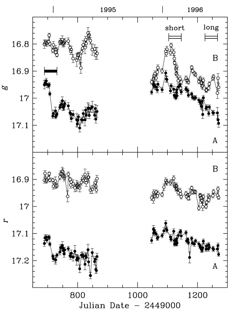
Figure 1: The 1995 and 1996 $g$ and $r$ band light curves (with 1$\sigma$ error bars) for images A (filled points) and B (open points) of the gravitationally lensed quasar 0957+561. The sharp event observed at the beginning of the 1995 season (December 94–January 95) in the $g$ light curve of the leading (A) image is marked with a horizontal bar. Based on previously reported time delays in this system, two predictions for the 1996 B light curve were presented in Paper I; they are also marked (February and June 96). The data provide compelling evidence in favor of the shorter delay, thus resolving a long-standing controversy.

Figure 1 displays our $g$ and $r$ data for images A and B in the 1995 and 1996 seasons, in other words our complete photometric data set. This data is available in the elt/:0957 subdirectory of the anonymous ftp area at astro.princeton.edu.

The predictions of the short time delay set forth in Paper I can be confirmed by inspection of Fig. 1 without need for the detailed statistical analysis presented in the next section. The sharp event which Paper I noted in the $g$ band light curve of image A in early 1995 is marked in Fig. 1, as are the times of its predicted appearance in the 1996 image B light curve. An event of just the expected amplitude and duration is seen in image B at the time corresponding to the short delay, and no such feature is seen at a time corresponding to the long delay. Although we will proceed to a quantitative analysis below, the qualitative success of the short delay prediction is compelling.

Note that Fig. 1 also displays the rather quiescent behavior of image A in 1996, which corresponds to the predicted 1997 behavior of image B, modulo the now determined delay and magnitude offset. It also emphasizes the good fortune of the occurrence of the sharp $g$ band event in image A shortly after the beginning of our monitoring program; no comparable feature has been seen since!

Also note that photometric events in the $r$ band are consistently smaller in amplitude than those in the $g$ band. Since most previous monitoring programs have concentrated their attention in red bands (probably to minimize problems with moonlight), this may explain some of the difficulty in obtaining a definitive time delay measurement.

3 The Best Fit Delay and Its Uncertainty

In this section, we present a series of statistical comparisons of our 1995 image A light curve with the 1996 image B light curve. The goals of these analyses are 1) to determine the best estimate differential time delay for 0957+561A,B; 2) to quantitatively assess its error (95% confidence interval); and 3) to demonstrate that the data provide a robust delay measurement. This last point deserves brief elaboration: Previous attempts to measure the 0957+561A,B time delay from radio and optical data have often depended as much on the statistical techniques employed as upon the data, i.e., different methods gave different answers when applied to the same data (see references in § 1). Moreover, even the best delay as determined by a single method was unstable against the inclusion or exclusion of a few data points in some cases (PHKRS). We demonstrate below that the data shown in Fig. 1 produce no such difficulties or ambiguities.

Table 1 and Fig. 2 summarize the results of our statistical comparisons of the 1995 image A light curve with the 1996 image B data. We employ four different statistical methods on four subsets of the complete data set and four parameterized models of how the image A and B light curves are related, although we do not present all 64 of the possible combinations here.

Of the at least 11 different statistical analyses previously applied to 0957+561A,B optical and radio light curves by various authors (tabulated by Haarsma et al. 1996), we have selected four representative ones intended to span the range of reasonable approaches for analysis of our data.

1. Linear method: First and simplest, each light curve and its errors are linearly interpolated, and the data points from the other light curve are shifted so as to minimize $\bar{\chi}^{2}$ ($\chi^{2}$ per degree of freedom). The number of degrees of freedom is equal to the number of overlapping data points in the shifted light curves minus the number of fitted parameters. Time delays with a small overlap of data are thus penalized with respect to delays where the overlap is significant. The 95% confidence interval quoted in Table 1 for each fitted parameter is derived by bootstrap resampling of residuals from the combined light curve smoothed by a 7-point triangular filter with a maximum length of 28 days. The confidence interval is robust with respect to the choice of the smoothing filter.

2. PRH method: As emphasized by Press et al. (1992a, b), interpolation of the light curves is a crucial ingredient in any method, and we adopt their rather elegant, though somewhat assumption laden, interpolation scheme plus $\chi^{2}$ minimization as our second method. The PRH method relies heavily on a model of the structure function of the source’s intrinsic variability. We have taken a (measured) structure function of $\log[C_{g}(\tau)]=-4.3+0.86\tau$; $\log[C_{r}(\tau)]=-4.5+0.83\tau$, where $\tau$ is in days and $C$ is in magnitudes squared. The quoted error on the PRH scaled $\chi^{2}$ method is the $\Delta\chi^{2}$ interval of $\pm 4$. While the association of a 95% (or any other specific) confidence interval with this $\Delta\chi^{2}$ interval is problematic, it provides a rough estimate of the measurement error; we refer readers to PRH for further discussion.

3. PHKRS method: As an alternative to $\chi^{2}$ minimization and as a more assumption-free approach, we adopt a non-parametric technique suggested by PHKRS as a third method. In particular, we use their dispersion measure $D_{4,k}^{2}$ from the second paper with linearly decreasing weights $S_{n,m}^{(2)}$ and decorrelation length of $\delta=7$ days. Here again 95% confidence intervals quoted in Table 1 are derived from the bootstrap resampling of residuals.

4. Cross-correlation method: Finally, we have employed a conventional cross-correlation analysis, similar to that used by Schild & Cholfin (1986), Vanderriest et al. (1989), Schild (1990), and Lehár et al. (1992), as our fourth method; this technique also requires interpolation but seems to be rather insensitive to its details. Here we report cross-correlation results using only the simplest linear interpolation scheme. The errors in Table 1 for this method are estimated 1$\sigma$ bounds on the position of the correlation peak based on a bootstrapping analysis.

The statistical methods described above have been applied to four subsets of our light curve data. First, we have considered only the $g$ band data; we believe that this gives the best and most reliable delay due to the high signal-to-noise provided by the sharp event. Second, we have treated the $r$ band data separately; it provides a partially independent, though lower signal-to-noise, delay determination. Third, we have combined the $g$ and $r$ data to find overall best fit parameter values. Fourth, we have used only the JD 2449689–2449731 interval of the 1995 image A light curve, i.e., the sharp $g$ band event alone, to search the 1996 image B light curve for a best fit. This last subsampling of the data corresponds most closely to testing the Paper I prediction and is not an a posteriori (an hence invalid) editing of the data only because of that prediction.

The simplest model of the mapping of the A image light curve into that of the B image is just a fixed offset in time, $\Delta t$, and a fixed magnitude offset, $\Delta m$. These two parameters correspond to the macrolensing differential delays and image magnifications. We also consider models in which the magnitude offset is allowed to be a linear function of time at a rate $\mu$, motivated by the possibility that one or both images are being affected by microlensing events with characteristic time scales long compared to the delay and the extent of the observed light curves (Chang & Refsdal 1979; Young 1981; Gott 1981; Falco, Wambsganss & Schneider 1991). Finally, we know that the image B photometry is contaminated by the light of the lensing galaxy G1, especially in the $r$ band due to the galaxy’s red color relative to the quasar source. Thus, we consider a parameter $m_{\rm gal}$ which represents a constant flux added to that of the source in image B. The general form of our model of the relation of the image A light curve to that of image B is, therefore

$$10^{-0.4m_{B}(t)}=10^{-0.4\left[m_{A}(t-\Delta t)+\Delta m+\mu(t-t_{0})\right]}+10^{-0.4m_{\rm gal}}\quad,$$ (1)

where $m_{A}$, $m_{B}$ are the measured image A and B magnitudes; $\Delta t$ is the time delay; $\Delta m$, $\mu$ are the magnitude offset and its rate of change; $t_{0}$ = JD 2450000 (arbitrarily chosen); and $m_{\rm gal}$ is the magnitude of the lensing galaxy G1 which contaminates image B photometry. As shown in Table 1, we have experimented with models in which up to three parameters are allowed to vary as well as ones in which the less interesting ones, $\mu$ and $m_{\rm gal}$ are neglected, that is fixed at zero and infinity, respectively.

Table 1 shows the results of a selected set of combinations of our statistical methods, light curve mapping models and versions of the data. All 64 possible combinations are not shown for the sake of clarity and because some of the statistical methods and some versions of the data do not lend themselves well to the determination of some parameters. However, we emphasize that we are aware of no combination of method, data subset and model which gives a $\Delta t$ value significantly different from those shown in Table 1. Fig. 2 displays the variation of the minimized statistical parameter with respect to $\Delta t$ for the $g$ band light curves with each of our four methods. In this figure microlensing and galaxy terms are not included in the fits.

The most important conclusion to be drawn from Table 1 and Fig. 2 is that the best fit value of $\Delta t$ is extremely robust, changing by less than 1% whatever method, data version or parameterized model is used. The delay error estimates produced by the various statistical analyses are somewhat more varied, with those methods that assume greater knowledge of the statistical character of the light curves naturally producing smaller error estimates, but in no case is the estimated error greater than 3%. As we shall see in the next section, the error in the measured delay now contributes negligibly to the error in the deduced global value of $H_{0}$.

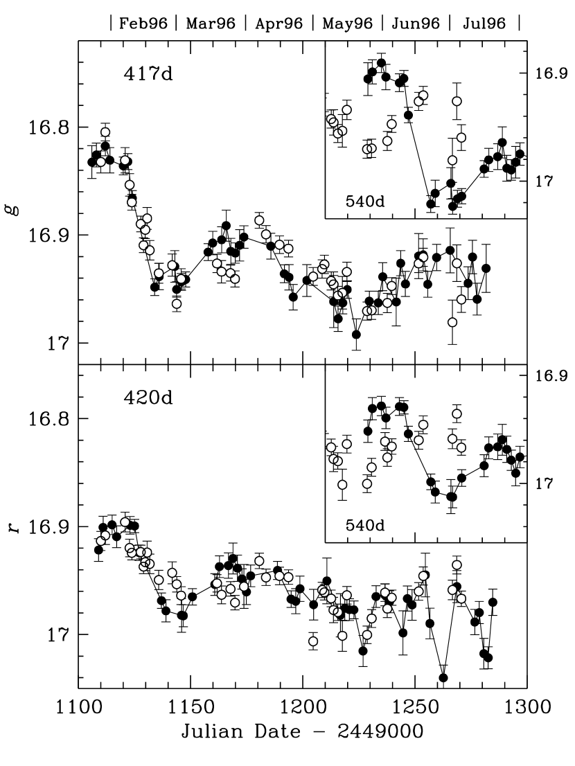
Figure 3: The 1995 A light curves (filled points) shifted by the optimal values of the time delay $\Delta t$ and the magnitude offset $\Delta m$, superimposed on the 1996 image B data (open points). The fits are based on the linear method analysis, but the parameters given by other fitting methods are nearly identical. See the text for details. Insets show the overlapping regions of A and B light curves assuming the long delay of 540 days (and fitting for the magnitude offset). This delay is clearly excluded by the data.

Because it is simple and seems to work as well as any other approach for this data set, we adopt the results of the linear method applied to the $g$ band light curves with just a $\Delta t,\Delta m$ model as our final numbers. This gives a delay of $417\pm 3$ days and a $g$ band magnitude offset of $-118^{+6}_{-8}$ millimag (B is brighter than A). Fig. 3 displays this fit and the corresponding independent fit (420 days, $-215$ millimag) for the $r$ band data; it also shows the cleanly rejected fit which corresponds to the long delay of about 540 days in the figure insets.

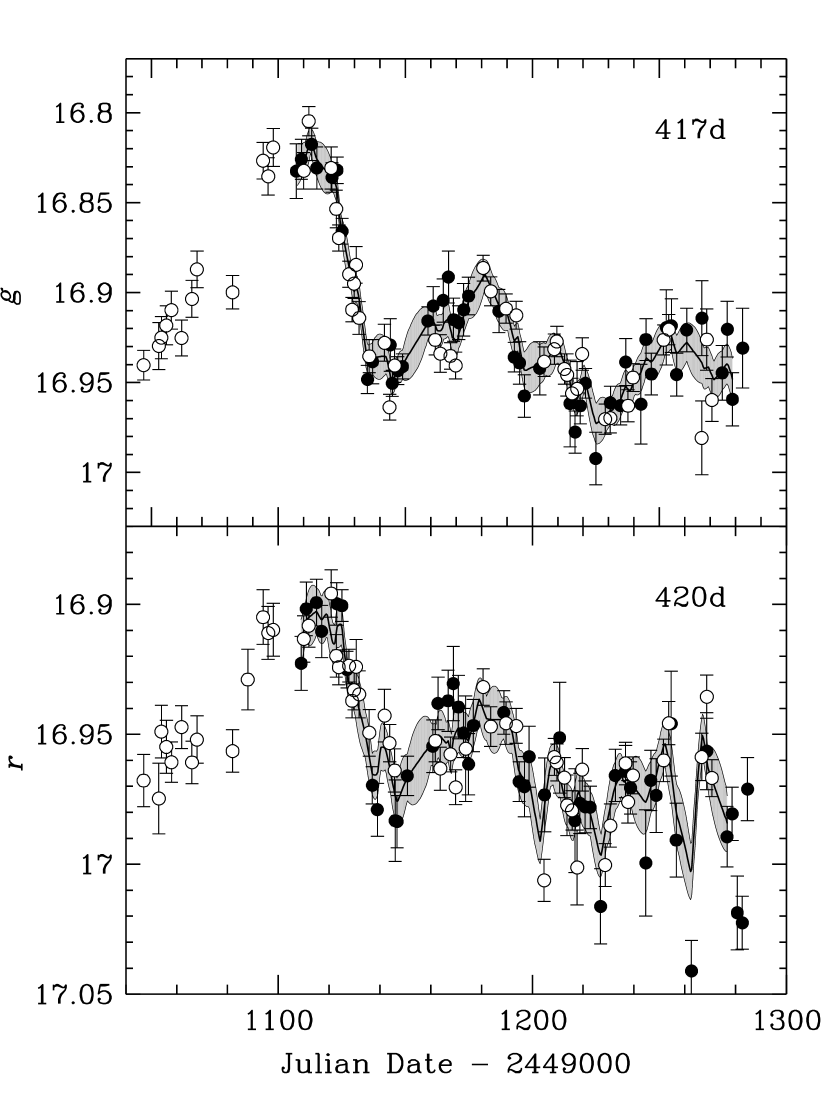
Figure 4: The optimal PRH reconstruction of the shifted and combined A (filled points) and B (open points) light curves of 0957+561. The shaded region (“snake”) corresponds to the 1$\sigma$ confidence interval of the reconstruction. The error bars are the photometric 1$\sigma$ measurement errors.

In addition to providing best fits and error estimates, the PRH method produces an optimal (under the assumed statistical properties of the source light curve) reconstruction of the underlying single light curve sampled in the two images, and a “snake” corresponding to its uncertainty at each point. This reconstruction and its comparison to the data are shown in Fig. 4.

4 A Measurement of the Global Value of $H_{0}$

For a complex gravitational lens system such as 0957+561, reliable measurement of the differential time delay may still leave one far from the goal of a good measurement of $H_{0}$ (e.g., Schechter et al. 1996), simply because of uncertainties in the lens mass distribution and its implied conversion factor between $c\Delta t$ and the source angular diameter distance (Falco, Gorenstein & Shapiro 1991; Kochanek 1991). This was once a major obstacle, but fortunately an extensive recent theoretical modeling study of 0957+561 by GN appears to have resolved the major ambiguities with the exception of one effect noted by Falco, Gorenstein & Shapiro (1985); and Gorenstein, Falco & Shapiro (1988); see below. In particular, GN use 15 known observables to constrain a set of lens mass models having 9 free parameters. The relation between time delay and distance is controlled primarily by the total projected mass of the lens within the circle defined by the diameter connecting the two source images $M(<r)$ and by its derivative $dM/dr$ (Chang & Refsdal 1976; Refsdal 1992; Wambsganss & Paczyński 1994). GN find that the observed image separation $\Delta\theta=6.1\arcsec$ and the observed mapping of the complex 5-component structure in the VLBI images of the image A and B (Garrett et al. 1994) nearly fix $M(<r)$ and $dM/dr$ at the image positions, respectively, independent of other features of the lens model. For example, compared to their best fit model (which models G1 as a softened power-law sphere), GN find that the best-fit King model (after Falco et al. 1991) with a compact nucleus gives only a 3% higher value of $H_{0}$ despite introducing a central black hole in G1 with a mass of $2.5\times 10^{10}M_{\odot}$. Including ellipticity in G1 at the observed value of $\epsilon=0.3$ and major axis position angle of $55\arcdeg$ (Bernstein, Tyson & Kochanek 1993) increases $H_{0}$ by 2%. Adding perturbations from the two closest cluster galaxies reduces it by 4%. Moreover, changing $\Omega_{0}$ from unity, the value otherwise assumed throughout this paper, to 0.1 increases $H_{0}$ by only 7%. Introducing the cosmological constant while keeping the universe flat results in an increase of just 4% in the $\Omega_{0}=0.25$, $\Omega_{\Lambda}=0.75$ model.

Unfortunately, the distance conversion factor supplied by the GN models remains quite sensitive to one remaining degeneracy which cannot be removed by the observed properties of the lensing event itself (Falco et al. 1985, Gorenstein et al. 1988), namely how much of the lensing is contributed by mass associated with the galaxy G1 versus how much is supplied by the associated and superimposed galaxy cluster. Since these two must sum to a known value (in order to produce the observed splitting), the degeneracy may be parameterized by either the one or the other. GN adopt $\sigma_{\rm obs}$, the central line-of-sight velocity dispersion of G1, to measure its contribution and $\kappa$, the dimensionless lensing convergence contributed by the cluster, to parameterize its effect. In order to derive an $H_{0}$ value, we need to independently measure one or the other parameter. Measuring both provides an internal consistency check.

Fischer et al. (1996) have recently reported a mapping of the cluster mass distribution based on the observed distortion of faint background galaxies, a technique which is now well developed and has been successfully applied to several other galaxy clusters (e.g. Tyson, Valdes & Wenk 1990; Tyson & Fischer 1995; Squires et al. 1996a, b). Unfortunately, the mass profile reported by Fischer et al. is centered on G1, rather than the center of mass in the field located some $22\arcsec$ northeast. Since the distortion of background galaxies at the two quasar image positions is dominated by the mass of G1, it is difficult to independently estimate the contribution of the cluster. This would have been possible if the cluster profile had been extracted around its observed center and the region around G1 excluded from the weak lensing analysis. Assuming circular symmetry, one could have then estimated $\kappa$ at the radius corresponding to G1 from the uncontaminated area in the cluster.

One can still make an indirect estimate of $\kappa$ from the total mass of the cluster, its core radius and the location of G1 with respect to the cluster center. Following GN and Kochanek (1991), we assume that the cluster potential corresponds to a softened isothermal sphere $\phi(r)=b_{\rm crit}(r^{2}+r_{c}^{2})^{1/2}$, where $r_{c}$ is the core radius and $b_{\rm crit}=17\arcsec.3(\sigma_{\rm cl}/1000\,{\rm km\,s^{-1}})^{2}$ is the critical radius of the cluster expressed in terms of its velocity dispersion $\sigma_{\rm cl}$. This potential results in a density profile slightly different from that of Fischer et al. (1996), but well within their observational uncertainty. The local convergence at a position $r$ in the cluster is then given by $\kappa=\frac{1}{2}b_{\rm crit}(r^{2}+2r_{c}^{2})/(r^{2}+r_{c}^{2})^{3/2}$. Using direct spectroscopy of cluster galaxies, Angonin-Willaime, Soucail & Vanderriest (1994) find $\sigma_{\rm cl}=714\pm 130$ km/s. The cluster mass estimate from weak lensing, $M(r<1\,{\rm Mpc})=3.9\pm 1.2\times 10^{14}M_{\odot}$ (Fischer et al. 1996), implies a slightly higher velocity dispersion of $\sigma_{\rm cl}=730\pm 120$ km/s. We thus adopt $\sigma_{\rm cl}=720\pm 250$ km/s as our 95% confidence region. Using $r=22\arcsec$ for the distance of G1 from the center of the cluster and $r_{c}=5\arcsec$ for the cluster core radius (as measured by Fischer et al.), our final estimate for the cluster surface density at the position of the lensing event is $\kappa=0.22\pm 0.14$ (2$\sigma$). This result is insensitive to the precise value of $r_{c}$, but it could increase considerably if G1 were much closer to the center of the cluster. At that point, however, the quadratic approximation of the cluster potential (which only includes the convergence and shear) would break down as well.

Thus, including first only the quoted errors in the GN model and those of our time delay and then adding the dominant contribution from the $\kappa$ uncertainty, we find

$$H_{0}=64^{+4.5}_{-5.3}\;\left(\frac{1-\kappa}{0.78}\right)\;{\rm km\,s^{-1}\,Mpc^{-1}}=64^{+12}_{-13}\;{\rm km\,s^{-1}\,Mpc^{-1}}$$ (2)

where the errors reflect the total 95% confidence interval. The primary remaining systematic uncertainty in this calculation is associated with the mean redshift of the background galaxy population used to map the cluster mass distribution, somewhat arbitrarily assumed to be 1.2 by Fischer et al. (1996). If it were allowed to vary between 0.75 and 3, the derived value of $H_{0}$ would range between 58 and 68 km/s/Mpc, respectively. Considering very extreme possibilities, $H_{0}$ would vary from 37 to 70 km/s/Mpc for mean background galaxy redshifts between 0.5 and infinity.

Falco et al. (1997, as quoted by M. Davis 1996, private communication) recently obtained a new measurement of the velocity dispersion in G1 from a high signal-to-noise Keck LRIS spectrum. Although there are some puzzling features of their data, a surprisingly rapid variation in $\sigma_{\rm obs}$ along the slit in particular, they obtain a value roughly in the range $\sigma_{\rm obs}=275\pm 30$ km/s (2$\sigma$). This is much more accurate than—but consistent with—the only previously reported value of $303\pm 50$ km/s (Rhee 1991), which was based on a significantly lower signal-to-noise spectrum. Inserting this new value of $\sigma_{\rm obs}$ and again propagating all the relevant errors, we find

$$H_{0}=64^{+7.5}_{-9.8}\;\left(\frac{\sigma_{\rm obs}}{275\;{\rm km\,s^{-1}}}\right)^{2}\;{\rm km\,s^{-1}\,Mpc^{-1}}=64^{+13}_{-14}\;{\rm km\,s^{-1}\,Mpc^{-1}}\quad.$$ (3)

where we again quote 2$\sigma$ error intervals. The GN model error, included in our $H_{0}$ uncertainty, allows for finite aperture effects and possible anisotropy of stellar orbits.

It is important and reassuring that these two entirely independent methods of resolving the galaxy-cluster degeneracy in 0957+561 give very similar and entirely consistent results. For example, if one assumes an extremely low value of 0.5 for the mean redshift of background galaxies in the $\kappa$ method, this would yield a very small value of $H_{0}$ (see above), but would also contradict the Falco et al. (1996) result by implying a G1 velocity dispersion of only 210 km/s.

We cannot properly average (2) and (3) since they are based on the same lens mass model (i.e., are not entirely independent), but they can be approximately summarized by $H_{0}=64\pm 13$ km/s/Mpc at 95% confidence, or $\pm$ 10% at 1$\sigma$.

5 Summary and Discussion

Our main results may be summarized as follows: The sharp photometric event predicted in the 1996 0957+561B light curve in Paper I based on the observed 1995 image A light curve has been observed at the time corresponding to the so called short (about 420 day) delay, thus confirming its validity. No such event was observed at a time corresponding to the long (540 day) delay, thus rejecting it. The time delay determined by the data presented here and in Paper I is quite robust and has a best fit value of $417\pm 3$ days. Combining this value with the latest theoretical models of the lens mass distribution plus two independent measurements of the relative contributions of the galaxy G1 and the associated galaxy cluster indicates that the global value of $H_{0}$ lies in the interval 51 to 77 km/s/Mpc with a most probable value in the range 58–70 km/s/Mpc. Although the possibility of significant systematic error remains, especially in the lens mass distribution model, this result is likely as accurate and reliable as the best conventional measures of $H_{0}$.

Though still a significant potential source of systematic error, there is reason to believe that further refinements of the lens mass distribution model will have little effect on the derived value of $H_{0}$, as argued in detail at the beginning of § 4, following GN. The point is that the constraints provided by the detailed matching of the A and B VLBI images (Garrett et al. 1994) appear to sufficiently constrain the critical physical properties of lens models, particularly the gradient of the projected lens mass distribution at the image positions, that even models which differ substantially in their other properties will yield nearly the same value of $H_{0}$ (Chang & Refsdal 1976; Refsdal 1992; Wambsganss & Paczyński 1994). These critical VLBI constraints were not available to earlier modelers, e.g., Falco et al. (1991), who derived values of $H_{0}$ varying from the GN results by up to 50% for a fixed delay and G1 velocity dispersion. Of course, further exploration of the space of all possible lensing models of 0957+561A,B will be useful to determine just how much the derived $H_{0}$ value can be changed within the constraints of the VLBI maps; the extensive modeling by GN was not exhaustive of all possibilities.

The data presented here have some interesting implications beyond those for the extragalactic distance scale. We now turn briefly to these.

First, note in Figures 3 and 4 that the time shifted and magnitude offset light curves of images A and B do not appear to match perfectly, even though they are strikingly similar. In particular, the image B points fall a few hundredths of a magnitude below (fainter than) those of the shifted and offset image A data during the interval JD 2450160 to 2450175 and then even more slightly above them during 2450175 to 2450220. We have made no test of the statistical significance of this discrepancy, but no acceptable delay and offset removes it, nor have we been able to identify any plausible shortcoming or anomaly in the data for either image during the intervals in question which might be blamed for a spurious effect. It is tempting to speculatively attribute the mismatch to microlensing perturbations of the macrolensing event since one expects a substantial microlensing optical depth for at least image B and since claims of such effects have been made before based on earlier light curve data (Schild & Smith 1991, Schild & Thomson 1995, Schild 1996). The timescale of the mismatch (tens of days) is far shorter than that expected for strong microlensing perturbations by roughly stellar mass objects, or even massive planets, in the low optical depth limit (years to decades, Young 1981, Gott 1981), but these are not large amplitude events and the low optical depth limit probably does not apply. The small magnitude of these short time scale mismatches and the null detection of a slow offset drift $\mu$, see Table 1, may be more conservatively interpreted as upper limits on microlensing effects in the present data. We may return to this issue in a separate paper. In any case, these minor and marginally detected features do not appear to compromise or complicate the time delay measurement.

Second, the shifted and offset light curves of images A and B combine to give an intriguing record of the quasar source’s intrinsic variability, possible small microlensing perturbations aside. See Figures 3 and 4. Such data may contain important clues to the quasar’s detailed internal physics, the functioning of its accretion disk in the conventional AGN model. Although we have not yet carried out any such analyses, it is apparent that one might ask many interesting statistical question of this and similar quasar light curves.

Third, Peebles et al. (1991) and Dar (1991) point out that gravitational lensing events confirm that high-redshift galaxies and quasars are at cosmological distances. The precise repetition of the 1995 image A light curve by image B in 1996 (to roughly 1% accuracy) based on an a priori prediction provides the best such available case. It both unambiguously proves that 0957+561A,B is a bona fide case of gravitational lensing and gives an order-of-magnitude, model-independent measure of the source distance $\sim(4c\Delta t)/(\Delta\theta^{2})=1.6$ Gpc.

Turning finally to a more general perspective, 0957+561A,B appears to have provided a first and so far best success for Refsdal’s method of measuring $H_{0}$, but it is clear that there are good prospects of both improving its accuracy and extending its applications to other gravitational lens systems. Towards the former goal, improved measurements of G1’s position and velocity dispersion $\sigma_{\rm obs}$ and of the galaxy cluster’s mass distribution are clearly possible; some are already underway. Direct measurement of redshifts of the distorted background galaxy images will be challenging but would remove a major systematic uncertainty. Further theoretical exploration of the lens mass model space is also desirable to verify the uniqueness of the GN model. Rapid progress can also be expected using other lens systems. Recently, Schechter et al. (1996) have reported a convincing, though only moderately accurate, pair of time delays in the 1115+080A,B,C system. The accuracy can almost certainly be improved. It remains to be seen whether or not sufficiently unique and well constrained models of this system can be obtained to allow useful $H_{0}$ measurements. Systems such as B0218+357, for which a very rough estimate of the delay has been obtained from radio polarimetry (Corbett et al. 1996) should be powerful for distance determinations because their resolved structure provides strong model constraints. The rate of discovery of new lens systems is likely to increase, so we may expect yet more suitable “Rosetta Stone” systems to be found in the future.

As noted in § 1, no known or imagined effect or systematic error would cause different lens systems to give the same wrong answer consistently. Thus, if good time delay measurements and well constrained lens models yield the same value of $H_{0}$ for a few different lens systems (with different angular sizes, lens and source redshift, et cetera), the problem of measuring the global value of Hubble’s constant will have been effectively solved.

TABLE 1

method	band	fitted parameters	$\Delta t$	$\Delta m$	$\mu$	$m_{\rm gal}$
			[day]	[millimag]	[$\mu$mag/day]	[mag]
Linear	$g$	$\Delta t$, $\Delta m$	$417^{+3}_{-3}$	$-118^{+6}_{-8}$
		$\Delta t$, $\Delta m$, $\mu$	$417^{+5}_{-4}$	$-118^{+31}_{-27}$	$-4^{+132}_{-153}$
		$\Delta t$, $\Delta m$, $m_{\rm gal}$	$417^{+4}_{-4}$	$-119^{+116}_{-7}$		$>19.4$
Linear (event)	$g$	$\Delta t$, $\Delta m$	$417^{+3}_{-4}$	$-123^{+13}_{-12}$
Linear	$r$	$\Delta t$, $\Delta m$	$420^{+6}_{-9}$	$-215^{+6}_{-8}$
		$\Delta t$, $\Delta m$, $\mu$	$420^{+8}_{-8}$	$-200^{+35}_{-27}$	$-87^{+131}_{-188}$
		$\Delta t$, $\Delta m$, $m_{\rm gal}$	$420^{+7}_{-9}$	$-215^{+89}_{-9}$		$>19.7$
Linear	$gr$	$\Delta t$, $\Delta m$	$418^{+4}_{-2}$
PRH	$g$	$\Delta t$, $\Delta m$	$417^{+1}_{-1}$	$-117^{+6}_{-6}$
		$\Delta t$, $\Delta m$, $\mu$	$417$	$-117$	$-39$
		$\Delta t$, $\Delta m$, $m_{\rm gal}$	$417$	$-126$		$29.4$
PRH	$r$	$\Delta t$, $\Delta m$	$420^{+2}_{-1}$	$-215^{+6}_{-4}$
		$\Delta t$, $\Delta m$, $\mu$	$420$	$-245$	$-127$
		$\Delta t$, $\Delta m$, $m_{\rm gal}$	$420$	$-214$		$29.2$
PHKRS	$g$	$\Delta t$, $\Delta m$	$417^{+2}_{-4}$	$-117^{+5}_{-10}$
	$r$	$\Delta t$, $\Delta m$	$419^{+9}_{-9}$	$-212^{+7}_{-12}$
	$gr$	$\Delta t$, $\Delta m$	$417^{+4}_{-4}$
Cross-correlation	$g$	$\Delta t$	$420^{+4}_{-4}$
	$r$	$\Delta t$	$422^{+8}_{-8}$

Figure 2: Figure of merit for various statistical methods as a function of time delay $\Delta t$ based on $g$ band light curves. Curves are arranged so that their minima correspond to the best fit delays. The second fitted parameter, magnitude offset $\Delta m$, was minimized at each value of $\Delta t$. The values of $\bar{\chi}^{2}$ for the linear and PRH methods are represented with solid and dot-dash lines respectively; the dispersion measure $D^{2}$ of the PHKRS method is dashed, and the complement of the cross-correlation coefficient is dotted. Note that three different vertical coordinates are represented, depending on the statistical technique. All methods give minima at $\sim$ 417–420 days and strongly reject a delay of $\sim$ 540 days.

References

- (1)
- (2) Angonin-Willaime, M.-C., Soucail, G., & Vanderriest, C. 1994, A&A, 291, 411
- (3)
- (4) Bernstein, G. M., Tyson, J. A., & Kochanek, C. S. 1993, AJ, 105, 816
- (5)
- (6) Beskin, G. M., & Oknyanskij V. L. 1995, A&A, 304, 341
- (7)
- (8) Blandford, R.D., & Narayan, R. 1992, ARA&A, 30, 311
- (9)
- (10) Chang, K., & Refsdal, S. 1976, International CNRS Coll., 263, 369
- (11)
- (12) Chang, K., & Refsdal, S. 1979, Nature, 282, 561
- (13)
- (14) Corbett, E. A., Browne, I. W. A., Wilkinson, P. N., & Patnaik, A. R. 1996, in Astrophysical Applications of Gravitational Lensing, ed. C. S. Kochanek, & J. N. Hewitt (Dodrecht: Kluwer), 37
- (15)
- (16) Dar, A. 1991, ApJ, 382, L1
- (17)
- (18) Falco, E. E., Gorenstein, M. V., & Shapiro, I. I. 1985, ApJ, 289, L1
- (19)
- (20) Falco, E. E., Gorenstein, M. V., & Shapiro, I. I. 1991, ApJ, 372, 364
- (21)
- (22) Falco, E. E., Wambsganss, J., & Schneider, P. 1991, MNRAS, 251, 698
- (23)
- (24) Fischer, P., Bernstein, G., Rhee, G., & Tyson, J. A. 1996, AJ, in press (astro-ph/9608117)
- (25)
- (26) Florentin-Nielsen, R. 1984, A&A, 138, L19
- (27)
- (28) Garrett, M. A., Calder, R. J., Porcas, R. W., King, L. J., Walsh, D., & Wilkinson, P. N. 1994, MNRAS, 270, 457
- (29)
- (30) Gorenstein, M. V., Falco, E. E., & Shapiro, I. I. 1988, ApJ, 327, 693
- (31)
- (32) Gott, J. R. 1981, ApJ, 243, 140
- (33)
- (34) Grogin, N. A., & Narayan, R. 1996, ApJ, 464, 92 & 473, 570 (GN)
- (35)
- (36) Haarsma, D. B., Hewitt, J. N., Lehár, J., & Burke, B. F. 1996, ApJ, submitted (astro-ph/9607080)
- (37)
- (38) Keel, W. C. 1982, ApJ, 255, 20
- (39)
- (40) Kochanek, C. S. 1991, ApJ, 382, 58
- (41)
- (42) Kundić, T., Colley, W. N., Gott, J. R. III, Malhotra, S., Pen, U., Rhoads, J. E., Stanek, K. Z., & Turner, E. L. 1995, ApJ, 455, L5 (Paper I)
- (43)
- (44) Lehár, J., Hewitt, J. N., Roberts, D. H., & Burke, B. F. 1992, ApJ, 384, 453
- (45)
- (46) Lloyd, C. 1981, Nature, 294, 727
- (47)
- (48) Narasimha, D., Subramanian, K., & Chitre, S. M. 1984, MNRAS, 210, 79
- (49)
- (50) Narayan, R. 1991, ApJ, 378, L5
- (51)
- (52) Narayan, R. & Bartelmann M. 1996, astro-ph/9606001
- (53)
- (54) Oscoz, A., Serra-Ricart, M., Goicoechea, L. J., Buitrago, J., & Mediavilla, E. 1996, ApJ, 470, L19
- (55)
- (56) Peebles, P. J. E., Schramm, D. N., Turner, E. L., & Kron, R. G. 1991, Nature, 352, 769
- (57)
- (58) Pelt, J., Hoff, W., Kayser, R., Refsdal, S., & Schramm, T. 1994, A&A, 286, 775 (PHKRS)
- (59)
- (60) Pelt, J., Kayser, R., Refsdal, S., & Schramm, T. 1996, A&A, 305, 97 (PHKRS)
- (61)
- (62) Press, W. H., Rybicki, G. B., & Hewitt, J. N. 1992a, ApJ, 385, 404 (PRH)
- (63)
- (64) Press, W. H., Rybicki, G. B., & Hewitt, J. N. 1992b, ApJ, 385, 416 (PRH)
- (65)
- (66) Refsdal, S. 1964, MNRAS, 128, 307
- (67)
- (68) Refsdal, S. 1966, MNRAS, 132, 101
- (69)
- (70) Refsdal, S. 1992, in Gravitational Lenses, eds. R. Kayser, T. Schramm, & L. Nieser, Hamburg: Springer Verlag, 61
- (71)
- (72) Rhee, G. 1991, Nature, 350, 211
- (73)
- (74) Schechter, P. L. et al. 1996, ApJ, submitted
- (75)
- (76) Schild, R. E. 1990, AJ, 100, 1771
- (77)
- (78) Schild, R. E. 1996, ApJ, 464, 125
- (79)
- (80) Schild, R. E., & Cholfin, B. 1986, ApJ, 300, 209
- (81)
- (82) Schild, R. E., & Smith, R. C. 1991, AJ, 101, 813
- (83)
- (84) Schild, R., & Thomson, D. J. 1995, AJ, 109, 1970
- (85)
- (86) Squires, G., Kaiser, N., Babul, A., Fahlman, G., Woods, D., Neumann, D. M., Böhringer, H. 1996a, ApJ, 461, 572
- (87)
- (88) Squires, G., Kaiser, N., Fahlman, G., Babul, A., Woods, D., 1996b, ApJ, 469, 73
- (89)
- (90) Turner, E. L., Cen, R., & Ostriker, J. P. 1992, AJ, 103, 1427
- (91)
- (92) Tyson, J. A., Valdes, F., & Wenk, R. A. 1990, ApJ, 349, L1
- (93)
- (94) Tyson, J. A., & Fischer, P. 1995, ApJ, 446, L55
- (95)
- (96) Vanderriest, C., Schneider, J., Herpe, G., Chevreton, M., Moles, M., & Wlérick, G. 1989, A&A, 215, 1
- (97)
- (98) Walsh, D., Carswell, R. F. & Weymann, R. J. 1979, Nature, 279, 381
- (99)
- (100) Wambsganss, J., & Paczyński, B. 1994, AJ, 108, 1156
- (101)
- (102) Young, P. 1981, ApJ, 244, 756
- (103)
- (104) Young, P., Gunn, J. E., Kristian, J., Oke, J. B., & Westphal, J. A. 1981, ApJ, 244, 736
- (105)