THE V R I COLOURS OF HII GALAXIES

Abstract

We present a high spatial resolution CCD surface photometry study in the optical V, R and I broadband filters of a sample of 15 HII galaxies. Narrow band imaging has allowed the separation of the emission line region from the extended parts of the galaxy. The latter are assumed to represent the underlying galaxy in HII galaxies, thus, the colours of the underlying galaxy are measured. The colours of the underlying stellar continuum within the starburst are also derived by subtracting the contribution of the emission lines falling in the broad band filters. The distribution of colours of the underlying galaxy in HII galaxies is similar to the colours of other late type low surface brightness galaxies which suggests a close kinship of these with the quiescent phases of HII galaxies. However, comparison with recent evolutionary population synthesis models shows that the observational errors and the uncertainties in the models are still too large to put strict constraints on their past star formation history.

Our analysis of the morphology and structural properties, from contour maps and luminosity profiles, of this sample of 15 HII galaxies agree to what has been found in Telles (1995) and Telles, Melnick & Terlevich (1996), namely that, HII galaxies comprise two broad classes segregated by their luminosity; Type I HII galaxies are luminous and have disturbed and irregular outer shapes while Type II HII galaxies are less luminous and have regular shapes. The outer parts of their profiles are well represented by an exponential as in other types of known dwarf galaxy.

1 Introduction

The question of whether HII galaxies are primordial galaxies experiencing their very first burst of star formation or if an older stellar population from an earlier event of star formation is present has not, since it was first posed by Sargent & Searle (1970), been answered. Multi-colour surface photometry can provide with the answers. To infer ages and mix of stellar populations of HII galaxies through broad band observations one can compare the observed colours with those derived from evolutionary synthesis models. When dealing with systems with intense gaseous emission though, line emission can be a significant contributor to the total fluxes of the starburst within the corresponding broad band filters (Huchra 1977; Salzer, MacAlpine & Boroson 1989). In this case, two approaches may be considered. On one hand, one may compare the integrated colours of the starburst with synthesis models which take into account the gaseous line emission (Huchra 1977) or use stellar evolutionary models by comparing with the starburst stellar continuum alone. The latter can be derived by accounting for the contribution of the emission lines in the broad band filters of interest. We have chosen the second approach relying on the spectrophotometric information from The Spectrophotometric Catalogue of HII Galaxies (Terlevich et al. 1991, hereafter SCHG) and some assumption about the gas emission line surface distribution and the availability of state of the art stellar evolutionary population synthesis models.

In this paper, we compare the results of high spatial resolution CCD broadband optical photometry with the observed colours of samples of dwarf galaxies and with recent models of evolutionary synthesis from the literature. In the case of the starburst region in HII galaxies the combined effect of low mass stars, if present from previous episodes of star formation, on the optical colours is expected to be negligible relative to the dominant contribution of the high mass stars responsible for the observed ionized spectrum. A positive direct detection of an older stellar population in the burst region is a very difficult task. We take advantage of the high spatial resolution observations that allow us to estimate the colours beyond the line emitting regions which we will call extensions. The extensions are virtually free from line emission, therefore the light in these regions is assumed to be produced by a population of stars other than that embedded in the starburst. Thus, we put constraints on the ages of the underlying galaxy by comparing the colours of these extensions with the models and with control samples of real galaxies.

Through the means of surface photometry (e.g. morphology, structure, luminosity profiles and colours) we re-address the question of what HII galaxies resemble in their quiescent period and their possible kinship with other known types of dwarf galaxies.

We present the sample selection in Section 2, observations and data reduction in Section 3. Section 4 shows all the results of the surface photometry. In § 5 we discuss various topics raised by our data. Finally, in Section 6, we present our conclusions.

2 The Sample

Table 1: Positions and basic spectroscopic data for the galaxy sample. The data are from SCHG and from Melnick, Terlevich & Moles (1988). Oxygen abundance determinations are from: ^† Melnick, Terlevich & Moles (1988); ^‡ Telles (1995) using procedure as in Pagel et al. (1992); ^∐ R₂₃ empirical calibration from McGaugh (1991); ^∗ González-Delgado et al. (1995).

name	R.A.(1950)	$\delta$ (1950)	z	$\sigma$	${\cal F}(H\beta)$	C$(H\beta)$	W$(H\beta)$	O/H
UM 238	00 22 06.0	01 27 36	0.014		0.08	0.00	149	8.14‡
UM 133	01 42 08.0	04 38 48	0.009	17.2	0.32	0.43	65	7.69‡
UM 408	02 08 48.0	02 06 36	0.012		0.07	0.62	52	7.66‡
II Zw 40	05 53 00.6	03 24 00	0.003	35.2	1.90	1.00	170	8.13†
C0840+1044	08 39 53.2	10 44 02	0.012	34.0	0.10	0.38	55
C0840+1201	08 39 36.3	12 00 49	0.030	36.5	0.48	0.52	105	7.88†
C08-28A	08 42 45.4	16 16 46	0.054	49.1	0.28	0.77	35	8.40∐
Mrk 36	11 02 01.2	29 24 00	0.002	16.0	1.40	0.70	70	7.86†
UM 448	11 39 38.3	00 36 38	0.018	40.8	2.20	0.48	45	8.03‡
UM 455	11 47 50.0	-00 15 01	0.012	20.6	0.09	0.26	55	7.84†
UM 461A	11 48 59.4	-02 05 41	0.005	14.5	0.70	0.40	155	7.74†
UM 483	12 09 41.0	00 21 00	0.007		0.14	0.11	26	8.24‡
C1212+1148	12 10 56.5	11 57 36	0.023	34.2	0.13	0.63	60	7.98∐
C1409+1200	14 09 14.3	11 59 33	0.056	52.3	0.19	0.44	130	8.18†
UM 167	23 33 40.0	01 52 30	0.009		2.51	0.26	28	8.50∗

The sample we selected for the surface photometry study is a sub-sample of SCHG for which emission line width measurements are, in most cases, available in the literature (Melnick, Terlevich & Moles 1988). A recent review of the spectroscopic properties of the HII galaxies in SCHG is given by Telles (1995, and references therein). We have compiled in Table 1 some of the basic spectroscopic data of the present galaxy sample. Column 1 gives the name of the objects used in this study, while columns 2 and 3 give their 1950 position. Column 4 gives the redshift (z) and 5 gives the emission line width ($\sigma$) in  $\hbox{km}\thinspace\hbox{s}^{-1}$, as given by Melnick, Terlevich & Moles (1988). Column 6 gives the Flux in H$\beta$ [${\cal F}(H\beta)$] in units of 10^-13  erg $\hbox{cm}^{2}$ s^-1, 7 gives the observed reddening coefficient C$(H\beta)$ obtained from the Balmer decrement and column 8 the equivalent width of H$\beta$ [W$(H\beta)$] in Å. The last column gives the oxygen abundance in the units of 12+log(O/H). Whenever we did not find in the literature, we calculated the oxygen abundances using the prescriptions given in Pagel et al. (1992) in case the [OIII] $\lambda 4363$ line was detected. Otherwise, we have used the empirical abundance estimator devised by Pagel et al. (1979) with the calibration of McGaugh (1991).

3 Observations and Data Reduction

Table 2: Journal of Observations.

name	instrument	date	CCD	pixel	Exposure time
				size ($\,{}^{\prime\prime}$)	V	R	I
UM 238	NOT2.5m	13JAN91	TK512-011	0.20	1000	1000	1200
UM 448	NOT2.5m	13JAN91	TK512-011	0.20	1000	1000	1000
II Zw 40	NOT2.5m	13JAN91	TK512-011	0.20	1000	1000	500+500
C08-28A	NOT2.5m	14JAN91	TK512-011	0.20	1000	1000	1000
Mrk 36	NOT2.5m	14JAN91	TK512-011	0.20	1000	1000	1000
UM 455	NOT2.5m	14JAN91	TK512-011	0.20	1000	1000
UM 133	NOT2.5m	15JAN91	TK512-011	0.20	1000	1000	1000
UM 408	NOT2.5m	15JAN91	TK512-011	0.20	1000	1000	1000
C0840+1044	NOT2.5m	15JAN91	TK512-011	0.20	1000	1000	1000
UM 461	NOT2.5m	15JAN91	TK512-011	0.20	1000	1000	1000
C1212+1148	NOT2.5m	15JAN91	TK512-011	0.20	500	500	500
C0840+1201	JKT1.0m	11MAR92	GEC3	0.33	1800	1800	1200+1200
UM 483	JKT1.0m	11MAR92	GEC3	0.33	1800	1800	1800
C1409+1200	JKT1.0m	11MAR92	GEC3	0.33	1800	1800	1800+1800
UM 167	JKT1.0m	25OCT92	EEV7	0.31	500+300+200	200	1800

The observations were made using the 2.5-m Nordic Optical Telescope (NOT) and the 1.0-m the Jacobus Kapteyn Telescope (JKT) at the Observatorio del Roque de Los Muchachos, La Palma, Canary Islands. The journal of all broadband observations is given in Table 2. The JKT observations were obtained as part of the GEFE project. The nights were photometric and had typically sub-arcsecond seeing conditions. For the NOT observations the combined optical system at the Cassegrain focal station gives a focal ratio of f/11.0. We have used a Tektronix TK512-011  “thick ” frontside-illuminated 512x512 CCD chip giving a total field of about $1.7{\tt{}^{\prime}}\times 1.7{\tt{}^{\prime}}$. Small correction for non-linearity of this CCD chip had to be applied which should not introduce any significant error to the photometry. We used the linearity curve determined by Hans Kjeldsen (private communication) to perform this correction. For the JKT observations in March 91 we used the GEC3 400x590 CCD chip which gives a total field of $2.2{\tt{}^{\prime}}\times 3.2{\tt{}^{\prime}}$ at the Cassegrain focal station. In October, we used the EEV7 1280x1180 CCD chip which gives a total field of $6.5{\tt{}^{\prime}}\times 6.0{\tt{}^{\prime}}$. The small pixel sampling of the observations (0.2^′′ for the NOT and 0.3^′′ for the JKT) combined with the excellent seeing allowed us to obtain images of high spatial resolution. We have used broad-band Cousins V, R and I filters and narrow band filters centered on the redshifted [OIII] (NOT) or H$\alpha$ (JKT) emission lines. The latter were used to discriminate the regions of line emission in the galaxies. The correction for the contribution of the emission line to the total fluxes in the broadband observations is described in appendix A. For this purpose we needed a precise knowledge of the combined filter and CCD transmission responses. These were obtained from the description of the filters given in NOTNEWS (1989) and in the Isaac Newton Group manuals.

Basic data reduction consisted of bias subtraction and flat field division, cosmic rays elimination, using the Image Reduction and Analysis Facility (IRAF) under Unix at the computing facilities of the Starlink node at Cambridge. Sky subtraction was performed by determining the mean value of several measurements of different areas surrounding the object. Various tests were performed to estimate the accuracy of the sky subtraction which we believe to be better than 1%. Flux calibration was done through the observation of photometric standard stars from Landolt (1983) throughout the nights. Stars were masked out from the images. The star-free images were then used to obtain the integrated magnitudes for each object from the asymptotic values of the circular aperture curve of growth.

We have determined the region where the gaseous line emission is dominant. This region is representative of the ionized nebula in HII galaxies. This determination of the burst region has been made through the use of the narrow band images centered on the redshifted [OIII] lines for the galaxies in the NOT sample and on the redshifted H$\alpha$ line for the JKT sample. In both cases, we discriminate the burst region of the galaxy as being the isophotal level with signal to noise ratio (S/N) greater than 2. We then aligned the [OIII] frames with the broad band frames and separated the broad band burst region alone for each object. Thus, we were able to estimate the fraction of the total integrated fluxes within burst regions and also the fluxes in the extensions, tails or fuzz whose colours are unaffected by line emission.

4 Results

4.1 Integrated photometry

Table 3: Observed total Cousins magnitudes and internal accuracy (no extinction correction). The last three columns show the total absolute magnitudes corrected for galactic extinction.

object	V	R	I	MV	MR	MI
UM238	16.52$\pm$0.02	16.17$\pm$0.02	15.89$\pm$0.02	-18.10	-18.45	-18.73
UM133	15.41$\pm$0.03	15.07$\pm$0.03	14.63$\pm$0.03	-18.25	-18.60	-19.03
UM408	17.38$\pm$0.03	17.12$\pm$0.03	16.73$\pm$0.03	-16.91	-17.16	-17.56
IIZw40	14.59$\pm$0.02	13.89$\pm$0.02	13.66$\pm$0.02	-18.42	-18.67	-18.44
C0840+1040	18.00$\pm$0.03	17.65$\pm$0.03	17.33$\pm$0.03	-16.37	-16.71	-17.00
C0840+1201	16.51$\pm$0.05	16.21$\pm$0.04	16.20$\pm$0.03	-19.86	-20.13	-20.12
C08-28A	15.33$\pm$0.04	14.92$\pm$0.02	14.60$\pm$0.02	-22.22	-22.64	-22.95
Mark36	15.25$\pm$0.04	14.90$\pm$0.02	15.04$\pm$0.02	-15.15	-15.49	-15.36
UM448	13.88$\pm$0.02	13.36$\pm$0.02	13.16$\pm$0.02	-21.29	-21.81	-22.01
UM455	16.74$\pm$0.04	16.47$\pm$0.02	16.23$\pm$0.20	-17.54	-17.82	-18.06
UM461	16.10$\pm$0.03	15.89$\pm$0.03	15.66$\pm$0.03	-16.29	-16.50	-16.73
UM483	15.76$\pm$0.05	15.46$\pm$0.04	15.20$\pm$0.03	-17.35	-17.66	-17.92
C1212+1148	17.40$\pm$0.03	17.16$\pm$0.03	16.69$\pm$0.03	-18.30	-18.54	-19.01
C1409+1200	17.45$\pm$0.05	17.37$\pm$0.04	17.31$\pm$0.03	-20.18	-20.26	-20.32
UM167	12.09$\pm$0.04	11.74$\pm$0.04	11.50$\pm$0.03	-21.70	-22.01	-22.22

Results of the photometric measurements and internal accuracy of photometric calibration for the observations are given in Table 3. No correction for internal or external extinction has been applied for the observed magnitudes. Column 1 gives the name of the galaxy. Columns 2, 3 and 4 give the integrated apparent V R I magnitudes from the asymptotic value of the circular aperture curve of growth with their corresponding internal errors. Columns 5, 6 and 7 give the derived total absolute magnitudes after correction for galactic extinction and using a long distance scale. Table 4 shows the comparison of our photometry with values quoted by different authors in the literature for some galaxies in common. The agreement is better than 0.07 mag.

Table 4: Comparison of the photometry with other authors. Salzer, MacAlpine & Boroson (1989) ^†, RC3 ^‡, Mazzarela & Boroson (1993) ^∐, Huchra (1977)^∗.

object	broad	Our	Other
	bandpass	photometry	authors
II Zw 40	V	14.59$\pm$0.02	14.66$\pm$0.13‡
UM 448	V	13.88$\pm$0.02	13.90$\pm$0.05†
	R	13.36$\pm$0.02	13.38$\pm$0.02∐
Mark 36	V	15.25$\pm$0.04	15.24$\pm$0.05∗
	R	14.90$\pm$0.04	14.90$\pm$0.05∗
UM 455	V	16.74$\pm$0.04	16.73$\pm$0.13†
UM 408	V	17.38$\pm$0.03	17.20$\pm$0.06†
UM 461	V	16.10$\pm$0.03	15.93$\pm$0.06†
UM 483	V	15.76$\pm$0.05	15.91$\pm$0.30†

For the analysis that follows the apparent magnitudes were then corrected for Galactic absorption, where appropriate, by using the maps of Burstein & Heiles (1982). IIZw40, a low galactic latitude object, has the largest correction E(B-V)=0.56; C0840+1044 and C0840+1200 corrections were estimated to be E(B-V)=0.03; for UM 167 E(B-V)=0.04. The total extinction in different filters were estimated using A_V=3.10 E(B-V), A_R=2.30 E(B-V), A_I=1.48 E(B-V) (Varela 1992, and references therein). No attempt has been made to correct for internal absorption, $K$-correction or inclination.

Table 5: Half-light sizes and mean effective surface brightness. These values are corrected for galactic extinction.

object	R${}_{eff}(\,^{\prime\prime})$			$<\mu>_{eff}$
	V	R	I	V	R	I
UM238	6.47	7.07	7.91	22.57	22.41	22.38
UM133	17.10	17.30	17.80	23.57	23.25	22.88
UM408	2.07	2.14	2.44	20.95	20.77	20.66
IIZw40	8.20	7.30	14.60	19.42	18.92	20.65
C0840+1044	2.35	2.62	3.24	21.76	21.67	21.83
C0840+1201	2.60	2.85	3.19	20.49	20.41	20.67
C08-28	3.93	4.05	4.74	20.30	19.95	19.98
Mrk36	4.50	4.97	5.49	20.51	20.38	20.73
UM448	4.08	4.04	3.68	18.93	18.38	17.99
UM455	3.14	3.18		21.22	20.97
UM461	3.95	4.20	6.00	21.08	21.00	21.55
UM483	3.50	3.58	3.52	20.48	20.23	19.93
C1212+1148	1.13	1.18	1.59	19.66	19.51	19.70
C1409+1200	1.26	1.41	1.60	19.94	20.11	20.33
UM167	11.20	9.47	8.20	19.20	18.53	18.00

Table 5 shows the dereddened effective values measured directly from the curves of growth at half-light ($m_{eff}=m_{asymp}+0.7526$) for the three different filters. The effective radius $r_{eff}$ is radius which contains half of the total light, read from the curve of growth at $m_{eff}$. $<\mu>_{eff}$ is the mean effective surface brightness which is the mean surface brightness within the effective radius $r_{eff}$.

4.2 Contour maps

Figure 1: Contour Maps in logarithmic scale in the V band. Outer most contours correspond to V$\sim 25~{}mag/{\tt{}^{\prime\prime}}^{2}$. North is top and East is left. Galaxy name is shown above each map. Scales are shown below each contour map.

Figure 1: continue

Figure 1 shows the contour maps in the V bandpass of the objects in the sample. The objects are shown from top left to bottom right in decreasing order of intrinsic luminosity. The contours are slightly smoothed, typically block-averaged by 3x3 pixels. The outer most contours correspond to V$\sim$ 25 mag/${\tt{}^{\prime\prime}}^{2}$. The orientation and scales are shown in the figures. We describe below some of the basic morphological features for the galaxies in the present sample. The morphology for some of these objects have also been described in Telles (1995) and Telles, Melnick & Terlevich (1996). These are marked with an $\ast$ after the name.

C08-28A$\ast$

0842+162 (Mrk 702 = C0843+1617)
This is the highest luminosity galaxy in the sample. Its morphology is very irregular showing 3 individual gigantic HII region complexes along the E-W direction. Apparent  “fans ” are visible emerging from the largest starburst (West-most blob) in both North and South directions. The fainter southern extension is of very low surface brightness and is not clearly visible in this contour map. With M${}_{\rm V}=-22.22$, this Markarian galaxy is by no means a dwarf system.

UM 167

(NGC 7741)
This galaxy is an archetype of the Starburst Nucleus galaxies (Weedman et al. 1981). The contour map of this starburst galaxy is affected by a bright star in the South. Nevertheless, one can clearly see this interacting pair which consists of two spiral galaxies. They appear to be bridged by their arms from the East of UM167. The companion of UM167 does not show emission lines in the narrow band images. The nuclear starburst in UM167 is very intense and compact. It also has circumnuclear activity regions. A detailed spectroscopic study of this starburst galaxy has recently been made by the GEFE collaborators (González-Delgado et al. 1995; García-Vargas et al. 1996).

UM 448$\ast$

(Mrk 1304, ARP 161)
This peculiar starburst galaxy has a large  “fan ” extending over 1^′ to the South-West direction from the center of the large line emitting region. No other tail or fan-like extensions is seen on the opposite side. A  “blow-up ” of the inner structure seems to reveal double structure with apparent spiral shapes. It is worth noting that only the inner structure is seen on the narrow band images. There is not strong gaseous line emission in the large extension in this object.

C1409+1200

This is the largest redshift object in this sample (z=0.056). Its somewhat regular appearance may well be misleading due to a resolution effect. In detail a knot can be seen to the South-East direction which may be associated with this galaxy. Faint extensions are seen to the North-West and South-West directions as well. These may be the  “tip of the iceberg ” of large extensions and irregular morphology.

C0840+1200$\ast$

This galaxy has a peculiar L shape morphology. It may represent a double structure. Low spatial resolution and S/N due to the moderate redshift (z=0.030) of this object is likely to hamper our detection of some faint details of its outer structure.

II Zw 40$\ast$

(UGCA 116)
Together with IZw18, this galaxy is one of the prototypes of HII galaxies (Sargent & Searle 1970). II Zw 40 is a nearby object with a compact core and double structure. Fan extensions extend to the South and South-East suggesting a system undergoing merging of two galaxies. This object seems to represent a borderline from the more luminous disturbed objects to less luminous regular galaxies.

C1212+1148

Regular object with one main starburst region in its center.

UM 133$\ast$

(MCG1-5-30).
This object has regular outer isophotes but its main burst lies on the South-most position in the galaxy. Smaller and much weaker line emitting regions are also seen along the main body in the narrow band image.

UM 238

Analogous to UM133, this object has a very strong compact star forming region in one end (West) of the main body. The outer isophotes are also regular with no sign of distorted fans or tails.

UM 455$\ast$

The line emitting region is not centered in relation to the regular shape of its outer isophotes. It lies slightly to the North-East direction.

UM 483

(Mrk 1313)
This object is a nearby low luminosity galaxy with weak star formation activity in the center of its regular structure. It does not have apparent spiral structures or disturbed morphology as it is common case in more luminous Markarian starburst galaxies.

UM 408

Elliptical regular shape, centered burst.

C0840+1044$\ast$

This object has an apparent extension in the East direction in an otherwise regular morphology. Its burst lies on one end of the regular structure.

UM 461$\ast$

This is a double burst object embedded in regular outer elliptical isophotes. The double structure is displaced in relation to the outer structure. The eastern knot (UM461A) is a very strong and compact line emitting region.

Mrk 36

(Haro 4).
This is the lowest redshift object in the sample. It has elliptical outer isophotes and its burst is located in the South-East part of the galaxy.

4.3 The Sizes of the star forming regions

Table 6: Nebular Sizes.

object	seeing	Nebula Radius
	$(\,^{\prime\prime})$	$(\,^{\prime\prime})$	(pc)
UM238	0.7	2.5	1021
UM133	0.9	4.1	1083
UM408	0.9	2.5	883
IIZw40	1.0	9.4	825
C0840+1040	0.7	1.6	553
C0840+1201	1.2	4.4	3835
C08-28A	1.6	8.1	12662
Mark36	1.7	6.6	384
UM448	1.0	7.9	4122
UM455	1.4	3.9	1362
UM461	0.9	5.2	751
UM483	1.2	5.5	1125
C1212+1148	0.9	2.7	1821
C1409+1200	1.2	2.0	3308
UM167	1.2	12.6	3298

We have determined the radius of the ionized gas regions from the narrow band images, as described in Section 3. Table 6 lists the Gaussian FWHM mean seeing for the observations of each galaxy as well as the nebular mean radius (R${}_{neb}=\sqrt{\frac{Area~{}of~{}nebula}{\pi}}$) in arcseconds and in parsec. It can be seen that the sizes of the ionized regions in HII galaxies range from several hundred parsec in the low luminosity objects to a few Kpc in the most luminous objects.

Figure 2: L(H$\beta$) - linear size relation. The solid line is the least square fit to the L(H$\beta$) – Nebula size relation. The dashed line is the L(H$\beta$) – Burst size relation as derived in TT93 (see text).

Table 7: Characteristic Dimensions of 30 Doradus in the LMC. This table is reproduced from table 1 of Walborn (1991).

	Linear Diameters
LMC	5	Kpc
30 Doradus Region	1	Kpc
30 Doradus Nebula	200	pc
30 Doradus Cluster	40	pc
R136	2.5	pc
R136a	0.25	pc

Figure 2 shows the [L(H$\beta$) – R_neb] relation from the data in Tables 1 and 6. The solid line is a least-square fit to the data. Also shown as a dashed line is the [L(H$\beta$) – R_burst] as determined in Telles (1995) and Telles & Terlevich (1993, TT93). As we pointed out in TT93, R_burst is only a scaled version of the  “true ” core radius of the ionizing stellar cluster, but we did not attempt to investigate what R_burst in fact represents. Here, from figure 2, we note that, for the same luminosity range, the slope of the [L(H$\beta$) – R_neb] relation is the same as that of the [L(H$\beta$) – R_burst] relation from TT93. However, R_burst is 0.7 dex (5 $\times$) smaller than the nebula size measured here. If we combine this information with the size scales for 30 Doradus, the nearest giant HII region (in the Large Magellanic Cloud) for which high resolution observations are available (see Walborn 1991 and references therein) we may, by analogy, have an indication of what R_burst in TT93 is measuring. Table 7 reproduces Table 1 of Walborn (1991) which gives the linear sizes of 30 Doradus region and its contents. It is interesting to note that the size of the ionizing cluster (40 pc) defined as the distribution of all O and B stars is 5 times smaller than the size of the 30 Dor nebula (200 pc). Therefore, we can assume that the R_burst in TT93 represents the total size of the stellar cluster (as defined above) for the HII galaxies as well. However, the size of the dense core of the ionizing cluster, where the bulk of the total UV luminosity is generated, is more than one order of magnitude smaller than R_burst. This confirms the earlier expectation that the  “true ” core of the ionizing cluster in HII galaxies to be of the order of a few parsec across at most and will remain unresolved in ground-based observations. Vacca (1994) and Conti & Vacca (1994) observed a subset of HII galaxies whose integrated spectra exhibit broad stellar emission lines due to the presence of hundreds to thousands of Wolf-Rayet stars (Wolf-Rayet galaxies) using the Faint Object Camera aboard the Hubble space Telescope in the UV light. Large star-forming regions which appear to be single units in the optical images are resolved into numerous discrete compact bright knots. They find that these starburst knots are typically less than 100 pc in size and generally too small and closely spaced to be detected individually in the ground-based optical images. However, the knots contain large numbers of hot (O, B, and Wolf-Rayet) stars and are typically several times more luminous than 30 Doradus. For these reasons, in order to have a better understanding of the ionization structure in HII galaxies, it is imperative to have high spatial resolution observations. This makes the lowest redshift HII galaxies good targets for further projects with the Hubble Space Telescope.

4.4 Luminosity profiles

Table 8: Exponential fitting parameters.

object	profile	$r_{0}$	$\mu_{0}$	$r_{eff}^{prof}$	$\mu_{eff}^{prof}$	$I_{extrap}$
	type	$(\,^{\prime\prime})$	mag/${}_{\,{}^{\prime\prime}}~{}^{2}$	$(\,^{\prime\prime})$	mag/${}_{\,{}^{\prime\prime}}~{}^{2}$	mag
UM238	dd	4.53	20.95	7.60	22.82	15.67
UM133	dd	7.95	20.23	13.34	22.10	13.73
UM408	d	1.54	19.70	2.58	21.57	16.77
IIZw40	bd	13.26	20.64	22.25	22.51	13.03
C0840+1044	d	1.84	20.73	3.08	22.60	17.41
C0840+1201	d:	1.77	19.29	2.97	21.17	16.06
C08-28	bd	9.23	22.01	15.48	23.89	15.19
Mark36	d	3.18	19.58	5.33	21.45	15.07
UM448	bd	3.67	18.78	6.16	20.65	13.96
UM455(R)	d	2.28	20.45	3.82	22.33	16.67
UM461	dd	3.07	20.03	5.16	21.90	15.60
UM483	d	2.08	18.81	3.50	20.68	15.22
C1212+1148	d	1.09	19.09	1.83	20.97	16.91
C1409+1200	dd:	0.74	18.91	1.25	20.78	17.55
UM167	bd	15.63	20.26	26.22	22.13	12.30

We favour the simpler azimuthally averaged mean profiles over ellipse fitting algorithms to obtain the luminosity profiles from two-dimensional photometry for these systems with irregular isophotes. The conclusion from an exercise is that the ellipse fitting routines only introduces parameters that do not provide additional information on the underlying brightness distribution of HII galaxies, often giving results affected by the irregularities of the isophotes in the star-forming regions in these objects. The exponential law was confirmed to represent well the outer, parts of the profiles. We are interested in assessing the properties of the underlying galaxy in HII galaxies and possible structural links with other types of dwarf galaxies. Therefore, we derive the luminosity profiles in the surface brightness representation for the three broad band filters, as shown in figure 3. In this form the exponential scaling law [$\mu(r)=\mu_{0}+1.086\frac{r}{r_{0}}$] becomes a straight line and the only two shape-free parameters from a fit to the profile are: $\mu_{0}$, the central surface brightness, and $r_{0}$ the exponential scale length. We fitted this exponential scaling law to the circularly averaged surface brightness profiles in the I filter only. The I filter is not affected by the line emission from the gaseous component at a significant level. Therefore, the irregularities (i.e. bumps) should be smaller and hence profiles are expected to be smoother. The light from the ionizing OB stars will contribute little to the total fluxes at these wavelengths. The resulting I profiles will, thus, reflect the continuum contribution of the cooler stellar population, possibly providing a handle on the underlying galaxy. Figure 4 shows the resulting exponential fits to the outer parts of the I profiles in each galaxy. The range of radii at which the profile is fitted is rather arbitrary. We fitted the profiles to surface brightness levels as low as where the local S/N was $\approx$ 1 and as high as the outer profile trend. The solid horizontal line along the x axis represents the range of the profile fitted. Table 8 presents the results from these fits. Column 1 gives the name of the galaxy. Column 2 the profile type as discussed in Telles (1995) and Telles, Melnick & Terlevich (1996). Columns 3 to 7 give the scale length ($r_{0}$ in arcseconds), the central surface brightness ($\mu_{0}$), the effective radius ($r_{eff}^{prof}$), the effective surface brightness ($\mu_{eff}^{prof}$) and the extrapolated total I magnitude ($I_{extrap}$), respectively. These quantities are all derived from the fitting of an exponential scaling law to the outer parts of the I profiles, except in the case of UM455 which are the results of the fit to the R profile.

Figure 3: Luminosity profiles in the V (box), R (diamond) and I (plus) bandpass.

Figure 3: continue

Figure 4: Exponential fit to the I bandpass luminosity profiles. The x axis is the radius in arcseconds. The y axis is in I mag/${}_{\,{}^{\prime\prime}}~{}^{2}$.

Figure 4: continue

From the colour profiles, the most general result that can be drawn is that these systems are composed of two components: a constant colour component in the outer regions (the extensions) and a colour gradient component (the burst). The latter shows that the colours generally, but not always, become bluer in V–I in the inner parts (UM 448 is a counter example).

Table 9: HII Galaxies extinction corrected colours: Total colours, Starburst colours corrected for extinction using C(H$\beta$) and Starburst colours corrected for the contribution of emission lines. Total colours are corrected for galactic extinction and include emission lines. Both starburst colours have also been corrected for the contribution of the underlying galaxy (see text for more details).

object	Total			Starburstcorrected			Starburst${}_{continuum}^{corrected}$
	V–R	V–I	R–I	V–R	V–I	R–I	V–R	V–I	R–I
UM238	0.35	0.63	0.28	0.09	-0.95	-1.04	0.39	-0.14	-0.54
UM133	0.35	0.78	0.43	0.29	0.09	-0.21	0.20	0.39	0.19
UM408	0.25	0.65	0.40	0.21	0.35	0.14	0.27	0.62	0.35
IIZw40	0.25	0.02	-0.23	0.84	0.39	-0.45	1.04	1.20	0.17
C0840+1040	0.33	0.63	0.29	0.21	-0.11	-0.32	0.16	0.11	-0.05
C0840+1201	0.27	0.26	-0.01	0.29	0.07	-0.22	0.15	0.17	0.02
C08-28A	0.42	0.73	0.31	0.41	0.39	-0.02	0.33	0.53	0.20
Mark36	0.35	0.21	-0.13	0.29	-0.08	-0.36	0.09	0.26	0.17
UM448	0.53	0.72	0.19	0.54	0.72	0.18	0.44	0.86	0.42
UM455	0.28	0.51	0.24	0.30	-0.02	-0.32	0.38	0.30	-0.08
UM461	0.21	0.44	0.23	0.19	-0.23	-0.42	0.35	0.44	0.09
UM483	0.30	0.56	0.26	0.32	0.55	0.23	0.27	0.57	0.30
C1212+1148	0.24	0.71	0.46	0.22	0.42	0.20	0.24	0.74	0.50
C1409+1200	0.08	0.13	0.05	-0.03	-0.24	-0.21	-0.17	-0.06	0.11
UM167	0.31	0.52	0.22	0.43	0.78	0.35	0.42	0.78	0.36

4.5 The colours of the starburst and of the underlying galaxy

From what follows, we will treat the study of the stellar populations in HII galaxies as two separate components:

The Starburst

The region where gas emission was detected through narrow band observations. The stellar component within these regions is dominated by the young ionizing stars formed in the present episode of star formation. Once corrected by the effect of line emission and for the contribution of the underlying galaxy within this region, we attempt to have a handle on the properties of the ionizing stellar cluster.

The underlying galaxy

The extensions are the outer regions of the galaxies which are not dominated by line emission from the starburst. We assume that the light from these regions are representative of a stellar component formed previously. Thus, we attempt to have a handle on the properties of the underlying galaxy.

We have corrected the broad band magnitudes for the line emission in order to have a better insight on the colours of the ionizing clusters embedded in the nebula regions. This correction is described in Salzer, MacAlpine & Boroson (1989) and derived in appendix A for the present purpose. Table 9 shows the V R I total (whole galaxy) colours corrected for galactic extinction only, as described in section 4.1. Table 9 also presents the results for the colours of the ionized region (Starburst^corrected) corrected for total external extinction derived from the Balmer Decrement [C(H$\beta$)] from SCHG and assuming Case B recombination. The colours of the starburst are also corrected for the contribution of the underlying galaxy by assuming the mean surface brightness of the extensions to be constant and representative of the underlying galaxy within the starburst regions. The last three columns of Table 9 give the colours of the ionizing stellar cluster with an additional subtraction of the contribution of the emission lines (Starburst${}_{continuum}^{corrected}$), as derived in appendix A.

4.5.1 Properties of the underlying galaxy

Table 10 shows the measurements of the colours and mean surface brightness of the extensions. The here-called extensions, derived directly from the CCD frames for each object, is the region beyond the starburst and 2 S/N above sky noise. It represents the regions in the galaxy where gas emission is non-existent or faint, and are representative of the photometric properties of the underlying galaxy in HII galaxies.

5 Discussion

5.1 Morphology

Despite the mixed bag of patterns in the position and multiplicity of the starburst regions, we may raise some general points found here:

1. Galaxies with disturbed morphologies often showing extended  “fans ” or tails, irregular or double outer structures also have higher luminosity.

2. Galaxies with regular outer structure (isophotes) tend to fall in the lower luminosity regime.

3. Often the starburst is not centered in relation with the outer isophotes.

4. Double knot objects (such as UM461) seem to be common.

5. Very compact, regular objects with centered starburst are also present.

The results presented here agree with what has been found by Telles, Melnick & Terlevich (1996) in the analysis of a sample of 39 galaxies in the V band, namely that HII galaxies fall into two broad types based on their overall appearance. We called Type I, galaxies with distorted outer isophotes while Type II HII galaxies are regular and compact. From figure 1 and the photometry, we confirm the result that Type I HII galaxies have higher luminosities and larger emission line widths while as the luminosity decreases we find galaxies which fall in the Type II classification (regular isophotes, no signs of disturbed morphology).

These points on the morphology of these objects give rise to some questions about the processes which may have played an important role in initiating the starburst. For instance:

• Is the disturbed morphology with extended outer structures related to colliding or merging systems (e.g. C0828, IIZw40, etc.)?

• Can double knot (e.g. UM461) mean two gas rich systems in process of merging?

• Are starbursts located at one end of a galaxy of high ellipticity (e.g. UM133, UM238) triggered by the accumulation of gas in a rotating bar (see Elmegreen 1992)?

• How does the onset of star formation take place in the most compact, regular and isolated HII galaxies? (see also Telles & Terlevich 1995)

All these questions raised by the morphological study of HII galaxies may help us classify and better understand the fundamental processes ruling large scale star formation in galaxies.

Table 10: Colours of the underlying galaxy or extensions and their mean surface brightness.

object	Extensions			$<\mu>_{extensions}$
	V–R	V–I	R–I	V	R	I
UM238	0.34	0.81	0.47	22.75	22.54	21.83
UM133	0.34	0.98	0.64	23.27	22.96	22.16
UM408	0.28	0.90	0.62	23.25	23.01	22.16
IIZw40	0.24	0.45	0.21	21.55	21.58	21.24
C0840+1040	0.24	0.75	0.51	22.99	22.68	21.99
C0840+1201	0.23	0.55	0.31	22.79	22.81	22.42
C08-28A	0.36	1.09	0.73	23.28	23.05	22.13
Mark36	0.46	0.72	0.26	23.26	22.91	22.25
UM448	0.44	0.66	0.21	22.98	22.65	21.91
UM455	0.24	0.78	0.54	23.01	22.81	22.16
UM461	0.21	0.73	0.52	23.41	23.25	22.27
UM483	0.25	0.62	0.37	23.25	23.16	22.49
C1212+1148	0.27	1.20	0.93	23.26	22.91	21.89
C1409+1200	0.23	0.74	0.51	23.35	23.26	22.52
UM167	0.38	0.45	0.07	22.71	22.05	21.88

5.2 Luminosity profiles

The different types of profiles reflect the different morphologies among the objects in this sample. An exponential scaling law is generally a good fit to the outer parts (extensions) of the I luminosity profiles of HII galaxies. Remarkable cases where single exponential fit seem to represent well the whole range of radii of the profile are: Mrk36, UM408, C1212+1148, C0840+1044, UM455 and UM 483. In many of these the fit extends to 5 magnitudes in surface brightness. For these the integral luminosity of the exponential  “disk ” and the total fluxes within synthetic circular apertures are identical within a few per cent.

Figure 5: Difference between the curve of growth ($I_{total}$) and extrapolated profile fit total magnitude ($I_{profile}$).

The goodness of an exponential law to represent the light distribution of a galaxy can be tested when one compares the model free parameters ($m_{tot}$, $m_{eff}$, $r_{eff}$ and $<\mu>_{eff}$), measured from the curve of growth, with the same parameters derived from the extrapolation of the fit to their luminosity profile. For instance, figure 5 shows a plot of the residual between total magnitude measured from the asymptotic value from the curve of growth ($I_{total}$) and the extrapolated total magnitude derived from the integration of the derived exponential law with its respective fit parameters to infinity ($I_{profile}$) against $I_{total}$. The exponential fit to the extensions best represents the total light distribution for galaxies near the dashed line.

For the large luminous galaxies in the sample their profiles seem to present a composite behaviour with a steeper excess light in its inner part, corresponding to the burst region, in relation with a more extended flatter outer parts. Such is the case for C0828, UM448, UM167 and possibly IIZw40. The total fluxes derived from the extrapolation of the exponential fit to the large radius range will, thus, underestimate the total galaxy luminosity. Galaxies with a double burst morphology have a  “platform ” or  “bump ” in that profile due to the secondary burst component. This occurs because the profiles are centered on the peak luminosity corresponding to the strongest burst. These profiles will show a dip between the two peaks (see the case for UM461 and UM238) which will make the extrapolation of the outer fit, in this case, overestimate the total flux of the galaxy. It is interesting to note that the stronger burst in these objects with double morphology have very large equivalent width of H$\beta$ [W(H$\beta$) $>$ 100] in the sample. Whether this is indicative of any basic physical process at play such as dynamical evolution or merging is not yet known. UM 133 also shows a similar platform type of profile but a relatively deeper dip. As opposed to the double systems though, this object seems to have a Magellanic-like or cometary (Loose & Thuan 1985) morphology. These are apparently bar systems in which the giant dominant HII region concentrates in one extreme of the  “bar ”.

5.3 Comparison of the colours of the underlying galaxies with other dwarf galaxies

Figure 6: Comparison of the colours of the extensions of HII galaxies control samples of dwarf galaxies.

We have used an empirical approach in order to have some insight on the relation between HII galaxies and quiescent types of dwarf galaxies by directly comparing the colours of a sample of real dwarf galaxies with the colours we have derived for the underlying galaxy in the 15 HII galaxies of our sample (Table 10).

The colours of the galaxies in the control samples we have used here have been converted to the Cousins photometric system by the use of relations found in Bessel (1979) and Wade et al. (1979). The samples used are:

Blue ESO-LV LSB galaxies

(Rönnback & Bergvall 1994)
Blue low surface brightness galaxies selected from the ESO-Uppsala catalogue. Their blue colour is part of the selection criteria as well as their low surface brightness ($\mu^{eff}_{B}>23.5$ mag arcsec^-2). The result is a sample dominated by irregular or late type Sd,Sm galaxies.

Amorphous galaxies

(Gallagher & Hunter 1987)
Galaxies with E/S0 like morphologies whose other global properties resemble irregular galaxies and Magellanic irregulars.

Virgo dIrr galaxies

(Bothun et al. 1986)
Dwarf irregular galaxies in the Virgo cluster.

LSB disk galaxies

(McGaugh & Bothun 1994)
Low Surface Brightness galaxies ($\mu_{0}>23$ mag arcsec^-2) from the Uppsala General Catalogue and from Schombert et al. (1992).

LSB dwarfs in Virgo

(Impey, Bothun & Malin 1988)

Low surface brightness galaxies in the Virgo cluster initially selected on photographically amplified UK Schmidt plates. Most of these are classified as dwarf elliptical galaxies due to their morphology and low HI content.

LSB dwarfs in Fornax

(Bothun, Impey & Malin 1991)

As above, but for the Fornax cluster of galaxies.

Zwicky compact galaxies

(Moles et al. 1987)

This is a heterogeneous set of objects selected basically by their appearance on the Palomar Sky Survey prints by Zwicky (1964). The bluest subset was selected for a spectroscopic work by Sargent (1970). He found that these galaxies tend to show sharp emission lines in their spectra. This is the origin of the name blue compact galaxies for this type of galaxies. HII galaxies have similar colours to this blue tail of the distribution of Zwicky galaxies. The distribution of colours of the complete sample shows that most Zwicky compact are red galaxies with colours typical of elliptical galaxies.

Figure 6 shows the result of the comparison of the V–I colours of the extensions of HII galaxies (the underlying galaxy) with the total colours of different samples of dwarf galaxies. The solid line histograms represent the colours of HII galaxies while the hatched histograms represent the distribution of V–I colours of the galaxies in the control samples. The panels were arranged in order of decreasing best match to the distribution of the colours of HII galaxies. The median and standard deviation of the median colours for each of the comparison sample are given in each panel. For HII galaxy these values are ${\rm V}-{\rm I}=0.74\pm 0.14$ and ${\rm R}-{\rm I}=0.51\pm 0.18$. It is clear from the top panels that the underlying galaxy in HII galaxies are best compared with low luminosity late type galaxies (top panels) as opposed to early type dwarfs (e.g. LSB dwarfs ellipticals in Virgo or Fornax).

The remarkably blue colours of the underlying galaxy may indicate the lack of an old diffuse red disk which is associated with an old disk component such as in high surface brightness spiral galaxies or extremely low metallicity.

It is interesting to note that the observed distribution of mean surface brightness of the extensions ($<\mu_{ext}>_{\rm V}\approx 23.0\pm 0.5$ mag/${\tt{}^{\prime\prime}}^{2}$) is comparable with the distribution of central surface brightness in late type low surface brightness galaxies ($<\mu_{0}{\rm(LSBG)>_{V}}\approx 22.7\pm 0.7$ mag/${\tt{}^{\prime\prime}}^{2}$). These results suggest that the progenitors of HII galaxies may be blue low surface brightness galaxies and should be detectable in deep surveys.

The expected number density of these progenitors can be estimated if we consider a simple star formation history for HII galaxies, as indicated later by this study, namely that, HII galaxies may have undergone an initial burst of star formation, followed by an intermediate episode and they are detected now during the present event. Hence,

$$\phi_{progenitors}=(\frac{\Delta t_{burst}}{t_{age}}n)^{-1}\times\phi_{{\rm HII}galaxies}$$

where $\phi_{progenitors}$ is the space density of progenitor galaxies (in Mpc^-3), $\Delta t_{burst}$ is the duration of one episode of star formation, $t_{age}$ is the age of the galaxy and $n$ is the number of bursts. Making naive assumptions, based on the present knowledge, we can take $\Delta t_{burst}\approx 5\times 10^{6}$ yrs, and that HII galaxies have undergone $n=3$ bursts in $t_{age}\approx{\rm few}\times 10^{9}$ yrs. The space density of emission line galaxies has been estimated by Salzer (1989) to be $\phi_{{\rm HII}galaxies}=0.03$ Mpc^-3 (integrated over $-13.5<$ M${}_{B}<-22.5$). Thus, we predict a space density of progenitors to be $\phi_{progenitors}\approx 10$ Mpc^-3. This number seems to be rather high at face value. The comparison of an observed space density of late type LSB galaxies with this prediction would be desirable.

5.4 The colour - luminosity relation

Figure 7: Total dereddened Colour-Absolute magnitude diagram. Filled circles are HII galaxies. Crosses are Zwicky compact objects. The lines illustrate the loci of the apparent two sequences of HII galaxies. Type I HII galaxies (with disturbed morphology) fall in the high luminosity regime (dashed lines). Type II HII galaxies (with symmetric and regular morphology) fall in the low luminosity regime (dotted lines).

Figure 7 presents the total dereddened V–I colour – absolute V magnitude diagram of the HII galaxies (filled circles) in the present sample. The first point in this diagram is that there is not a single luminosity–colour relation for HII galaxies when all the points are plotted. However, one can claim that the brighter objects do not belong to same colour-absolute magnitude sequence as the objects of luminosity lower than that of IIZw40 (M${}_{\rm V}\approx-18.5$). These two apparent sequences are illustrated as dashed and dotted lines in the figure.

In order to understand the origin of the starburst phenomena in these low metallicity dwarf systems it is crucial to verify the reality of these two sequences as well as of the gap between them. This would allow us to to obtain a homogeneous class of objects and its observational properties. This is the whole basis for the morphological classification schemes of galaxies. In Telles, Melnick & Terlevich (1996) we have proposed a classification scheme based on the overall morphology of the galaxy; HII galaxies with disturbed morphology were classified as Type I HII galaxies while Type II HII galaxies have symmetric and compact morphology. Typically Type I HII galaxies are more luminous, have more luminous starbursts and larger emission line widths. Furthermore, possibly the most important characteristics is that the disturbed morphology of Type I systems (luminous HII galaxies) are suggestive of tidal effects or mergers. Telles & Terlevich (1995), however, have shown that these systems are isolated from bright galaxies. Type II HII galaxies, although they may have more than one burst, have no apparent signs of being affected by tidal effects.

In figure 7, we find that galaxies in the high luminosity  “sequence ” in this diagram have disturbed morphology while the ones in the low luminosity  “sequence ” have regular morphology. We also show a sub-sample of Zwicky compact objects from Sargent (1970), with photometry by Moles et al. (1987), which have the same range of V–I colours as the HII galaxies, that is, the blue Zwicky compact galaxies (crosses). The objects of low luminosity (IZw123, IIZw70, IZw159) are described by Sargent as structure-less, very compact and no mention to visible companions are made. The galaxies of higher luminosity in this range of colours (IIZw44, IIIZw12, IZw166, IZw129) are described as having faint  “jets ”, plumes, with a companion at some distance. This seems to be further support to the classification scheme in two broad classes of objects. We believe that this observational hint may conceal important information on the processes of triggering and star formation history in dwarf galaxies as a class.

It is therefore tempting to speculate that the mechanisms of triggering of star formation may be different in the dwarfs from the higher luminosity systems. More massive (luminous) bursts may be formed preferentially from the merging of two gas rich galaxies. On the other hand low luminosity bursts may not have been triggered by a strong direct interaction, but rather induced by internal disturbances. This process may not cause significant morphological effect on the galaxy since only a small disturbance of the order of the sound speed would suffice to stir up the ISM to cause cloud-cloud collisions (Zaritsky & Lorrimer 1993). Alternatively, for these Type II galaxies star formation may have occurred solely due to the secular dynamical evolution of the primordial collapsing proto-cloud.

5.5 The connection with other dwarfs

The similarity of the structural and photometric properties of the underlying galaxy of HII galaxies with other type of dwarf galaxies suggests a possible connection among them. The connection among dwarf galaxies have long been discussed in the literature. Different evolutionary scenarios have been proposed: 1) dE’s are remnants of dI’s that have been swept of their ISM (Faber & Lin 1983). 2) dE’s are quiescent irregulars observed between bursts of star formation (Gerola, Seiden & Schulman 1980). 3) Metal poor gas-rich dwarf irregulars evolve through bursting HII galaxy stage and eventually fade to become a dwarf elliptical galaxy (dI$\rightarrow$HII$\rightarrow$dE) (Davies & Phillips 1988). Bothun et al. (1986) and Binggeli (1985) both have shown that bright dI have too low surface brightness and too long scale lengths to fade into bright dE’s. Their conclusions argue against (1). Impey, Bothun & Malin (1988) and Bothun et al. (1985) both failed to detect HI gas in dE’s in Virgo. This result quite convincely rules out (2).

The colours of the underlying galaxies suggest low surface brightness blue galaxies to be quiescent counterparts of HII galaxies in the process of accumulating fuel for the intermittent burst of star formation, until eventual gas depletion. The structural properties differ for both ends of the luminosity range in dwarfs. The same is valid for HII galaxies which is the basis of our classification scheme. In Telles (1995) we found that  “aged ” HII galaxies and dwarf ellipticals fall approximately in the same locus in the Luminosity - Surface Brightness diagram. Furthermore, under the assumptions of mass loss by a  “normal ” IMF population, an adiabatic dynamical evolution will shift an HII galaxy in the general direction of the locus of the dwarf ellipticals in the size - velocity dispersion diagram [R - $\sigma$]. Although the results for the small sample of HII galaxies do not allow us to discuss in detail, the trends are suggestive of the existence the of an evolutionary scenario for dwarf galaxies.

HII galaxies have also been identified as the local counterparts of a population of Faint Compact Narrow Emission Line Galaxies which may be associated with the galaxies producing the excess number counts at redshifts of about 0.3 (Guzmán et al. 1996, Koo et al. 1995). The nature of these faint blue galaxies is still one of the major unresolved puzzles and a very active area of research in modern cosmology (see a review by Koo 1994). The comparison of the global properties of these galaxies with those of HII galaxies may help shed some light on our understanding of their origin and evolutionary history.

Table 11: Models parameters of the interest for comparison.

	Cerviño & Mas Hesse	Leitherer & Heckman	Bressan et al.
Star Formation	Instantaneous burst	Instantaneous burst	Instantaneous burst
IMF	M${}_{l}=2\thinspace\hbox{$\hbox{M}_{\odot}$}$	M${}_{l}=1\thinspace\hbox{$\hbox{M}_{\odot}$}$	M${}_{l}=0.6\thinspace\hbox{$\hbox{M}_{\odot}$}$
	M${}_{u}=120\thinspace\hbox{$\hbox{M}_{\odot}$}$	M${}_{u}=100\thinspace\hbox{$\hbox{M}_{\odot}$}$	M${}_{u}=120\thinspace\hbox{$\hbox{M}_{\odot}$}$
	$\alpha=2.35$	$\alpha=2.35$	$\alpha=2.35$
Metallicity	1/20 Z⊙, Z⊙	1/10 Z⊙, Z⊙	1/20 Z⊙, Z⊙
Evolutionary	Geneva	Geneva	Padova
tracks	group (1993)	group (1990)	group (1994)

5.6 Comparison with evolutionary population synthesis models.

Figure 8: Prediction of recent models for the evolution of a SSP in the optical V–I (upper panels) and V–R (lower panels) Cousins colours. The ages of the models extend to $2\times 10^{7}$ yrs in the left panels (linear units) and extend to $3\times 10^{8}$ yrs in the right panels (log units). Model comparisons are shown for two metallicities (1/10 solar and solar). Different line types describe models from different authors as shown.

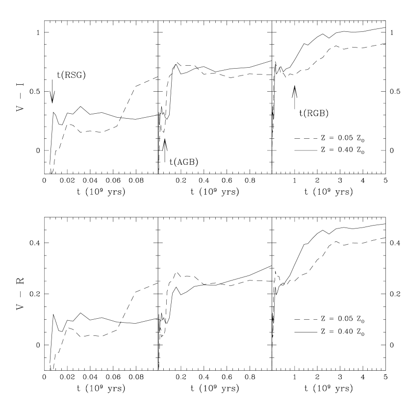
Figure 9: Models of Single Stellar Populations (SSP) from Bressan, Chiosi & Fagotto (1994). Top panels: V–I Cousins colours. Bottom panels: V–R Cousins colours. The three panels for each colours are the same with consecutive blow-up of younger age ranges (0-$5\times 10^{9}$, 0-$1\times 10^{9}$, 0-$1\times 10^{8}$ yrs). Solid lines are models for $Z=\frac{2}{5}Z_{\odot}$. Dashed lines are models for $Z=\frac{1}{20}Z_{\odot}$.

Knowledge of the stellar content is an important prerequisite before one can answer questions regarding the physical processes relevant for understanding star formation and the chemical evolution in HII galaxies. In order to have a handle on the properties of the stellar populations, one can compare the observed properties of the galaxies such as integrated colours, equivalent widths of the spectral lines, total luminosities, etc, with evolutionary population synthesis models which are designed to predict such observables. Slight different predictions of the observables may arise from different evolutionary population models from different treatment and/or input parameters regarding the library of stellar evolutionary tracks used to calculate isochrones in the theoretical colour magnitude diagrams (CMD), library of observed stellar spectra to derive the integral spectral energy distribution which will lead to magnitudes and colours, and the assumptions for star formation and chemical enrichment. Therefore, one needs to choose which model one will adopt to compare with observations depending on available constraints of interest in each case. Very often the results are not unique and only global properties of the observed galaxy are retrieved.

In this section we have compared the results of three recent evolutionary models for an episode of star formation of no duration which synthesize broad band colours of the immediate interest. Firstly, we have chosen two models (Cerviño & Mas Hesse 1994, Leitherer & Heckman 1995) which describe in detail the early evolution of the starburst with a short time resolution ($\Delta\sim 0.1$ Myrs). These models are based on the most up-to-date input physics for the theory of stellar atmospheres, stellar winds, and stellar evolution. Both models also include nebular continuum emission but do not consider gaseous line emission. They are, however, optimized for the treatment of the massive stars in the starburst. As discussed by these authors, massive stars ($M>5~{}M_{\odot}$ in the Zero Age Main Sequence) evolve in only a few million years, therefore it is reasonable to assume that they have all formed coevally in an instantaneous burst of star formation. Other observational properties also put tight constraints on the age and composition of the stellar populations in HII galaxies. The equivalent width of H$\beta$ has been shown to be an age indicator for young bursts of star formation (Copetti, Pastoriza & Dottori 1986). The typically large values for this observable in HII galaxies indicate that the present burst of star formation must be younger than a few 10⁷ years. In addition, in galaxies where the Wolf-Rayet (WR) star signatures are detected, the inferred large ratio of the number of Wolf-Rayet stars to the total number of massive stars that undergo a Wolf-Rayet phase [WR/(WR+O)] provide a strong evidence towards the relatively short duration of these intense star formation processes, since they can not be reproduced assuming a constant star formation rate (Vacca & Conti 1992). For these reasons we only consider Single Stellar Population (SSP) models in our analysis.

For the prediction of the evolution of the stellar system after all ionizing stars have exploded as supernovae we have made use of the detailed chemical-spectro-photometric models of population synthesis by Bressan, Chiosi & Fagotto (1994) who include all evolutionary phases, from the main sequence till late stages of stellar evolution. Bressan, Chiosi & Fagotto models (1994) do not include the nebular continuum emission, which in any case is not significant in the optical regime, nor gaseous line emission. However, since it was designed to represent the evolution of the stellar population of elliptical galaxies it follows the evolution to older ages. This will be useful when we want to search for the underlying older stellar populations by comparing with the colours of the extensions of the sample of HII galaxies.

Table 11 shows some of the basic parameters for the models in question. Figure 8 shows the predictions of the different models for the optical (V–I and V–R) Cousins colours of a starburst for two metallicities ($\sim 1/10$ solar, solar). In all cases the published Johnson colours have been transformed to the observed Cousins photometric system using the formulae given in Bessell (1979). Agreement is reasonably good between Leitherer & Heckman’s models (dashed lines) with Cerviño & Mas Hesse’s (dotted lines) who use the old and the new, respectively, evolutionary tracks from the Geneva group. They are very similar in V–R at both metallicities, but disagree to up to $\sim 0.4$ mag in V–I at low metallicities. Bressan, Chiosi & Fagotto models which are not optimized to describe the evolution of the starburst, although it uses all evolutionary phases according to the Padova tracks, are only in general agreement with the other models. The single largest discrepancy seems to be associated with the lack of a strong supergiant burst in the Padova colours at a few million years, notably at solar metallicity.

In order to  “disentangle ” ages and metallicity of the synthesized stellar population models we have assumed the gas abundances derived from the emission line fluxes to be a reasonable upper limit of the metallicity of the underlying population. Therefore, we are only concerned with the models of low metallicity (Z $\sim$ 1/10 Z_⊙). For this regime, the upper panels for both colours of figure 8 show that these optical colours alone are not very sensitive to the early evolution of the starburst ($t<2\times 10^{7}$ yrs). This trend is followed by any of the three models. One can only say that a low metallicity starburst with colours bluer than V–R $<0.1$ and V–I $<0.3$ will be dominated by a single stellar population younger than a few $10^{7}$ yrs.

Figure 9 shows the colour evolution of a SSP for two different sub-solar compositions (Z = 0.001 as dashed lines and Z = 0.008 as solid lines; in this unit Z_⊙ = 0.02) from Bressan, Chiosi & Fagotto (1994). Upper panels show the predictions of V–I and lower panels the predictions for V–R Cousins colours. The results refer to the Salpeter IMF with $m_{l}=0.85$  $\hbox{M}_{\odot}$ and $m_{u}=120$  $\hbox{M}_{\odot}$. Details of the construction of the models can be found in their paper (Bressan, Chiosi & Fagotto 1994). The panels from the left to the right show different age ranges of the same models in order to illustrate the three main phases which characterize the evolution of a SSP. These may be called  “phase transitions ” which cause the models to predict sudden changes to the colours as the evolution proceeds at the appearance of particular evolutionary phases of different types of star. These  “jumps ” to redder colours are most remarkable at the appearance of the asymptotic giant branch (AGB) at about $10^{8}$ yrs and the red giant branch (RGB) stars at about $10^{9}$ yrs (see Table 1 in Bressan, Chiosi & Fagotto). The AGB and RGB phases can be experienced by stars of different initial masses and lifetimes, hence characteristic ages. These ages are shown as arrows in figure  9.

The small difference in chemical composition of the models shown in figure 9 at the low metallicity regime does not change the predictions of these optical colours by very much. For $Z=1/20Z_{\odot}$ (dashed lines) the colours evolve in a slightly bluer path than at $Z=2/5Z_{\odot}$ (solid lines). The main difference occurs at very early stages of the evolution (at $\sim 10^{7}$ yrs) with the appearance of the first red supergiant phase (RSG) of massive stars. At low metallicities, helium ignition occurs at hot effective temperatures for stars with higher initial masses. These stars start burning helium as blue supergiants (BSG) and become RSG stars only at the end of the helium burning phase (Garcia-Vargas, Bressan & Díaz 1995). For these reasons the model for Z=0.001 (1/20 Z$\odot$), dashed lines in figure 9, do not produce the small peak due to the RSG phase at about $6\times 10^{6}$ yrs as do the models for higher metallicity.

Figure 10: Dereddened colour-colour diagrams. a) Total observed colours. b) Colours of the starburst region alone. In these panels we draw lines joining the uncorrected starburst colours (filled circles) to the corrected colours (crosses) to illustrate the effect on these colours when we subtract the emission line contribution. c) Colours of the extensions. The stellar evolutionary models are shown in the figure. Labels (numbers) are log(age).

5.7 Comparison of HII galaxy colours with evolutionary population models

To set limits on the star formation histories in these star forming dwarfs, we have compared Bressan, Chiosi & Fagotto ’s models with the colours of the present sample of HII galaxies.

Figure 10 a.b.c show the de-reddened colour-colour diagrams for the total colours (integrated colours of the whole galaxy), for the starburst colours and for the colours of the extensions, respectively (see Section 4.5 for a description of how these two components are separated). The colours of the extensions are corrected for galactic extinction only. The colours of the starburst are corrected for total line of sight extinction using the estimate from the Balmer decrement [C(H$\beta$)] derived from the spectrophotometric information in SCHG, assuming case B recombination. The typical estimated internal photometric errors are shown in each panel as a solid line cross. The dashed line error cross in figure 10b corresponds to the estimated error in the emission line subtracted colours of the starburst (starburst continuum colours).

Figure 10a shows the colour-colour diagram for the integrated colours of the whole galaxy corrected for galactic extinction. The dot-dashed lines in this figure show the direction to which the correction for the contribution of emission lines in the broad band filters will shift the total colours. The crosses represent the colours after this correction has been applied. The correction for line emission applied here is described in Appendix A. In this panel the solid line represents the single stellar population (SSP) models at 1/20th of solar metallicity (Z=0.001) from Table 3 of Bressan, Chiosi & Fagotto (1994). The dotted line is the starburst model of Cerviño & Mas-Hesse (1994) and the dashed line is the starburst model of Leitherer & Heckman (1995) as shown. It is clear from this top left panel that there is an inconsistency between the stellar population models and the observed colours of HII galaxies. The inconsistency still remains even after subtraction of the contribution of the emission lines within the starburst region. Therefore, we have separated the starburst from the extensions of each galaxy in order to have a better handle on the colours of the two distinct stellar population components. Thus, we have attempted to put constraints on the age of the stellar population both of the stellar system within the starburst and the underlying stellar system by comparing these derived colours with an adopted evolutionary model. From what follows, we have adopted models with metallicity as near as possible to the upper limit imposed by the observed heavy element abundance derived from the nebula emission. Therefore, the models are all low metallicity (Z = 0.1  $\hbox{Z}_{\odot}$).

5.7.1 The age of the starburst

Figure 10b shows the observed colours of the starburst (filled circles). The dashed lines again, represent the shift of the points in this diagram caused by the subtraction of the flux contribution in the broad band filters by the nebular emission lines ([OIII], H$\beta$ and H$\alpha$). Thus, the tip of the line represents the starburst continuum colours. We have also subtracted the contribution of the underlying galaxy to the colours within the starburst region, assuming a constant surface brightness of the underlying galaxy as given in Table 10.

From this figure one can see that most of the starbursts have colours that fall significantly far from the locus of the colours predicted for very young single stellar bursts ($\approx 10^{7}$ yrs), considering the constraints on the age and duration of the burst by the spectroscopic observations (Coppetti, Pastoriza & Dottori 1986; Vacca & Conti 1992; Cerviño & Mas-Hesse 1994; Garcia-Vargas, Bressan & Díaz 1995). Shown in this figure as filled squares is the model by Leitherer & Heckman (1995) from 10⁶ to 10⁸ yrs and as filled triangles the models by Cerviño & Mas-Hesse (1994) from 10⁶ to 10⁷ yrs. As can be seen from table 9, the starburst colours of IIZw40 fall outside the range plotted here. This is a very low galactic latitude object and the extinction correction is relatively more uncertain.

At this point we are unable to derive definitive conclusions from the broadband optical colours alone about the stellar content in the starburst in HII galaxies. Various sources of uncertainties may be the causes of the discrepancies. Some of them are:

• Reddening: We may be strongly underestimating the reddening of the stellar population within the starburst by using the estimate from the emission line ratio and assuming case B recombination.

• Underlying galaxy: The assumption of a  “sheet-like ” underlying galaxy of constant surface brightness may be a poor one. We may be underestimating the contribution of a underlying population of stars formed previous to the present burst.

• The emission line correction: An assumption of a constant surface brightness distribution of the emission lines is rather crude. A better account for the emission line contribution and its surface brightness distribution can be achieved in an analogous way to the procedure here with accurate narrow band surface photometry centered on either H$\alpha$ or [OIII] lines.

• Models: The late stages of massive star evolution may not be well prescribed by the models, mainly at low metallicities. The uncertainties include the photoionization and energy output from massive stars, the relative numbers of red and blue supergiants, the evolution of Wolf-Rayet stars and the rate of Type II supernovae, as emphasized by recent comparative studies of evolutionary synthesis models by Charlot, Worthey & Bressan (1996) and García-Vargas, Bressan & Leitherer (1996).

The role of many parameters in stellar evolutionary population synthesis models are still worthy of close scrutiny and detailed study. But from the observational point of view, we believe there are still methodologies (like the one presented here) of data analysis that can be improved and devised in order to probe the stars in starburst.

5.7.2 The age of the underlying galaxy

Figure 10c shows the colour-colour diagram for the extensions of HII galaxies. These regions are beyond the ionized region and represent the underlying population formed in previous episodes of star formation. The position of the galaxy colours in this diagram seems to suggest that the underlying galaxy in HII galaxies have ages ranging from a few 10⁹ to 10¹⁰ years when compared with the SSP models with standard IMF at low metallicity of Bressan, Chiosi & Fagotto (1994). These are indications, therefore, of an intermediate age population ($\sim 10^{9}$ yrs) in HII galaxies.

This brief stellar population analysis is consistent with the findings of the comparison with the colours of other dwarf galaxies and seems to rule out the young galaxy hypothesis for these systems. They are unlikely to be experiencing their very first burst of star formation.

5.7.3 A composite model for the underlying galaxy

Figure 11: Composite models. Extension colours

We have investigated the properties of the underlying galaxy deduced from the colours beyond the region which is presently undergoing violent star formation (the extensions) in order to infer what one expects to observe in the quiescent periods of HII galaxies. Figure 11 shows two SSP composite models, as a function of the fraction of the total mass involved in the burst (the strength of the burst), one representing a burst of $10^{7}$ yrs old (long dashes) superposed on a $10^{10}$ yr old underlying galaxy, the other a burst of $1.2\times 10^{8}$ yrs old (short dashes) superposed on a $10^{10}$ yr old underlying galaxy. A recent episode of star formation ($10^{7}$ yrs old) superposed on an old galaxy would make the colours of the underlying galaxy much bluer than observed even if only a small fraction of the total mass participated in this event (long dashes). On the other hand, if no other burst occured since the very first episode $10^{10}$ yrs ago the colours would have remained redder than observed. The fact that the observed colour of the extensions lie roughly between the locus of the evolution of a composite system with a $1.2\times 10^{8}$ yr old event and a pure old galaxy (short dashes) suggests that HII galaxies may have undergone an intermediate episode of star formation approximately $10^{9}$ yrs ago and the light now is dominated by the intermediate mass stars in the AGB phase. Although we do not claim that these results are conclusive, they seem to be compatible with the view of episodic star formation followed by long quiescent periods for HII galaxies.

Separating the burst and extension has improved the compatibility with the models for the extension. However, the models remained inconsistent with the observed colours of the burst. The method applied here, however, may be further improved and useful specially with deeper observations and a wider spectral dynamical range. Ferguson (1994) has also compared the B-V and V–I colours of a sample of different types of dwarf galaxies from the literature with the same evolutionary models used here (Bressan, Chiosi & Fagotto 1994) as well as with models of Worthey (1994). He has shown that the observed colours are incompatible with the expectations from these stellar population models. Therefore, until further tests of the calibration of the galaxy colours and the uncertainties and application of the models are better understood, we will simply take these results as tentative. These results show that if models do not fit the observations of present day  “young ” systems, there seems to be little hope for studies of young systems at high $z$ where additional uncertainties are present (e.g. K corrections, lack of spatial resolution or spectrophotometric information).

6 Conclusions

We have presented evidence from a morphological, photometric and structural point of view that HII galaxies show a wide range of morphologies with their own characteristics, despite of sharing the common property of having a dominant giant HII region. The very cause of the enhanced star formation or possible mechanisms which may have triggered the starburst may have been different in different types of objects. While in more compact single systems the internal dynamics, stochastic star formation or propagating star formation may have a major role, for more luminous systems mergers may have had their act in play.

Some of the main conclusions are:

• We have confirmed the adequacy of the broad classification scheme, devised in Telles, Melnick & Terlevich (1996), namely that, HII galaxies may be described as two different classes of objects:

  • Type I HII galaxies ($M_{\rm V}<-18.5$) are luminous, have larger emission line widths and have marginally higher heavy metal abundances, and show signs of being interacting or merging systems. The most luminous Type I’s also have small equivalent widths of W(H$\beta$).

  • Type II HII galaxies ($M_{\rm V}>-18.5$) are compact and regular. They tend to be marginally more metal deficient and show no signs of being products of interactions or mergers.

• The optical colours of the underlying galaxies are similar to the colours of late type low surface brightness galaxies. These may be good candidates for being the quiescent counterparts of HII galaxies.

• Evolutionary models agree only qualitatively among themselves. They, however, fail to fit quantitatively the observed colours of the starburst in low metallicity HII galaxies to a few tenths of magnitude. We fear that the predictions of the models for the evolution of young galaxies at high redshift may result in even larger uncertainties.

• The comparison of the observed colours with models of evolutionary population synthesis models are inconclusive. This is a consequence of uncertainties both in the observed colours and perhaps more seriously, in the models themselves. In any case, if the models are right for old stellar systems at low metallicity, the colours of the underlying galaxy in HII galaxies are not compatible with them being truly young galaxies having their first burst of star formation. They have indicated the possible presence of an intermediate age population of approximately 1 Gyr ago, suggestive of an episodic mode of star formation for HII galaxies. Surface photometry in the near-infrared, together with the results presented here, may help put more strict constraints on the star formation history in HII galaxies.

Appendix A Correction for emission-line contamination

The approach used here for the correction for the contamination by emission lines of the broad band CCD images follows closely the one used by Salzer, MacAlpine & Boroson (1989) with only a difference on the size factor and the fact that here we deal with the V, R and I bandpass and exclude B as described below.

The colours of a galaxy with strong gaseous emission may be significantly different from the continuum-only colour. For objects with small redshift, H$\beta$ and [OIII]$\lambda\lambda$4959,5007 will be redshifted into the V bandpass and H$\alpha$ will fall well into the R bandpass. The I bandpass, however, is virtually unaffected due to the absence of comparatively strong gaseous emission and also due to its broader filter width.

The contribution of the emission lines to the total flux is then corrected in the following manner:

$${\cal I}_{Total}(\lambda,r)={\cal I}_{gas}(\lambda,r)+{\cal I}_{continuum}(\lambda,r)$$

where ${\cal I}$ is the intensity at a given wavelength and distance from the center. Hence,

$${\cal F}_{Total}^{i}(r)=\int_{i}{\cal I}_{Total}(\lambda,r)\times T_{i}(\lambda)d\lambda$$

$$=\int_{i}{\cal I}_{g}(\lambda,r)\times T_{i}(\lambda)d\lambda+\int_{i}{\cal I}_{c}(\lambda,r)\times T_{i}(\lambda)d\lambda$$

$${\cal F}_{Total}^{i}(r)={\cal F}_{g}^{i}(r)+{\cal F}_{c}^{i}(r)$$

where ${\cal F}_{Total}^{i}(r)$ is the total flux in filter $i$ and $T_{i}(\lambda)$ is the combined normalized CCD sensitivity and filter transmittance at a wavelength $\lambda$.

For the contribution of an emission line $l$, we can describe the intensity by

$${\cal I}_{g}(\lambda,r)={\cal F}_{g}^{i}(r)\times\delta(\lambda-\lambda_{l})={\cal I}_{c}(\lambda,r)\times W_{l}(r)\times\delta(\lambda-\lambda_{l})$$

$W_{l}(r)$ is the equivalent width of line $l$. Hence,

$${\cal F}_{g}^{i}(r)=\int_{i}{\cal I}_{c}(\lambda,r)\times W_{l}(r)\times\delta(\lambda-\lambda_{l})\times T_{i}(\lambda)d\lambda$$

$$={\cal I}_{c}(\lambda_{l},r)\times W_{l}(r)\times T_{i}(\lambda_{l})$$

and now $T_{i}(\lambda_{l})$ is the value for the combined normalized CCD sensitivity and filter transmittance at redshifted wavelength of the emission line $l$.

Assuming a plane continuum [${\cal I}_{c}(\lambda,r)={\cal I}_{c}(r)$] one would have for its contribution to the total flux the following:

$${\cal F}_{c}^{i}(r)={\cal I}_{c}(r)\times\Delta\lambda_{i}$$

where $\Delta\lambda_{i}=\int_{i}T_{i}(\lambda)d\lambda$ is the filter bandpass width. Finally,

$${\cal F}_{Total}^{i}(r)={\cal I}_{c}(r)\times W_{l}(r)\times T_{i}(\lambda_{l})+{\cal I}_{c}(r)\times\Delta\lambda_{i}$$

$$={\cal F}_{c}^{i}(r)\times{\sum[\frac{W_{l}(r)}{\Delta\lambda_{i}}\times T_{i}(\lambda_{i})]+1}$$

where the $\sum$ indicates that one such term for each line $l$ considered in filter $i$ should be included.

Salzer, MacAlpine & Boroson (1989) introduce a multiplicative factor ${\cal R}$ in the sum which is the ratio of the area of the slit to the area where their broad and measurements were made,

$${\cal F}_{c}^{i}=\frac{{\cal F}_{Total}^{i}}{[\sum\frac{W_{l}}{\Delta\lambda_{i}}\times T_{i}(\lambda_{i})\times{\cal R}]+1}$$

As opposed to Salzer, MacAlpine & Boroson (1989) though we are only correcting the flux within the burst region of a galaxy, not the total galaxy flux, which has been separated by subtracting the narrow band CCD image from the broad band ones to discriminate the region of gaseous emission, thus for us $\cal R=$ 1. This does not solve the problem of the spatial variation of surface brightness including the variation of the strength of the lines W(H$\beta$) across the burst region. It is worth noting as well that the correction for the V–R colours, just as the B-V colours of Salzer, MacAlpine & Boroson are small because they are differential between both fluxes. However, the correction in V–I and R–I colours will be much larger since there is no correction in the I fluxes. Correction for the total colours of the galaxy will be larger the larger the contribution of the burst region to the total fluxes, or similarly the larger the ratio of burst area to total area.

References

- [Bachall 1977] Bessell M.S., 1979, Publ. astr. Soc. Pacif. , 91, 589
- [Bachall 1977] Binggeli B., 1985, in “Star Forming Dwarf Galaxies ”, eds. D.Kunth, T.X.Thuan and J.Tran Thanh Van, èditions Frontières Gif Sur Yvette, France, p. 53
- [Bachall 1977] Bothun G.D., Impey C.D. & Malin D.F., 1991, ApJ, 376, 404
- [Bachall 1977] Bothun G.D., Mould J.R., Wirth, A. & Caldwell N., 1985, AJ, 91, 697
- [Bachall 1977] Bothun G.D., Mould J.R., Caldwell N. & Macgillivray H.T., 1986, AJ, 92, 1007
- [Bachall 1977] Bressan A., Chiosi C. & Fagotto F., 1994, ApJ, 94, 63
- [Bachall 1977] Burstein D. & Heiles C., 1982, AJ, 87, 1165
- [Bachall 1977] Cerviño M. & Mas-Hesse J.M., 1994, A&A, 284, 749
- [Bachall 1977] Charlot S., Worthey G., Bressan A., 1996, ApJ, 457, 625
- [Bachall 1977] Conti P.S., Vacca W.D., 1994, ApJL, 423, L97
- [Bachall 1977] Coppetti M.V.F., Pastoriza M.G. & Dottori H.A., 1986, A&A, 156, 111
- [Bachall 1977] Davies J.I. & Phillipps S., 1988, MNRAS, 233, 553
- [Bachall 1977] Elmegreen B., 1992, in “Star Formation in Stellar systems ”, eds. G.Tenorio-Tagle, M.Prieto & F.Sánchez, Cambridge Univ. Press, Cambridge, p. 381
- [Bachall 1977] Faber S.M. & Lin D.N.C., 1983, ApJ, 266, 17
- [Bachall 1977] Ferguson.H.C., 1994, in “ESO/OHP Workshop on Dwarf Galaxies ”, eds. G.Meylan and P.Prugniel, ESO, Garching bei München, p. 475
- [Bachall 1977] Gallagher J.S. & Hunter D.A., 1987, AJ, 94, 43
- [Bachall 1977] Garcia-Vargas M.L., Bressan A. & Díaz A.I., 1995, A&AS, 112, 13
- [Bachall 1977] García-Vargas M.L., Bressan A., Leitherer C., 1996, in preparation
- [Bachall 1977] García-Vargas M.L., González-Delgado R.M., Perez E., Alloin, D., Díaz A.I. & Terlevich, E. 1996, ApJ submitted
- [Bachall 1977] Gerola H., Seiden P.E. & Schulman L.S., 1980, ApJ, 242, 517
- [Bachall 1977] González-Delgado R., Pérez E., Díaz A., García-Vargas M.L., Terlevich E., Vilchez J.M., 1995, ApJ, 439, 604
- [Bachall 1977] Guzmán,R., Koo,D.C., Faber,S.M., et al. , 1996, ApJL, 460, L5
- [Bachall 1977] Huchra J., 1977, ApJ, 217, 928
- [Bachall 1977] Impey C., Bothun G. & Malin D., 1988, ApJ, 330, 634
- [Bachall 1977] Koo, D.C., 1994, in IAU Symp. 168, “Examining the Big Bang and Diffuse Background Radiation, ed. M. Kafatos (Dordrecht:Kluwer)
- [Bachall 1977] Koo,D.C., Guzmán,R., Faber,S.M., Illingworth,G.D. & Bershady,M.A., 1995, ApJL, 440, L52
- [Bachall 1977] Landolt A.U., 1983, AJ, 88, 439
- [Bachall 1977] Leitherer C. & Heckman T.M., 1995, ApJs, 96, 9
- [Bachall 1977] Loose H.H. & Thuan T.X., 1985, in “Star Forming Dwarf Galaxies ”, eds. D.Kunth, T.X.Thuan and J.Tran Thanh Van, editions Frontières Gif Sur Yvette, France, p. 73
- [Bachall 1977] Mazzarella J.M. & Boroson T.A., 1993, ApJs, 85, 27
- [Bachall 1977] McGaugh S.S., 1991, ApJ, 380, 140
- [Bachall 1977] McGaugh S.S. & Bothun G.D., 1994, AJ, 107, 530
- [Bachall 1977] Melnick J., Terlevich R. & Moles M., 1988, MNRAS, 235, 297
- [Bachall 1977] Moles M., Garcia-Pelayo J.M., del Río G. & Lahulla F., 1987, A&A, 186, 77
- [Bachall 1977] NOTNEWS, Nordic Optical Telescope Newsletter, Dec 1989, 8
- [Bachall 1977] Pagel B.E.J., Edmunds M.G., Blackwell D.E., Chun M.S. & Smith G., 1979, MNRAS, 189, 95
- [Bachall 1977] Pagel B.E.J., Simonson E.A., Terlevich R. & Edmunds M.G., 1992, MNRAS, 255, 325
- [Bachall 1977] Rönnback J. & Bergvall N., 1994, A&AS, 108, 193
- [Bachall 1977] Salzer J.J., 1989, ApJ, 347, 152
- [Bachall 1977] Salzer J.J., MacAlpine G.M. & Boroson T.A., 1989, ApJs, 70, 447
- [Bachall 1977] Sargent W.L.W., 1970, ApJ, 160, 405
- [Bachall 1977] Sargent W.L.W. & Searle L., 1970, ApJL, 162, L155
- [Bachall 1977] Schombert J.M., Bothun G.D., Schneider S.E. & McGaugh S.S., 1992, AJ, 103, 1107
- [Bachall 1977] Telles E., 1995, Ph.D. thesis, University of Cambridge
- [Bachall 1977] Telles E. & Terlevich R., 1993, Astrophys. Space Sci., 205, 49 (TT93)
- [Telles & Terlevich 1995] Telles E. & Terlevich R., 1995, MNRAS, 275, 1
- [Bachall 1977] Telles E., Melnick J., Terlevich R., 1996, MNRAS, submitted
- [Terlevich et al. 1991] Terlevich R., Melnick J., Masegosa J., Moles M. & Copetti M.V.F., 1991, A&AS, 91, 285 (SCHG)
- [Bachall 1977] Vacca W.D., 1994, in ”Violent Star Formation: From 30 Doradus to QSO’s ”, ed. G. Tenorio-Tagle, Cambridge Univ. Press, Cambridge, p. 297
- [Bachall 1977] Vacca W.D. & Conti P.S., 1992, ApJ, 401, 543
- [Bachall 1977] Varela A., 1992, Ph.D. thesis, Instituto de Astrofisica de Canarias
- [Bachall 1977] Wade R.A., Hoessel J.G., Elias J.H. & Huchra J.P., 1979, Publ. astr. Soc. Pacif. , 91, 35
- [Bachall 1977] Walborn N.R., 1991, in “Massive Stars in Starbursts ”, eds. C. Leitherer, N.R. Walborn, T.M. Heckman & C.A. Norman, Cambridge Univ. Press, Cambridge, p. 145
- [Bachall 1977] Weedman D.W., Feldman F.R., Balzano V.A., Ramsey L.W., Sramek R.A., Wu C.-C., 1981, ApJ, 248, 105
- [Bachall 1977] Worthey G., 1994, ApJs, 95, 107
- [Bachall 1977] Zaritsky D. & Lorrimer S.J., 1993, in “The Evolution of Galaxies and Their Environment ”, eds. D.Hollenbach, H.Thronson & J.M.Shull, NASA Conference Publication 3190, p. 82
- [Bachall 1977] Zwicky F., 1964, ApJ, 140, 1467