Constraints on $h$, $\Omega_{b}$ and $\lambda_{o}$ from Cosmic Microwave Background Observations

Abstract

In this paper we compare data to theory. We use a compilation of the most recent cosmic microwave background (CMB) measurements to constrain Hubble’s constant $h$, the baryon fraction $\Omega_{b}$, and the cosmological constant $\lambda_{o}$. We fit $h$-, $\Omega_{b}$- and $\lambda_{o}$-dependent power spectra to the data. The models we consider are flat cold dark matter (CDM) dominated universes with flat ($n_{s}=1$) power spectra, thus the results obtained apply only to these models. CMB observations can exclude more than half of the $h-\Omega_{b}$ parameter space explored. The CMB data favor low values of Hubble’s constant; $h\approx 0.35$. Low values of $\Omega_{b}$ are preferred ($\Omega_{b}\sim 0.03$) but the $\chi^{2}\>$minimum is shallow and we obtain $\Omega_{b}<0.28$. A model with $h\approx 0.40$, $\Omega_{b}\approx 0.15$ and $\Omega_{cdm}\approx 0.85$ is permitted by constraints from the CMB data, BBN, cluster baryon fractions and the shape parameter $\Gamma$ derived from the mass density power spectra of galaxies and clusters.

For flat-$\lambda_{o}$ models, the CMB data, combined with BBN constraints exclude most of the $h-\lambda_{o}$ plane. Models with $\Omega_{o}\approx 0.3$, $\lambda_{o}\approx 0.7$ with $h\approx 0.75$ are fully consistent with the CMB data but are excluded by the strict new $q_{o}$ limits from supernovae (Perlmutter et al.1997). A combination of CMB data goodness-of-fit statistics, BBN and supernovae constraints in the $h-\lambda_{o}$ plane, limits Hubble’s constant to the interval $0.23<h<0.72$.

Key words: cosmic microwave background — cosmology: observations

1 Introduction

A new technique is coming on-line producing a small revolution in our ability to evaluate cosmological models (Bond et al.1994). Measurements of fluctuations in the cosmic microwave background (CMB) over a large range of angular scales have become sensitive enough to distinguish one model from another. This technique is truly cosmological and independent of previous methods. It probes scales much larger and times much earlier ($z\approx 1000$) than more traditional techniques which rely on supernovae, galaxies, quasars and other low-redshift objects.

Our ignorance of $h$, $\Omega_{b}$ and $\lambda_{o}$ is large and there are many inconsistent observational results. For example, after 60 years of effort the favorite Hubble constants of respected cosmologists can differ by more than a factor of 2 ($0.40\mathrel{\mathchoice{\vbox{\offinterlineskip\halign{\hfil$\displaystyle#$\hfil\cr<\cr\sim\cr}}}{\vbox{\offinterlineskip\halign{\hfil$\textstyle#$\hfil\cr<\cr\sim\cr}}}{\vbox{\offinterlineskip\halign{\hfil$\scriptstyle#$\hfil\cr<\cr\sim\cr}}}{\vbox{\offinterlineskip\halign{\hfil$\scriptscriptstyle#$\hfil\cr<\cr\sim\cr}}}}h\mathrel{\mathchoice{\vbox{\offinterlineskip\halign{\hfil$\displaystyle#$\hfil\cr<\cr\sim\cr}}}{\vbox{\offinterlineskip\halign{\hfil$\textstyle#$\hfil\cr<\cr\sim\cr}}}{\vbox{\offinterlineskip\halign{\hfil$\scriptstyle#$\hfil\cr<\cr\sim\cr}}}{\vbox{\offinterlineskip\halign{\hfil$\scriptscriptstyle#$\hfil\cr<\cr\sim\cr}}}}0.90$) with error bars small compared to this interval. Thus, information on Hubble’s constant and other cosmological parameters from the independent and very high redshift CMB data is important. Over the next decade observations at small angular scales have the potential to determine many important cosmological parameters to the $\sim 1\%$ level (Jungman et al.1996). We expect CMB measurements to tell us the ultimate fate of the Universe ($\Omega_{o}$), what the Universe is made of ($\Omega_{b}$, $\Omega_{cdm}$) and the age and size of the Universe ($h$) with unprecedented precision.

The COBE detection of temperature fluctuations in the CMB (Smoot et al.1992, Bennett et al.1996) has constrained the amplitude and slope of the power spectrum at large angular scales. Scott et al.(1995), using a synthesis of the most current CMB measurements at that time, demonstated the existence of the predicted acoustic peak. Using compilations of CMB measurements, Ratra et al.(1995), Ganga et al.(1996), Górski et al.(1996), White et al.(1996) have compared groups of favored models to the data and obtained interesting constraints on $\Omega_{o}$, $n$ and the normalizations of various flat and open CDM models.

The most recent ground-based and balloon-borne experiments (Netterfield et al.1997, Scott et al.1996, Platt et al.1996, Tanaka et al.1996) are providing increasingly accurate CMB fluctuation measurements on small angular scales. In this work we take advantage of these new measurements and of a fast Boltzmann code (Seljak & Zaldarriaga 1996) to make a detailed exploration of two large regions of parameter space: the $h-\Omega_{b}$ and $h-\lambda_{o}$ planes. Such an approach allows us to place independent CMB-derived constraints on $h$, $\Omega_{b}$ and $\lambda_{o}$ based on goodness-of-fit statistics.

Our results are valid only in the context of the models we have considered; we assume COBE normalized, Gaussian, adiabatic initial conditions in spatially flat universes ($k=0$, $\Omega_{o}+\lambda_{o}=1$) with Harrison-Zel’dovich ($n_{s}=1$) temperature fluctuations. For Gaussian fluctuations the power spectra, $C_{\ell}$, uniquely specify the models. Our limits include estimates of the uncertainty due to the COBE normalization uncertainty as well as the Saskatoon absolute calibration uncertainty. We use $h=H_{o}/100$ km s^-1 Mpc^-1.

Our CMB-derived constraints on $h$, $\Omega_{b}$ and $\lambda_{o}$ are independent of BBN and other cosmological tests. Where the CMB constraints are not as tight as other methods, the existence of overlapping regions of allowed parameter space is an important consistency check for both; unknown systematic errors can be uncovered by such a comparison.

In Section 2 we describe the $\chi^{2}\>$calculation. In Section 3 we provide an overview of the physics of fluctuations and the power spectrum models used in the fit. In Sections 4 and 5 we discuss our results for the $h-\Omega_{b}$ and $h-\lambda_{o}$ planes respectively and combine them with a variety of other cosmological constraints. In Section 6 we summarize and discuss our results.

2 Data Analysis

2.1 The Recipe

$\bullet$ assemble all available CMB experimental results with the corresponding window functions

$\bullet$ determine the region of parameter space one would like to explore (we choose the $h-\Omega_{b}$ and $h$ - $\lambda_{o}$ planes for spatially flat models)

$\bullet$ use a fast Boltzmann code (Seljak & Zaldarriaga 1996) to obtain the power spectra for a matrix of models covering the desired region of parameter space

$\bullet$ convolve each model with the experimental window functions and fit the result to the data by producing a $\chi^{2}\>$surface over the chosen parameter space

$\bullet$ compare the results with other cosmological constraints

2.2 The Equations

We calculate the $\chi^{2}\>$surface over a matrix of models

$$\chi^{2}(i,j)=\sum_{N=1}^{N_{exp}}\left[\frac{\delta T_{\ell_{eff}}^{data}(N)-\delta T_{\ell_{eff}}^{model}(N,i,j)}{\sigma^{data}(N)}\right]^{2},$$ (1)

and use it to indicate the regions of parameter space preferred by the data. The sum is over the CMB detections plotted in Figure 1 and listed in Table 1 in the form of flat band power: $\delta T_{\ell_{eff}}^{data}(N)$ with the corresponding errors $\sigma^{data}(N)$. The models are indexed in the 2-D parameter space by $i$ and $j$. The band power estimates of the data and models are defined respectively as

$$\delta T_{\ell_{eff}}^{data}(N)\>\> = \>\>\frac{\delta T^{obs}_{rms}(N)}{\sqrt{I(W_{\ell}(N))}}$$ (2)

$$= \left[\frac{1}{I(W_{\ell}(N))}\sum_{\ell=2}^{\ell_{max}}\frac{(2\ell+1)}{4\pi}C_{\ell}(real)W_{\ell}(N)\right]^{1/2}$$

$$\delta T_{\ell_{eff}}^{model}(N,i,j) = \frac{\delta T^{model}_{rms}(N,i,j)}{\sqrt{I(W_{\ell}(N))}}$$ (3)

$$= \left[\frac{1}{I(W_{\ell}(N))}\sum_{\ell=2}^{\ell_{max}}\frac{(2\ell+1)}{4\pi}C_{\ell}(i,j)W_{\ell}(N)\right]^{1/2},$$

where $\delta T^{obs}_{rms}(N)$ is the rms temperature fluctuation observed by the $Nth$ experiment, $W_{\ell}(N)$ are the experiment-specific window functions (White & Srednicki 1995) and the deconvolving factors $I(W_{\ell}(N))$ are the logarithmic integrals of the $W_{\ell}$ (Bond 1995) defined as

$$I(W_{\ell})=2\pi\sum_{\ell=2}^{\ell_{max}}\frac{(2\ell+1)}{4\pi}\frac{W_{\ell}}{\ell(\ell+1)},$$ (4)

where $\ell_{max}=1200$ since for all $N$, $W_{\ell}(N)\approx 0$ for $\ell>1200$. The angular scale probed by the $N$th experiment is

$$\ell_{eff}(N)=\frac{I(\ell\>W_{\ell}(N))}{I(W_{\ell}(N))}.$$ (5)

In equation (2), the convolution of the unknown real power spectrum of the CMB sky, $C_{\ell}(real)$, with $W_{\ell}$ is the observed temperature rms, $\delta T^{obs}_{rms}$. One cannot compare the rms results from different experiments with each other unless the influence of the window function has been removed, i.e., deconvolved. The division by $I(W_{\ell})$ is this deconvolution and works optimally when $\ell(\ell+1)C_{\ell}(real)$ is a constant across the range of $\ell$ sampled by the experiment. Equation (4) has been written suggestively to clarify this deconvolution. Notice that the models are treated like the real sky: first they are convolved with the window function and then the division by $I(W_{\ell})$ deconvolves the window function. Thus our model points are “convolved-deconvolved” power spectra. Setting $C_{\ell}=a/\ell(\ell+1)$ in equation (2) or (3) yields $\delta T_{\ell_{eff}}=(a/2\pi)^{1/2}=[\ell(\ell+1)C_{\ell}/2\pi]^{1/2}$ which is the origin of the units of the y-axis of Figure 1 and why it is reasonable to plot the input model and the flat band power estimates on the same plot.

Fig. 1.: The power spectrum of observed CMB temperature fluctuations (from Table 1) as a function of angular scale. The FWHM of the window functions are indicated by the horizontal lines at each data point. Two representative models are also plotted; both have $\Omega_{b}=0.05$. The differences between the convolved $h=0.3$ model (large circles) and the measurements is used to calculate a single point of the $\chi^{2}\>$surface shown in Figure 8. The small boxes above and below the Saskatoon points indicate the $\pm 14\%$ absolute calibration uncertainty shared by these 5 points. The dotted line is a 5th order polynomial fit to the data. On the upper axis, $\theta_{FWHM}=(32\>ln\>2)^{1/2}sin^{-1}(\frac{1}{2\ell+1})$ (Bond 1995).

Using the data and equation (3) in equation (1) yields a $\chi^{2}\>$value for every point in the matrix of models. Figure 1 is a picture of the ingredients of our $\chi^{2}\>$calculation. The CMB measurements from Table 1 are plotted. The thick solid line is an $h=0.30$ model with $\Omega_{b}=0.05$. The large open circles are the convolution of this $h=0.30$ model with the experimental window functions. The difference between the resulting “convolved-deconvolved” points and the measurements is used to calculate the $\chi^{2}\>$values. By comparing the data with these “convolved-deconvolved” points rather than with the direct $[\ell(\ell+1)C_{\ell}/2\pi]^{1/2}$ values of the original $h=0.30$ model, we are accounting for the experimental window function even in the regions of sharp peaks and valleys. The discrepancy between the open circles and the original $h=0.30$ model (solid line) is a measure of the necessity of this convolution-deconvolution procedure; it is unnecessary except in the sharp peaks and valleys. The dotted line is a fifth order polynomial fit to the data points and is used in Figures 2 and 5 to represent the data. Notice that the amplitude of the primary acoustic peak in the data is $A_{peak}\sim 80\>\mu$K.

5579F2

Fig. 2.: Representative power spectra showing the $h$- and $\Omega_{b}$-dependence. In each panel $h$ is fixed while $\Omega_{b}$ takes on the values indicated. The largest values of $\Omega_{b}$ have the largest Doppler peaks. Notice that as $h$ increases, $A_{peak}$ increases for large $\Omega_{b}$ but decreases for small $\Omega_{b}$; thus at high $h$ the peak height is an excellent baryometer. The dotted line is the polynomial fit to the data in Figure 1 and is the same in all panels. All models are spatially flat ($k=0$, $\lambda_{o}=0$), Harrison Zel’dovich ($n_{s}=1$) normalized to the COBE 4-year results at $\ell=6$.

Most experimental results contain slightly asymmetric error bars and, most commonly, the upper error bar is larger. For a given data point, this asymmetry constrains models lower than the data point a bit more rigidly than it does models which are higher than the data point. To approximate this asymmetry for the $\chi^{2}\>$calculation, we toggle the error bar depending on whether the model is above or below the data point.

3 CMB Power Spectra

3.1 General Features

Figures 2 and 5 are samples from the matrices of power spectra covering the parameter space explored. They show the influence of $h$, $\Omega_{b}$ and $\lambda_{o}$ on the angular power spectrum of CMB fluctuations. Generic features are:

$\bullet$ a flat Sachs-Wolfe plateau for $\ell\mathrel{\mathchoice{\vbox{\offinterlineskip\halign{\hfil$\displaystyle#$\hfil\cr<\cr\sim\cr}}}{\vbox{\offinterlineskip\halign{\hfil$\textstyle#$\hfil\cr<\cr\sim\cr}}}{\vbox{\offinterlineskip\halign{\hfil$\scriptstyle#$\hfil\cr<\cr\sim\cr}}}{\vbox{\offinterlineskip\halign{\hfil$\scriptscriptstyle#$\hfil\cr<\cr\sim\cr}}}}30$ due to the gravitational potentials of superhorizon-sized density fluctuations.

$\bullet$ a primary acoustic peak at $\ell_{peak}\sim 250$ accompanied by secondary peaks and valleys for $\ell\mathrel{\mathchoice{\vbox{\offinterlineskip\halign{\hfil$\displaystyle#$\hfil\cr>\cr\sim\cr}}}{\vbox{\offinterlineskip\halign{\hfil$\textstyle#$\hfil\cr>\cr\sim\cr}}}{\vbox{\offinterlineskip\halign{\hfil$\scriptstyle#$\hfil\cr>\cr\sim\cr}}}{\vbox{\offinterlineskip\halign{\hfil$\scriptscriptstyle#$\hfil\cr>\cr\sim\cr}}}}2\>\ell_{peak}$

$\bullet$ a cut-off at $\ell\mathrel{\mathchoice{\vbox{\offinterlineskip\halign{\hfil$\displaystyle#$\hfil\cr>\cr\sim\cr}}}{\vbox{\offinterlineskip\halign{\hfil$\textstyle#$\hfil\cr>\cr\sim\cr}}}{\vbox{\offinterlineskip\halign{\hfil$\scriptstyle#$\hfil\cr>\cr\sim\cr}}}{\vbox{\offinterlineskip\halign{\hfil$\scriptscriptstyle#$\hfil\cr>\cr\sim\cr}}}}1000$ due to averaging along the line of sight as the photons traverse the finite thickness of the surface of last scattering

The physics of the primary acoustic peak is the most relevant for our purposes since this peak dominates the fits. At sub-degree angular scales acoustic oscillations of the baryon–photon fluid at recombination produce peaks and valleys in the CMB power spectrum. We may understand their general features by employing the driven oscillator interpretation of Hu (1995) and Hu & Sugiyama (1995a). The waves are set up by the pressure of the photons, which are tightly coupled to the baryons and subject to the driving force of the gravitational potential. Ignoring the neutrinos, there are three particle species present at recombination (baryons, photons and dark matter) which determine two fundamental ratios: the baryon–to–photon ratio, varying as $\Omega_{b}h^{2}$, and the dark matter–to–photon ratio, varying as $\Omega_{cdm}h^{2}$. We expect the physics at this epoch to be largely invariant to changes which leave these quantities unaltered, i.e., we expect $\Omega_{b}h^{2}$ and $\Omega_{cdm}h^{2}$ to control the shape of these oscillations and in particular the height and location of the primary peak $A_{peak}$, $\ell_{peak}$.

Fig. 3.: Contours of $A_{peak}\>[\mu$K]. Although no data were used to make this plot, the $80\>\mu$K contour is thick to indicate the approximate peak height of the data. For large $h$, the strong $\Omega_{b}$-dependence of the peak heights is responsible for the narrow spacing between contours and for the narrow range of $\Omega_{b}$ permitted by the data (see Figure 8). As $h$ decreases, $A_{peak}$ loses its $\Omega_{b}$-dependence thus permitting a wider range of $\Omega_{b}$. The grey band is the region favored by big bang nucleosynthesis: $0.010<\Omega_{b}h^{2}<0.026$ (e.g. Copi et al.1995, Tytler & Burles 1997). All models in this plot have $\Omega_{o}=\Omega_{b}+\Omega_{cdm}=1$ and $\lambda_{o}=0$.

Fig. 4.: Contours of $\ell_{peak}$ for the same models as in Figure 3. The thick 280 contour is indicative of the $\ell_{peak}$ favored by the data. In the lower right, $\ell_{peak}$ is too small to suit the data.

3.2 Effects of $\Omega_{b}h^{2}$ and $\Omega_{cdm}h^{2}$

3.2.1 Peak Height

Figures 2, 3, 4 are a triptych; they show three different ways of looking at the $h-\Omega_{b}$ models we have explored. Figure 2 shows the entire power spectra but only for a sparse sample of parameter space. Each panel shows 5 samples from a vertical strip of Figures 3 and 4. Figures 3 and 4 fully sample the matrix of models but with only one-parameter characterizations of the spectra.

It is important to distinguish aspects of the $\chi^{2}\>$surface produced by the underlying models from the aspects produced by the data. The data currently available are in the range $2\mathrel{\mathchoice{\vbox{\offinterlineskip\halign{\hfil$\displaystyle#$\hfil\cr<\cr\sim\cr}}}{\vbox{\offinterlineskip\halign{\hfil$\textstyle#$\hfil\cr<\cr\sim\cr}}}{\vbox{\offinterlineskip\halign{\hfil$\scriptstyle#$\hfil\cr<\cr\sim\cr}}}{\vbox{\offinterlineskip\halign{\hfil$\scriptscriptstyle#$\hfil\cr<\cr\sim\cr}}}}\ell_{eff}\mathrel{\mathchoice{\vbox{\offinterlineskip\halign{\hfil$\displaystyle#$\hfil\cr<\cr\sim\cr}}}{\vbox{\offinterlineskip\halign{\hfil$\textstyle#$\hfil\cr<\cr\sim\cr}}}{\vbox{\offinterlineskip\halign{\hfil$\scriptstyle#$\hfil\cr<\cr\sim\cr}}}{\vbox{\offinterlineskip\halign{\hfil$\scriptscriptstyle#$\hfil\cr<\cr\sim\cr}}}}600$ and are insensitive to most of the fine details in the models seen at $\ell\mathrel{\mathchoice{\vbox{\offinterlineskip\halign{\hfil$\displaystyle#$\hfil\cr>\cr\sim\cr}}}{\vbox{\offinterlineskip\halign{\hfil$\textstyle#$\hfil\cr>\cr\sim\cr}}}{\vbox{\offinterlineskip\halign{\hfil$\scriptstyle#$\hfil\cr>\cr\sim\cr}}}{\vbox{\offinterlineskip\halign{\hfil$\scriptscriptstyle#$\hfil\cr>\cr\sim\cr}}}}2\;\ell_{peak}$. Since the Doppler peak of the spectra is the most prominent feature, its amplitude $A_{peak}$ is the simplest 1-parameter characterization of the the relative topology of the parameter space and is an excellent tracer of what the $\chi^{2}\>$contours will look like.

Figure 3 is a contour map of $A_{peak}$ created by plotting the maximum amplitude of each model power spectrum. Although no data are involved, the $A_{peak}=80\;\mu$K contour is thick to indicate the approximate peak height of the data in Figure 1. If $A_{peak}$ were the only important feature relevant for the fit, the $\chi^{2}\>$minimum would straddle the $A_{peak}\sim 80\>\mu$K contour and be contained by boundaries parallel to these peak contours. This is almost the case (see Figure 8).

In Figure 3 one can see that for a given $h$, $A_{peak}$ increases monotonically with $\Omega_{b}$: $A_{peak}$ is low at the bottom of the plot and high at the top. The grey band marks the BBN region bounded by contours of $\Omega_{b}h^{2}=$ constant. In the upper right, higher values of $\Omega_{b}h^{2}$ lead to larger Doppler peaks due to the enhanced compression caused by a larger effective mass (more baryons per photon) of the oscillating fluid.

If we move along the BBN region from right to left, $A_{peak}$ increases. Since $\Omega_{b}h^{2}=$ constant in this region, we are seeing the influence of $\Omega_{cdm}h^{2}$. As $h$ goes down, $\Omega_{cdm}h^{2}$ goes down, and therefore $A_{peak}$ goes up. This can be understood more physically. Lowering $h$ increases the fraction of the total energy density locked up in the photons. As this component cannot grow in amplitude (it is oscillating), it retards the potential evolution with respect to purely matter–dominated fluid – in other words, it causes a decay in the gravitational potential. An oscillator driven by a decaying force will actually obtain larger amplitudes around its zero point than one subject to a constant force, assuming the same initial conditions. At fixed $\Omega_{b}h^{2}$, this leads to a larger primary acoustic peak.

Contours parallel to the BBN region with $A_{peak}$ increasing to the upper right, are imposed by $\Omega_{b}h^{2}$. Nearly vertical contours are imposed by $\Omega_{cdm}h^{2}$ ($\Omega_{cdm}\approx\Omega_{o}=1$) with $A_{peak}$ increasing to the left. In summary, $\Omega_{b}h^{2}$ and $\Omega_{cdm}h^{2}$ produce competing effects; when $\Omega_{b}h^{2}\Uparrow$ $A_{peak}\Uparrow$ and when $\Omega_{cdm}h^{2}\Uparrow$ $A_{peak}\Downarrow$. The two effects combined explain the shape of the contours in Figure 3.

In Figures 5 and 6 we see the effect of varying $\lambda_{o}$ and $h$ with $\Omega_{b}h^{2}$ held fixed. Since $\Omega_{b}h^{2}$ is fixed, for any given $\lambda_{o}=constant$, when $h\Uparrow\Omega_{cdm}h^{2}\Uparrow$ and thus $A_{peak}\Downarrow$. Also since $\Omega_{b}+\Omega_{cdm}+\lambda_{o}=1$, for any given $h$ when $\lambda_{o}\Uparrow$ we have $\Omega_{cdm}h^{2}\Downarrow$ thus $A_{peak}\Uparrow$. We can see both of these effects in the $A_{peak}$ contours of Figure 6. As in Figure 3 no data were used to make this plot and the $80\>\mu$K contour is thick to indicate the approximate peak height of the data.

Fig. 5.: Representative power spectra showing the $h$- and $\lambda_{o}$-dependence. In each panel $h$ is fixed while $\lambda_{o}$ takes on the values indicated. The largest values of $\lambda_{o}$ have the largest Doppler peaks. This is predominantly the effect of $\Omega_{cdm}h^{2}$ decreasing since the baryon-to-photon ratio has been fixed: $\Omega_{b}h^{2}=0.015$ and ($\Omega_{cdm}+\Omega_{b}+\lambda_{o}=1$). Notice that as $h$ increases, $A_{peak}$ decreases and $\ell_{peak}$ shifts to larger scales. The dotted line is the polynomial fit to the data in Figure 1 and is the same in all panels. All models are spatially flat ($k=0$), Harrison Zel’dovich ($n_{s}=1$) and normalized to the COBE 4-year results at $\ell=6$.

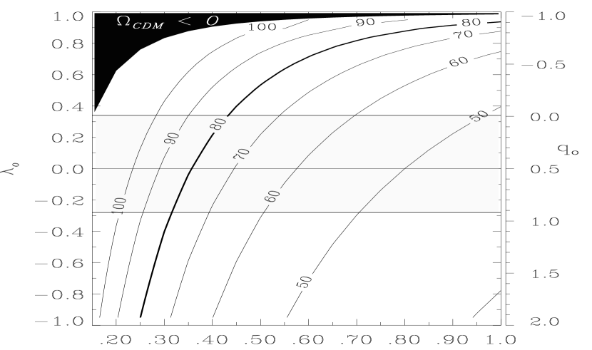
Fig. 6.: Contours of $A_{peak}\>[\mu$K] with $\Omega_{b}h^{2}=0.015$. As in Figure 3 no data were used to make this plot. The $80\>\mu$K contour is thick to indicate the approximate peak height of the data. For a given $h$, as $\lambda_{o}$ increases, $A_{peak}$ increases. The grey area marks the permitted area ($1\sigma$) from new supernovae results (Perlmutter et al.1997). All models in this plot have $\Omega_{o}+\lambda_{o}=1$.

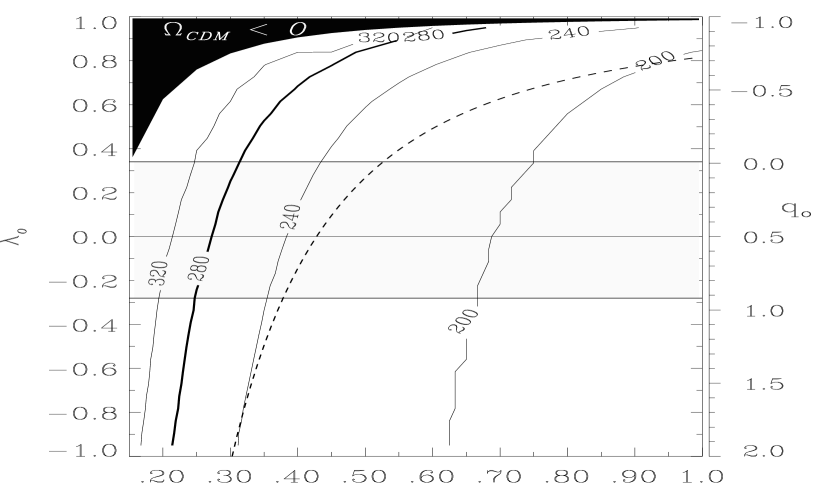
Fig. 7.: Contours of $\ell_{peak}$ for the same models as in Figure 6. Although no data were used to make this plot, the thick 280 contour is in the center of the region favored by the data. The dashed line is discussed in Section 3.2.2.

3.2.2 Peak Position

Hu & Sugiyama (1995b) identify three factors which, when increased, increase $\ell_{peak}$: $\Omega_{b}h^{2}$, $\lambda_{o}$ and $(1-\Omega_{o}-\lambda_{o})$. And one factor which, when increased, decreases $\ell_{peak}$, $\Omega_{o}h^{2}$. For all our models $1-\Omega_{o}-\lambda_{o}=0$, so this focusing effect plays no role here. The effect of $\Omega_{b}h^{2}$ can be understood using its relationship to the sound speed at recombination: $c_{s}=(1+a\Omega_{b}h^{2})^{-1/2}$ where $a$ is a constant, thus if $\Omega_{b}h^{2}\Uparrow$ $c_{s}\Downarrow$. The size of the fluctuations is controlled by the sound horizon at decoupling, thus $\theta_{peak}\propto c_{s}$. If $c_{s}\Downarrow$ then $\theta_{peak}\Downarrow$ and thus $\ell_{peak}\Uparrow$. We can see this clearly in the upper right of Figure 4. $\Omega_{b}h^{2}$ and $\Omega_{cdm}h^{2}$ have opposite effects on the peak amplitude and location. When $\Omega_{b}h^{2}\Uparrow\ell_{peak}\Uparrow$ and $A_{peak}\Uparrow$. When $\Omega_{cdm}h^{2}\Uparrow\ell_{peak}\Downarrow$ and $A_{peak}\Downarrow$.

The location of the peak plays an important role in preferring the low $h$ region of iso-$A_{peak}$ contours. The CMB data have $\ell_{peak}\sim 280$ which corresponds to an angular scale of $\sim 0^{\circ}\!.5$. In the lower right of Figures 4 and 7, $\ell_{peak}\sim 210$ (substantially lower than 280). Thus the data disfavor these high $h$ models.

There is an interesting apparent inconsistency in Figure 7. In the entire figure $\Omega_{b}h^{2}=0.015=constant$. Along the dashed line $\Omega_{o}h^{2}=\Omega_{b}h^{2}+\Omega_{cdm}h^{2}=0.015+(0.41)^{2}=constant$. Thus as we follow the dashed line up, $\lambda_{o}$ increases and we should see $\ell_{peak}$ increasing since, as we mentioned earlier if $\lambda_{o}\Uparrow$ then $\ell_{peak}\Uparrow$. This is not the case however; as we follow the dashed line upwards, $\ell_{peak}$ decreases. A scaling argument can clarify this. The angle $\theta$ subtended by an object of size $ct$ at an angular distance $d_{ang}$ is $\theta\sim ct/d_{ang}$. Thus,

$$\ell_{peak}\sim\frac{1}{\theta_{peak}}\sim\frac{d_{ang}(h,\Omega_{o},\lambda_{o})}{c\;t_{rec}}\sim\frac{h^{-1}f(\Omega_{o},\lambda_{o})}{(\Omega_{o}h^{2})^{-1/2}}\sim\frac{f(\lambda_{o})}{h}$$ (6)

where $\theta_{peak}$ is the angular scale of the Doppler peak. The physical scale of the peak oscillations is some fixed fraction of the horizon $\propto c\;t_{rec}$. The time of recombination scales as $(\Omega_{o}h^{2})^{-1/2}$ (which is constant along the dashed line) and the angular distance $d_{ang}=h^{-1}f(\Omega_{o},\lambda_{o})$. Since in our flat models $\Omega_{o}=1-\lambda_{o}$, $f(\Omega_{o},\lambda_{o})\rightarrow f(\lambda_{o})$ where

$$f(\lambda_{o})=\int_{0}^{z_{rec}}\frac{dz}{\left[(1+z)^{3}-\lambda_{o}(1+z)^{3}\right]^{1/2}}.$$ (7)

which, when inserted into equation (6) is an expression of the monotonic relation, when $\lambda_{o}\Uparrow$ then $\ell_{peak}\Uparrow$. However, for flat $\lambda_{o}$ models with $\Omega_{b}h^{2}$ and $\Omega_{cdm}h^{2}$ fixed, one cannot change $\lambda_{o}$ without changing $h$. So, in the case we are considering equation (6) is telling us that when $\frac{f(\lambda_{o})}{h}\Uparrow\ell_{peak}\Uparrow$. The $h$ scaling can be understood as the effect of larger universes: a given physical size at a larger distance subtends a smaller angle.

Following the pioneering work of Hu & Sugiyama (1995a, 1995b), in this section we have presented contours of the solutions of the Boltzmann equation and we have discussed how the behavior of $A_{peak}$ and $\ell_{peak}$ can be explained in terms of $\Omega_{b}h^{2}$ and $\Omega_{cdm}h^{2}$. These contour plots are particularly relevant for the next section where we describe the regions of solution space preferred by the CMB data.

4 $h-\Omega_{b}$ Results and Discussion

The CMB data can constrain any parameter that changes the power spectrum at a level comparable with the error bars on the data. Figure 8 displays the $\chi^{2}\>$contours for models in the $h-\Omega_{b}$ plane and contains one of the main results of this paper. CMB observations alone exclude at $>95\%$ CL, more than half of this parameter space. The solid and dotted contours in Figure 8 are goodness-of-fit contours labeled with the probabilities of finding a $\chi^{2}\>$less than the calculated value at that point. For example, in our case there are 21 degrees of freedom (24 data points - 2 fitted parameters - 1 COBE normalization). The probability of obtaining a $\chi^{2}\>$value less than 23.8 is 68.3 % assuming uncorrelated measurements and Gaussian errors. Thus we have labeled the $\chi^{2}=23.8$ contour ‘68’. The levels plotted are $\chi^{2}=[17.2,23.8,32.6]$ corresponding to 30%, 68% and 95% respectively.

The solid-line contours include our estimate of the $14\%$ absolute calibration uncertainty shared by the 5 Saskatoon points. The thick dotted (68%) and thin dotted (95%) contours do not include the Saskatoon calibration uncertainty. Thus the Saskatoon errors do not affect the 95% contour in the left and upper right, nor the left side of the 68% contour. The effect of the Saskatoon calibration uncertainties is discussed further in Section 4.1.

Any data sensitive only to the peak height will yield contours as seen in Figure 3. Figures 3 and 8 are similar so peak height is dominating the fit. If $A_{peak}$ were the only factor, then a region straddling the $A_{peak}\sim 80\;\mu$K contour would be equally preferred by the data. However the goodness-of-fit statistic prefers a region that does not follow exactly any iso-$A_{peak}$ contour. There is a preference for the low $h$ part of an iso-$A_{peak}$ region.

Lower $h$ is preferred because of the location of $\ell_{peak}$ in the data. One can see in Figure 2 that at smaller $h$ the position of the peak is more aligned with the dotted (data) line. This can also be seen in Figure 4 where the $\ell_{peak}$ values in the lower right are substantially less than the $\sim 280$ of the data. This $\ell_{peak}$ mismatch disfavors the high $h$ part of the preferred iso-$A_{peak}$ region.

Fig. 8.: Likelihood region and goodness-of-fit contours of $\chi^{2}$. The similarity of this figure and Figure 3 is a measure of the domination of the fits by $A_{peak}$. The solid and dotted lines are goodness-of-fit contours. The solid contours (30%, 68%, 95%) include our estimate of the Saskatoon calibration errors; the dotted contours (68%(thick), 95%(thin)) do not. The lower thin 95% dotted contour is obvious but the upper 95% dotted contour is identical to, and therefore hidden by, the solid 95% contour. The two dark grey areas are the $68\%$ likelihood regions for Sk$0$ (left) and Sk$-14$ (right)(see text). Small values of $h$ are preferred. The region preferred by big bang nucleosynthesis ($0.010<\Omega_{b}h^{2}<0.026$) is the light grey band. The small box and triangle at $\Omega_{b}\approx 0.05$ are the two model spectra plotted in Figure 1.

4.1 Saskatoon Calibration Error

The 5 Saskatoon (Sk) measurements (Netterfield et al.1997) apparently span the Doppler peak and play an important role in our fitting procedure. All 5 points share a 14% absolute calibration error as indicated by the small squares above and below their central values in Figure 1. There is no systematic way to handle systematic errors. Adding 14% errors in quadrature to the statistical errors is not appropriate because these errors are 100% correlated in the 5 Sk points. We have examined the effect of these correlated errors is several ways. We have made $\chi^{2}\>$surfaces from the CMB data:
$\bullet$ using the 5 Sk points as listed in Table 1 (“Sk$0$”)
$\bullet$ adding 14% to the 5 Sk points, i.e., using the high small squares in Figure 1 as the central values (“Sk$+14$”)
$\bullet$ subtracting 14% from the 5 Sk points, i.e., using the lower small squares in Figure 1 as the central values (“Sk$-14$”).
The minimum $\chi^{2}\>$for these three cases are respectively, 20, 33 and 13 corresponding to goodness-of-fit contours of 48%, 96% and 9%. Thus Sk$0$ gives a reasonable fit, Sk$+14$ gives a bad fit and Sk$-14$ gives a fit that is a bit too good.

We take a conservative approach in our treatment of these calibration errors. We create a new surface by adopting at each point in the plane the minimum of these three $\chi^{2}\>$surfaces (Sk$+14$, Sk$0$ and Sk$-14$). In Figure 8 we plot the iso-$\chi^{2}$ contours from this new surface. We will call this the “Sk$\pm 14$” case. For this new surface the Sk$-14$ $\chi^{2}\>$surface determines the contours in the lower right while the Sk$0$ $\chi^{2}\>$surface determines the contours to the left and upper right. This is easy to understand with Figure 3; Sk$0$ has a higher peak than Sk$-14$. Thus Sk$0$ prefers $A_{peak}\sim 80\mu$K and Sk$-14$ prefers $A_{peak}\sim 70\;\mu$K. The Sk$+14$ surface is effectively eliminated because of its poor goodness-of-fit.

The contours in Figure 8 are conservative in the sense that they encompass a larger region than the corresponding contours without including the Saskatoon calibration uncertainty. The dotted contours are the 68% and 95% goodness-of-fit levels from Sk$0$. The solid lines are the goodness-of-fit levels from our Sk$\pm 14\%$ method. Thus Figure 8 shows where and by how much the Saskatoon calibration uncertainty reduces the constraining ability of the CMB data.

It is interesting to note that the rest of the data thinks that the Saskatoon values are too high in the sense that the $\chi^{2}\>$surface from Sk$-14$ has a lower minimum than the Sk$0$ surface. This can be quantified; we can guess at the correct Sk calibration by using the non-Sk data and the models while treating the common calibration uncertainty of the Sk points as a free parameter, i.e., we let the calibration vary and assume that one of the models is correct. The lowest $\chi^{2}\>$is obtained if the Saskatoon points are reduced by 24%; the non-Sk data would like to see the Sk points all lowered by 24%. This preference is however shallow: $\chi^{2}_{min}(Sk-24\%)=11.4$ while $\chi^{2}_{min}(Sk-14\%)=12.7$ and $\chi^{2}_{min}(Sk-0\%)=19.9$.

The fact that the fit to Sk$-14$ is a bit too good can be interpreted as some combination of the following:
$\bullet$ just chance
$\bullet$ non-Sk data prefer a peak height lower than the Sk measurements
$\bullet$ the error bars of the non-Sk points are over-estimated
$\bullet$ detections of small significance do not get reported or are reported as upper limits which have not been included in the data set
$\bullet$ observers are finding what they are supposed to find.

Reasonable goodness-of-fit is a prerequisite for $\chi^{2}\>$minimum parameters that are meaningful. In addition to the goodness-of-fit contours presented thus far we have used the minima of the Sk$0$, Sk$-14$ and Sk$+14$ $\chi^{2}\>$surfaces to define the best fit parameters and to define confidence levels around these minima. This procedure is correct when the goodness-of-fit is within some plausible range, commonly [5%,95%], thus the Sk$+14$ minimum is of questionable value. To obtain likelihood intervals on parameter values at the minimum of a 2-D $\chi^{2}$ surface one takes $\chi^{2}_{min}+2.3$ as the 68% contour and $\chi^{2}_{min}+6.2$ as the 95% contour (e.g. Press et al.1992). In Figure 8, the two dark grey areas are the $68\%$ likelihood regions for Sk$0$ (left) and Sk$-14$ (right). The preferred $h$ value is low and the confidence levels are smaller than the corresponding goodness-of-fit contours.

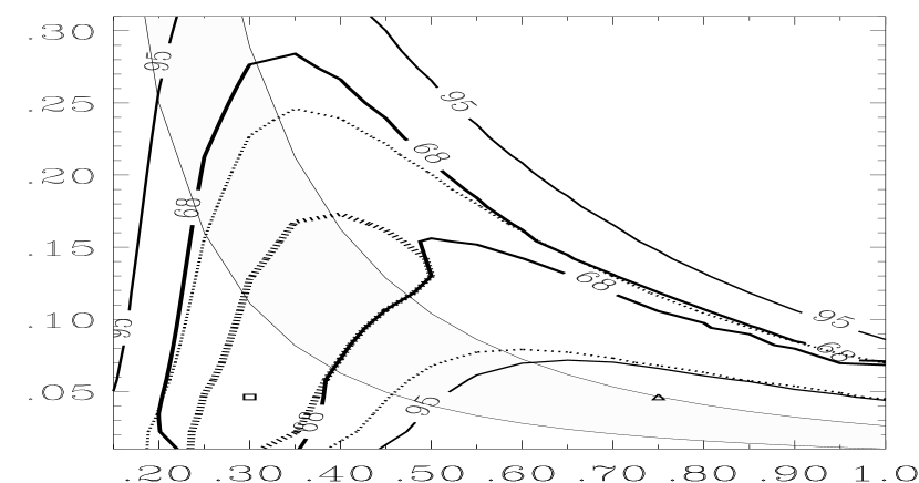
Fig. 9.: Same as Figure 8 except instead of the Saskatoon uncertainty, here we show the effect of the COBE normalization uncertainty. The dotted contours are the same as in Figure 8. The solid contours include our estimate of the effect of the COBE normalization uncertainty. They are the contours of a $\chi^{2}\>$surface constructed from the minima of three $\chi^{2}\>$surfaces, one each for $Q=16.4$, $18.0$ and $19.6$. The higher $Q$ value lets $\Omega_{b}$ be as high as 0.28. The limits on $h$ do not change substantially and thus small values of $h$ are still preferred independent of the COBE normalization uncertainty.

4.2 Normalization Uncertainty

So far we have assumed the COBE normalization $Q|_{n_{s}=1}=18\;\mu$K at $\ell=6$. However there is a $1.6\;\mu$K overall uncertainty on this value. To include this uncertainty in our results we make $\chi^{2}\>$contours for $Q=16.4$, $18.0$ and $19.6\;\mu$K. The minimum of the surfaces (produced by a procedure analogous to that used to make Figure 8) is shown in Figure 9 where the dotted contours do not, and the solid contours do, include the COBE normalization uncertainty. The normalization uncertainty increases the upper limit on $\Omega_{b}$ from 0.17 to 0.28 (68% CL). The limits on $h$ are robust to the normalization uncertainty. The lower right is still excluded.

4.3 Sensitivity to “Outliers”

One possible danger in using $\chi^{2}\>$goodness-of-fit contours is the influence of outliers. The overall level (goodness-of-fit) and possibly the shape of the contours around the minimum can be controlled by outliers. This depends on whether the models differ much at the $\ell_{eff}$ of the suspected outlier. For example in Figure 1, the COBE point at $\ell=25$ is an “outlier” which does nothing more than raise the entire $\chi^{2}\>$surface, since all models are the same at $\ell\sim 25$. This is not necessarily the case for the low MAX point (MAX HR) and certainly not for the 5 Saskatoon points. When the MAX HR point is excluded from the Sk$0$ surface calculation, the goodness-of-fit of the minimum improves from $\chi_{min}^{2}=20$ to $\chi^{2}_{min}=15$. The size and shape of the resulting contours do not change significantly, probably because at $\ell\approx 140$ the models are not substantially different.

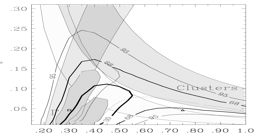
Fig. 10.: Same as Figure 8 except we have added two more constraints: Clusters: $0.04<\Omega_{b}h^{3/2}<0.10$ (White et al.1993) and the galaxy and cluster power spectrum shape parameter: $0.20<\Gamma<0.30$ (Peacock & Dodds 1994).

4.4 Result Summary

Our main results for the $h-\Omega_{b}$ plane are summarized in Figure 8. In the context of flat CDM universes, CMB observations can exclude more than half of the $h-\Omega_{b}$ parameter space explored. The CMB data favor low values of Hubble’s constant; $h\sim 0.35$. A higher value such as $h=0.75$ is permitted by the goodness-of-fit contours if $0.05<\Omega_{b}<0.09$ but these values are not within the 1-$\sigma$ likelihood region and are excluded by big bang nucleosynthesis (BBN). Low values of $\Omega_{b}$ are preferred ($\Omega_{b}\sim 0.03$) but the $\chi^{2}\>$minimum is shallow and we obtain $\Omega_{b}<0.28$ (68% CL).

These limits include our estimates for the Sk absolute calibration errors and the COBE normalization uncertainty. They are conservative in the sense that they are larger than the corresponding error bars around the parameters at the minimum of the $\chi^{2}\>$surfaces. Outliers do not seem to be biasing these results.

The CMB and BBN are independent observations. Thus, the overlapping of regions preferred by BBN and the CMB did not necessarily have to exist. The fact that they do is a consistency test for these two pillars of the big bang scenario.

The uncertainties in the BBN limits are dominated by systematic errors. Therefore we have used ‘weak’ BBN limits to try to avoid over-constraining the parameters. We have increased the limits of Copi et al.(1995), $0.010<\Omega_{b}h^{2}<0.020$, to include the higher values obtained by Tytler & Burles (1997), $0.022<\Omega_{b}h^{2}<0.026$. The credibility of the BBN constraints used here is important because their incompatibility with the CMB constraints at $h\mathrel{\mathchoice{\vbox{\offinterlineskip\halign{\hfil$\displaystyle#$\hfil\cr>\cr\sim\cr}}}{\vbox{\offinterlineskip\halign{\hfil$\textstyle#$\hfil\cr>\cr\sim\cr}}}{\vbox{\offinterlineskip\halign{\hfil$\scriptstyle#$\hfil\cr>\cr\sim\cr}}}{\vbox{\offinterlineskip\halign{\hfil$\scriptscriptstyle#$\hfil\cr>\cr\sim\cr}}}}70$ is what excludes these models. If one takes the maximum upper limit on $\Omega_{b}h^{2}$ as $0.045$ (Reeves 1994) then at the 68% CL all values of $h$ between $0.30$ and $1.0$ are permitted by even the combination of the CMB and BBN limits.

Figure 10 is the same as Figure 8 except we have added two more constraints: the White et al.(1993) limits from cluster baryon fractions: $0.04<\Omega_{b}h^{3/2}<0.10$, and the CDM shape parameter from a synthesis of the power spectra of galaxies and clusters: $0.20<\Gamma<0.30$ (Peacock & Dodds 1994). The similarity of the $\Gamma$ limits and the Sk$0$ contours is interesting. The inconsistency of BBN limits with the White et al.(1993) limits (assuming $\Omega_{o}=1$) is sometimes invoked as an argument for $\Omega_{o}<1$. However, as Figure 10 shows, this inconsistency disappears for the low $h$ values favored by the CMB data. An $\Omega_{o}=1$ model with $h\approx 0.40$, $\Omega_{b}\approx 0.15$ and $\Omega_{cdm}\approx 0.85$ is permitted by constraints from the CMB data, BBN, cluster baryon fractions and $\Gamma$.

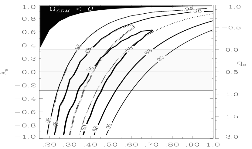
Fig. 11.: Goodness-of-fit contours of $\chi^{2}$ with $\Omega_{b}h^{2}=0.015$. As in Figure 8 the solid contours include the Saskatoon calibration uncertainty, the dotted do not. The grey area marks the permitted area (1 $\sigma$) from new supernovae results (Perlmutter et al.1997). For all models in this plot, $\Omega_{o}+\lambda_{o}=1$.

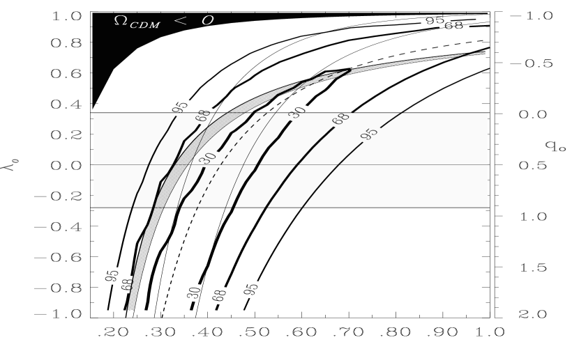
Fig. 12.: Same as Figure 11 except we have added two more constraints and left out the dotted contours for legibility. Constraints on the age of the universe ($13.7<t_{o}<17.9$) from the oldest stars (Bolte & Hogan 1995) are indicated by the thin solid lines. The dark grey area marks limits on the shape parameter: $0.20<\Gamma<0.30$ (Peacock & Dodds 1994). The thick dashed line through the minimum is $\Omega_{cdm}h^{2}=(0.41)^{2}$.

5 $h-\lambda_{o}$ Results and Discussion

In the previous section we described results in the $h-\Omega_{b}$ plane ($k=0$, $\Omega_{o}=1$, $\lambda_{o}=0$). In this section we present results for the $h-\lambda_{o}$ plane. ($k=0$, $\Omega_{o}+\lambda_{o}=1$). Figure 11 presents the $\chi^{2}\>$contours from fitting the data to these models. We are exploring a plane orthogonal to Figure 8. The same procedure used to make the contours in Figure 8 was used here. The notation is also the same; the solid contours include the Saskatoon calibration uncertainties, the dotted do not.

Figures 6 and 11 are similar for the same reason that Figures 3 and 8 are similar: $A_{peak}$ is the dominant feature of the fit. There is a slight preference for the low $h$ side of the preferred iso-$A_{peak}$ contour. Figure 7 helps explain this preference. For a given $\lambda_{o}$, $\ell_{peak}\sim 280$ is at a lower $h$ than the $A_{peak}\sim 80$ contour.

In this plane we obtain $0.23<h<0.72$ where these limits include our estimates for the uncertainties from the Saskatoon calibration, the COBE normalization and the BBN interval $0.010<\Omega_{b}h^{2}<0.026$. Assuming $\Omega_{b}h^{2}=0.015$, the CMB data yield $\lambda_{o}\mathrel{\mathchoice{\vbox{\offinterlineskip\halign{\hfil$\displaystyle#$\hfil\cr<\cr\sim\cr}}}{\vbox{\offinterlineskip\halign{\hfil$\textstyle#$\hfil\cr<\cr\sim\cr}}}{\vbox{\offinterlineskip\halign{\hfil$\scriptstyle#$\hfil\cr<\cr\sim\cr}}}{\vbox{\offinterlineskip\halign{\hfil$\scriptscriptstyle#$\hfil\cr<\cr\sim\cr}}}}0.9$ (68% CL) with lower values preferred. This is weaker than the traditional dynamical limit $\lambda_{o}\mathrel{\mathchoice{\vbox{\offinterlineskip\halign{\hfil$\displaystyle#$\hfil\cr<\cr\sim\cr}}}{\vbox{\offinterlineskip\halign{\hfil$\textstyle#$\hfil\cr<\cr\sim\cr}}}{\vbox{\offinterlineskip\halign{\hfil$\scriptstyle#$\hfil\cr<\cr\sim\cr}}}{\vbox{\offinterlineskip\halign{\hfil$\scriptscriptstyle#$\hfil\cr<\cr\sim\cr}}}}0.8$. A standard flat-$\lambda_{o}$ model is $\Omega_{o}\sim 0.3$ and $\lambda_{o}\sim 0.7$ with $h\approx.70$ This model is fully consistent with the CMB data. However the new SNIa results (Perlmutter et al.1997) rule it out; $-0.28\mathrel{\mathchoice{\vbox{\offinterlineskip\halign{\hfil$\displaystyle#$\hfil\cr<\cr\sim\cr}}}{\vbox{\offinterlineskip\halign{\hfil$\textstyle#$\hfil\cr<\cr\sim\cr}}}{\vbox{\offinterlineskip\halign{\hfil$\scriptstyle#$\hfil\cr<\cr\sim\cr}}}{\vbox{\offinterlineskip\halign{\hfil$\scriptscriptstyle#$\hfil\cr<\cr\sim\cr}}}}\lambda_{o}\mathrel{\mathchoice{\vbox{\offinterlineskip\halign{\hfil$\displaystyle#$\hfil\cr<\cr\sim\cr}}}{\vbox{\offinterlineskip\halign{\hfil$\textstyle#$\hfil\cr<\cr\sim\cr}}}{\vbox{\offinterlineskip\halign{\hfil$\scriptstyle#$\hfil\cr<\cr\sim\cr}}}{\vbox{\offinterlineskip\halign{\hfil$\scriptscriptstyle#$\hfil\cr<\cr\sim\cr}}}}0.34$ ($1\sigma$).

6 Summary and Discussion

We have explored solutions to the Boltzmann equation in two 2-D parameter spaces within the context of COBE normalized, Gaussian, adiabatic initial conditions in spatially flat universes with Harrison-Zel’dovich temperature fluctuations. We have presented the topology which controls the shapes of the acceptable regions for the cosmological parameters $h$, $\Omega_{b}$, and $\lambda_{o}$. We have fit a compilation of the most recent CMB measurements to the models and have identified regions favored and excluded by the data, i.e., we have fit the Boltzmann solutions to the CMB data and obtained constraints on the cosmological parameters $h$, $\Omega_{b}$, and $\lambda_{o}$.

Figures 8 and 11 contain the main results of this paper and are plots of the goodness-of-fit contours of the $\chi^{2}\>$from equation (1) using the data in Table 1. The solid contours mark the regions preferred by the data and include the Saskatoon calibration uncertainty. We obtain the following results:
$\bullet$ Recent CMB data are precise enough to prefer distinct regions of parameter space and rule out most of the $h-\Omega_{b}$ and $h-\lambda_{o}$ planes at the 95% CL.
$\bullet$ The CMB data favor low values of Hubble’s constant; $h\approx 0.35$. A higher value such as $h=0.75$ is permitted by the goodness-of-fit contours if $0.05<\Omega_{b}<0.09$ but these values are not within the 1-$\sigma$ likelihood region and are excluded by big bang nucleosynthesis (BBN).
$\bullet$ Low values of $\Omega_{b}$ are preferred ($\Omega_{b}\sim 0.03$) but the $\chi^{2}\>$minimum is shallow and we obtain $\Omega_{b}<0.28$.
$\bullet$ The CMB regions overlap with BBN. The fact that they do is a consistency test for these two pillars of the big bang scenario.
$\bullet$ A $\Omega_{o}=1$ model with $h\approx 0.40$, $\Omega_{b}\approx 0.15$ and $\Omega_{cdm}\approx 0.85$ is permitted by constraints from the CMB data, BBN, cluster baryon fractions and the shape parameter $\Gamma$ derived from the mass density power spectra of galaxies and clusters.
$\bullet$ For flat-$\lambda_{o}$ models, the CMB data, combined with BBN constraints exclude most of the $h-\lambda_{o}$ plane.
$\bullet$ Models with $\Omega_{o}\approx 0.3$, $\lambda_{o}\approx 0.7$ with $h\approx 0.75$ are fully consistent with the CMB data but are excluded by the strict new $q_{o}$ limits from supernovae.
$\bullet$ A combination of CMB data goodness-of-fit statistics, BBN and supernovae constraints in the $h-\lambda_{o}$ plane, limits Hubble’s constant to the interval $0.23<h<0.72$.

In this analysis we have made estimates of the errors associated with the Saskatoon absolute calibration uncertainty, the COBE normalization uncertainty, the uncertainty in BBN and we have considered the influence of possible outliers. We have assumed Gaussian adiabatic initial conditions. We have conditioned on the values $n_{s}=1$ and $Y_{He}=0.24$. We have ignored the possiblity of open universes, tilted spectra, early reionization and any gravity wave contribution to the spectra.

Our $h$ result is ‘low’ and inconsistent with several other recent $h$ measurements ($0.65\mathrel{\mathchoice{\vbox{\offinterlineskip\halign{\hfil$\displaystyle#$\hfil\cr<\cr\sim\cr}}}{\vbox{\offinterlineskip\halign{\hfil$\textstyle#$\hfil\cr<\cr\sim\cr}}}{\vbox{\offinterlineskip\halign{\hfil$\scriptstyle#$\hfil\cr<\cr\sim\cr}}}{\vbox{\offinterlineskip\halign{\hfil$\scriptscriptstyle#$\hfil\cr<\cr\sim\cr}}}}h\mathrel{\mathchoice{\vbox{\offinterlineskip\halign{\hfil$\displaystyle#$\hfil\cr<\cr\sim\cr}}}{\vbox{\offinterlineskip\halign{\hfil$\textstyle#$\hfil\cr<\cr\sim\cr}}}{\vbox{\offinterlineskip\halign{\hfil$\scriptstyle#$\hfil\cr<\cr\sim\cr}}}{\vbox{\offinterlineskip\halign{\hfil$\scriptscriptstyle#$\hfil\cr<\cr\sim\cr}}}}0.80$) in the sense that our 68% goodness-of-fit contours do not, but our 95% contours do include these higher $h$ values. The theoretical advantages of a low Hubble constant have been presented in Bartlett et al.(1995). For example, if $\Omega_{o}=1$ then a Hubble constant of $0.70$ implies an age of 9.3 Gyr, younger than the estimated ages of many globular clusters. However $h\sim 0.40$ yields an age of the universe of 16 Gyr, much more in accord with globular cluster ages.

If new data show that $A_{peak}\sim 70\;\mu$K rather than $80\;\mu$K and $\ell_{peak}\sim 230$ rather than 280, then the range $0.65\mathrel{\mathchoice{\vbox{\offinterlineskip\halign{\hfil$\displaystyle#$\hfil\cr<\cr\sim\cr}}}{\vbox{\offinterlineskip\halign{\hfil$\textstyle#$\hfil\cr<\cr\sim\cr}}}{\vbox{\offinterlineskip\halign{\hfil$\scriptstyle#$\hfil\cr<\cr\sim\cr}}}{\vbox{\offinterlineskip\halign{\hfil$\scriptscriptstyle#$\hfil\cr<\cr\sim\cr}}}}h\mathrel{\mathchoice{\vbox{\offinterlineskip\halign{\hfil$\displaystyle#$\hfil\cr<\cr\sim\cr}}}{\vbox{\offinterlineskip\halign{\hfil$\textstyle#$\hfil\cr<\cr\sim\cr}}}{\vbox{\offinterlineskip\halign{\hfil$\scriptstyle#$\hfil\cr<\cr\sim\cr}}}{\vbox{\offinterlineskip\halign{\hfil$\scriptscriptstyle#$\hfil\cr<\cr\sim\cr}}}}0.80$ may be acceptable to both the CMB and BBN constraints.

6.1 Acknowledgements

We gratefully acknowledge the use of the Boltzmann code kindly provided by Uros Seljak and Matias Zaldarriaga. We thank Martin White, Douglas Scott and the MAX group for help in assembling the required experimental window functions. We thank our referee, Douglas Scott, for comments that improved the clarity of this paper. We benefited from statistical discussions with Jean-Marie Hameury and Olivier Bienaymé. C.H.L. acknowledges support from the French Ministère des Affaires Etrangères. D.B. is supported by the Praxis XXI CIENCIA-BD/2790/93 grant attributed by JNICT, Portugal.

Table 1.: Data Used in the $\chi^{2}\>$Fit^a and Plotted in Figure 1

Experiment	reference	$\ell_{eff}$	$\delta T_{\ell_{eff}}^{data}\pm\sigma^{data}(\mu$K$)^{b}$
DMR1	[Hinshaw et al.(1996)]	3	$27.9_{-4.0}^{+5.6}$
DMR2	[Hinshaw et al.(1996)]	7	$24.6_{-2.8}^{+3.6}$
DMR3	[Hinshaw et al.(1996)]	14	$30.8_{-3.1}^{+3.4}$
DMR4	[Hinshaw et al.(1996)]	25	$1.2_{-1.2}^{+14.4}$
FIRS	[Ganga et al.(1994)]	10	$29.4_{-7.7}^{+7.8}$
Tenerife	[Hancock et al.(1996)]	19	$34.1_{-12.5}^{+12.5}$
SP91	[Gunderson et al.(1995)]	60	$30.2_{-5.5}^{+8.9}$
SP94	[Gunderson et al.(1995)]	60	$36.3_{-6.1}^{+13.6}$
Pyth1	[Platt et al.(1996)]	91	$54.0_{-12.0}^{+14.0}$
Pyth2	[Platt et al.(1996)]	176	$58.0_{-13.0}^{+15.0}$
ARGO1	[deBernardis et al.(1994)]	95	$39.1_{-8.7}^{+8.7}$
ARGO2	[Masi et al.(1996)]	95	$46.8_{-12.1}^{+9.5}$
MAX GUM	[Tanaka et al.(1996)]	138	$54.5_{-10.9}^{+16.4}$
MAX ID	[Tanaka et al.(1996)]	138	$46.3_{-13.6}^{+21.8}$
MAX SH	[Tanaka et al.(1996)]	138	$49.1_{-16.4}^{+21.8}$
MAX HR	[Tanaka et al.(1996)]	138	$32.7_{-8.2}^{+10.9}$
MAX PH	[Tanaka et al.(1996)]	138	$51.8_{-10.9}^{+19.1}$
Sk1	[Netterfield et al.(1997)]	86	$49.0_{-5.0}^{+8.0}$
Sk2	[Netterfield et al.(1997)]	166	$69.0_{-6.0}^{+7.0}$
Sk3	[Netterfield et al.(1997)]	236	$85.0_{-8.0}^{+10.0}$
Sk4	[Netterfield et al.(1997)]	285	$86.0_{-10.0}^{+12.0}$
Sk5	[Netterfield et al.(1997)]	348	$69.0_{-28.0}^{+19.0}$
CAT1	[Scott et al.(1996)]	396	$51.8_{-13.6}^{+13.6}$
CAT2	[Scott et al.(1996)]	607	$49.1_{-13.7}^{+19.1}$

^a CMB anisotropy detections reported in publications in 1994 and later. Many of the new result papers include reanalyses of older results. MSAM is not included because of substantial spatial and filter function overlap with Saskatoon.

${}^{b}\>$$Q_{flat}=Q_{rms-PS}|_{n_{s}=1}=(\frac{5}{12})^{1/2}\>\delta T_{\ell_{eff}}^{data}$.

References

- 1995 Bartlett, J., Blanchard, A., Silk, J., Turner, M.S. 1995, Science, 267, 980
- 1996 Bennett, C. L., et al.1996, Ap.J., 464, L1
- 1995 Bolte, M. & Hogan, C. 1995, Nature, 376, 399
- 1994 Bond, J.R., et al.1994, Phys. Rev. Lett., 72, 13
- 1995 Bond, J.R. 1995, Astrophys. Lett. and Comm., 32, 63
- 1995 Copi, C.J., Schram, D. N. & Turner, M.S. 1995, Science, 267, 192
- deBernardis et al.(1994) deBernardis, P., et al.1994, Ap.J., 422, L33
- Ganga et al.(1994) Ganga, K, Page, L., Cheng, E.S., Meyer, S. 1994, Ap.J., 432, L15
- 1996 Ganga, K, Ratra, B., and Sugiyama, N. 1996, Ap.J., 461, L61
- Gorski et al.(1994) Górski, K.,Ratra, B., Stompor, R., Sugiyama, N. and Banday, A.J. 1996, Ap.J., submitted, astro-ph/9608054
- Gunderson et al.(1995) Gunderson, J.O., et al.1995, Ap.J., 443, L57
- Hancock et al.(1996) Hancock, S. et al.1996, MNRAS, submitted
- Hinshaw et al.(1996) Hinshaw, G. et al.1996, Ap.J., 464, L17
- 1995 Hu W. 1995, Ph.D thesis, Berkeley
- 1995 Hu W. & Sugiyama, N. 1995a, Phys. Rev. D., 51, 2599
- 1995 Hu W. & Sugiyama, N. 1995b, Ap.J., 444, 489
- 1996 Jungmann, G., et al.1996, Phys. Rev. D., 54, 1332
- Masi et al.(1996) Masi, S. et al.1996, Ap.J., 463, L47
- Netterfield et al.(1997) Netterfield, C.B., et al.1997, Ap.J., 474, 47
- 1994 Peacock, J.A. & Dodds, S.J. 1994, MNRAS, 267, 1020
- 1997 Perlmutter, S. et al.1997, Ap.J., in press, astro-ph/9608192
- Platt et al.(1996) Platt, S.R. et al.1996, astro-ph/9606175
- 1995 Press, W., Teukolsky, S., Vettering, W. & Flannery, B. 1992, ‘Numerical Recipes (in Fortran)’, 2nd edition, Camb.Univ. Press (p 692)
- 1995 Ratra, B., Banday, A.J., Górski, K., Sugiyama, N. 1995, astro-ph/9512148
- 1994 Reeves, H. 1994, Rev. Mod. Phys., 66, 193
- 1996 Scott, D., et al.1995, Science, 268, 5212, 829
- Scott et al.(1996) Scott, P.F.S. et al.1996, Ap.J., 461, L1
- 1996 Seljak, U. & Zaldarriaga, M. 1996, Ap.J., 469, 437
- 1992 Smoot, G.F. et al.1992, Ap.J., 396, L1
- Tanaka et al.(1996) Tanaka, S., et al.1996, Ap.J., 468, L81
- 1997 Tytler, D. & Burles, S. in ‘Origin of Matter and Evolution of Galaxies in the Universe 1996’, edt. T. Kajino, Y. Yoshii, S. Kubono (World Scientific: Singapore), in press, 1997
- 1995 White, M. & Srednicki, M. 1995, Ap.J., 443, 6
- 1996 White, M., Viana, P.T.P., Liddle, A.R., Scott, D. 1996, MNRAS, 283, 107
- 1993 White, S.D.M., et al.1993, Nature, 366, 429